
Can Ensemble Machine Learning Methods Predict Stock Returns for Indian Banks Using Technical Indicators?

 ,
,
Abstract
1. Introduction
2. Literature Review
3. Data Description
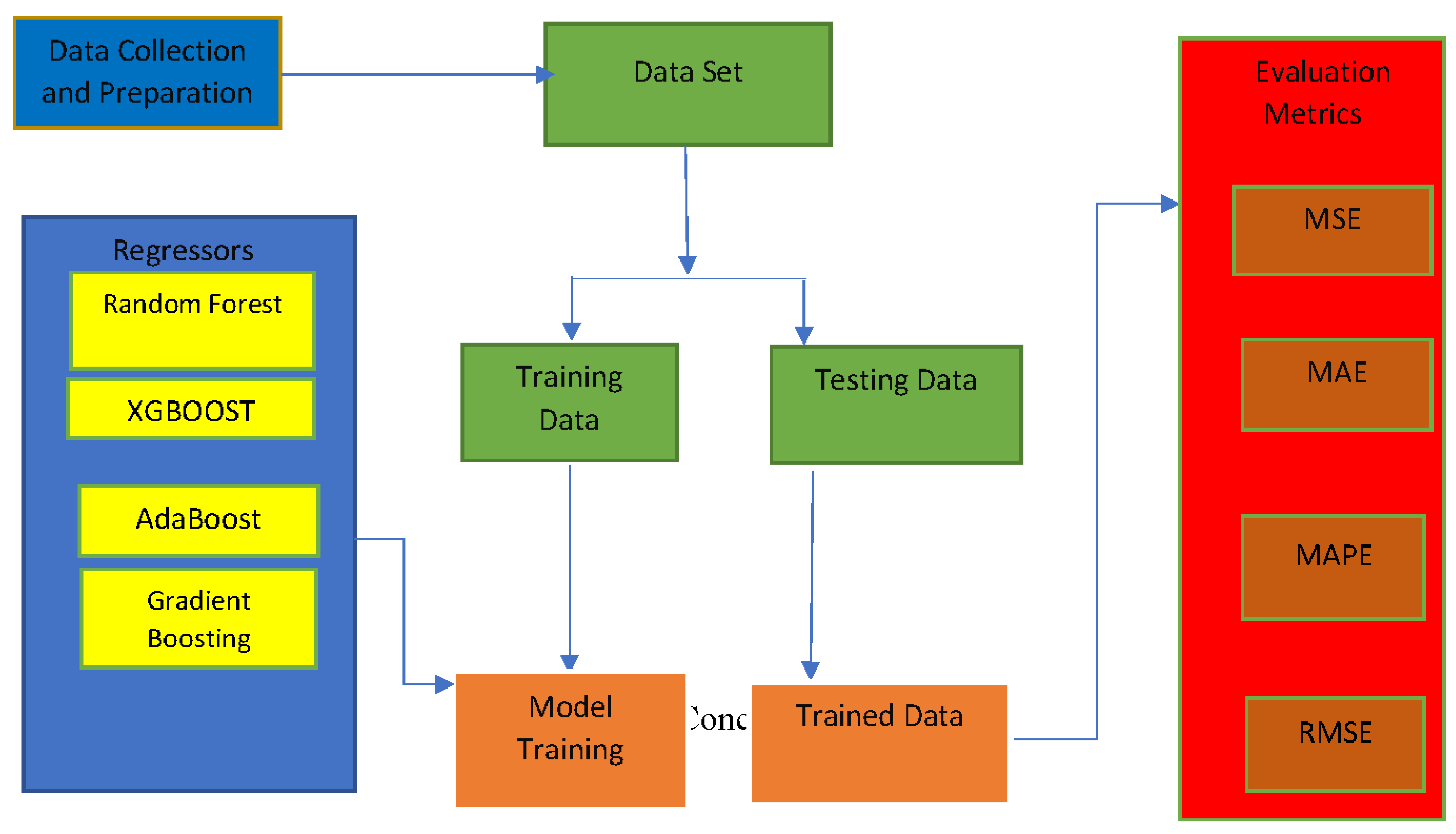
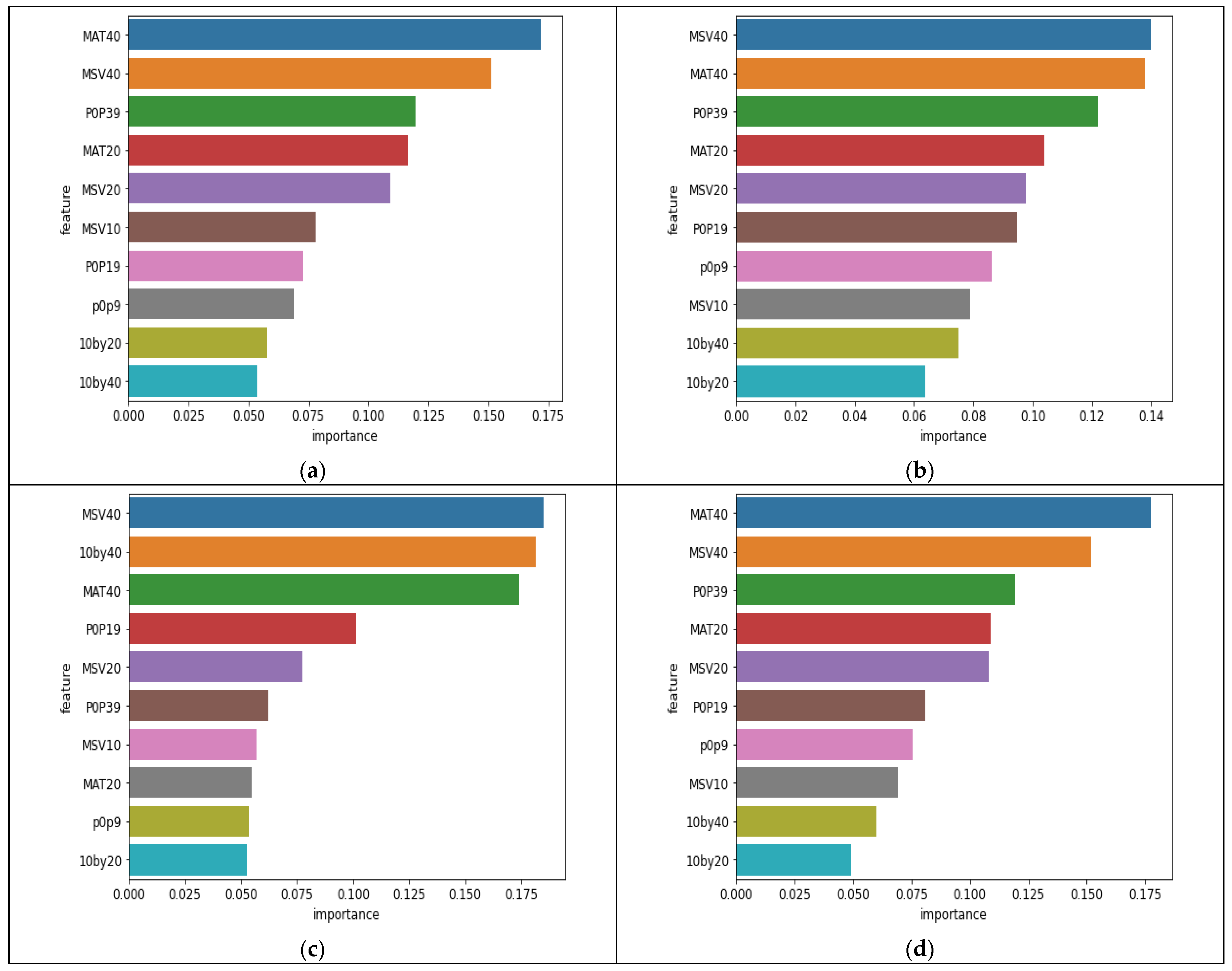
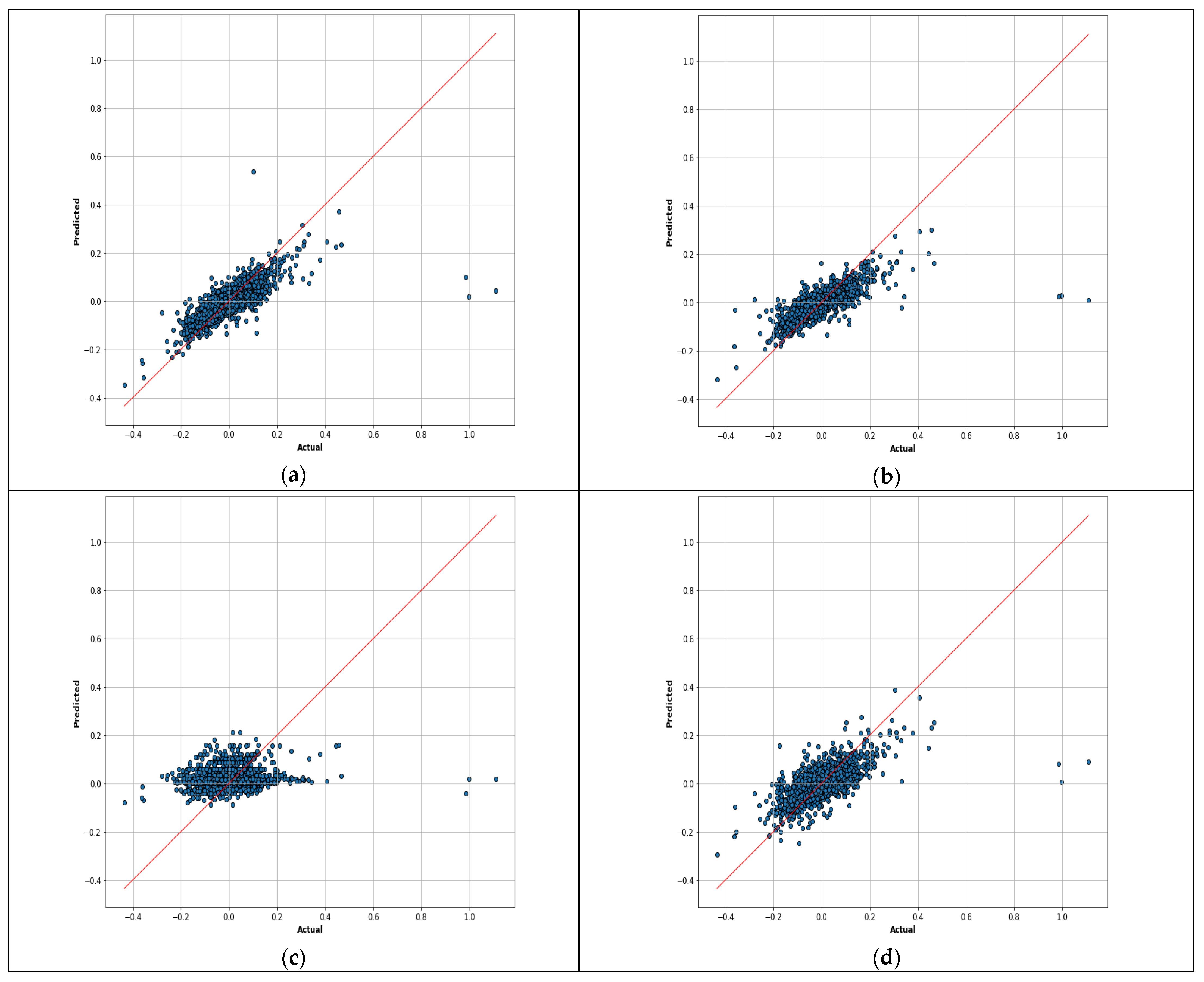
4. Methodology
4.1. Random Forest
4.2. AdaBoost
4.3. Gradient Boosting
4.4. XGBoost
4.5. Evaluating Metrics
5. Results
6. Conclusions
Author Contributions
Funding
Institutional Review Board Statement
Informed Consent Statement
Data Availability Statement
Conflicts of Interest
References
- Ajmi, Ahdi Noomen, Shawkat Hammoudeh, Duc Khuong Nguyen, and Soodabeh Sarafrazi. 2014. How strong are the causal relationships between Islamic stock markets and conventional financial systems? Evidence from linear and nonlinear tests. Journal of International Financial Markets, Institutions and Money 28: 213–27. [Google Scholar] [CrossRef]
- Alberg, John, and Zachary C. Lipton. 2017. Improving Factor-Based Quantitative Investing by Forecasting Company Fundamentals, (Nips). arXiv arXiv:1711.04837. [Google Scholar]
- Ampomah, Ernest Kwame, Zhiguang Qin, and Gabriel Nyame. 2020. Evaluation of Tree-Based Ensemble Machine Learning Models in Predicting Stock Price Direction of Movement. Information 11: 332. [Google Scholar] [CrossRef]
- Chatterjee, Ananda, Hrisav Bhowmick, and Jaydip Sen. 2021. Stock Price Prediction Using Time Series, Econometric, Machine Learning, and Deep Learning Models. Paper presented at 2021 IEEE Mysore Sub Section International Conference (MysuruCon), Hassan, India, October 24–25. [Google Scholar]
- Andriyashin, Anton, Wolfgang K. Härdle, and Roman Vladimirovich Timofeev. 2008. Recursive Portfolio Selection with Decision Trees. SFB 649 Discussion Paper 2008-009. Available online: https://ssrn.com/abstract=2894287 (accessed on 15 January 2008). [CrossRef][Green Version]
- Ayala, Jordan, Miguel García-Torres, José Luis Vázquez Noguera, Francisco Gómez-Vela, and Federico Divina. 2021. Technical analysis strategy optimization using a machine learning approach in stock market indices. Knowledge-Based Systems 225: 107119. [Google Scholar] [CrossRef]
- Belciug, Smaranda, and Adrian Victor Sandita. 2017. Business Intelligence: Statistics in predicting stock market. University of Craiova—Mathematics and Computer Science Series 44: 292–98. [Google Scholar]
- Breiman, Leo. 2001. Random forests. Machine Learning 45: 5–32. [Google Scholar] [CrossRef]
- Bustos, Oscar, and Alexandra Pomares-Quimbaya. 2020. Stock market movement forecast: A Systematic review. Expert Systems with Applications 156: 113464. [Google Scholar] [CrossRef]
- Carlini, Federico, Doriana Cucinelli, Daniele Previtali, and Maria Gaia Soana. 2020. Don’t talk too bad! stock market reactions to bank corporate governance news. Journal of Banking & Finance 121: 105962. [Google Scholar]
- Challa, Madhavi Latha, Venkataramanaiah Malepati, and Siva Nageswara Rao Kolusu. 2020. S&p bse sensex and s&p bse it return forecasting using arima. Financial Innovation 6: 47. [Google Scholar]
- Chang, Tsung-Sheng. 2011. A comparative study of artificial neural networks, and decision trees for digital game content stocks price prediction. Expert Systems with Applications 38: 14846–51. [Google Scholar] [CrossRef]
- Chen, Tianqi, and Carlos Guestrin. 2016. XGBoost: A Scalable Tree Boosting System. Paper presented at KDD ’16: The 22nd ACM SIGKDD International Conference on Knowledge Discovery and Data Mining, San Francisco, CA, USA, August 13–17; pp. 785–94. [Google Scholar] [CrossRef]
- Chen, Yufeng, Jinwang Wu, and Zhongrui Wu. 2022. China’s commercial bank stock price prediction using a novel K-means-LSTM hybrid approach. Expert Systems with Applications 202: 117370. [Google Scholar] [CrossRef]
- Cheng, Xu, Winston Wei Dou, and Zhipeng Liao. 2022. Macro-Finance Decoupling: Robust Evaluations of Macro Asset Pricing Models. Econometrica 90: 685–713. [Google Scholar] [CrossRef]
- Chong, Eunsuk, Chulwoo Han, and Frank C. Park. 2017. Deep learning networks for stock market analysis and prediction: Methodology, data representations, and case studies. Expert Systems with Applications 83: 187–205. [Google Scholar] [CrossRef]
- Chou, Jui-Shwng, and Thi-Kha Nguyen. 2018. Forward forecast of stock price using sliding-window metaheuristic-optimized machine-learning regression. IEEE Transactions on Industrial Informatics 14: 3132–42. [Google Scholar] [CrossRef]
- Choudhry, Rohit, and Kumkum Garg. 2008. A hybrid machine learning system for stock market forecasting. World Academy of Science, Engineering and Technology 39: 315–18. [Google Scholar]
- Ciner, Cetin. 2019. Do industry returns predict the stock market? A reprise using the random forest. The Quarterly Review of Economics and Finance 72: 152–58. [Google Scholar] [CrossRef]
- Coyne, Scott, Praveen Madiraju, and Joseph Coelho. 2018. Forecasting stock prices using social media analysis. Paper presented at 2017 IEEE 15th International Conference on Dependable, Autonomic and Secure Computing, 15th International Conference on Pervasive Intelligence and Computing, 3rd International Conference on Big Data Intelligence and Computing and Cyber Science and Technology Congress (DASC/PiCom/DataCom/CyberSciTech), Orlando, FL, USA, November 6–10. [Google Scholar]
- Dai, Zhifeng, Xiaodi Dong, Jie Kang, and Lianying Hong. 2020. Forecasting stock market returns: New technical indicators and two-step economic constraint method. The North American Journal of Economics and Finance 53: 101216. [Google Scholar] [CrossRef]
- Day, Min-Yuh, Yensen Ni, Chinning Hsu, and Paoyu Huang. 2022. Do Investment Strategies Matter for Trading Global Clean Energy and Global Energy ETFs? Energies 15: 3328. [Google Scholar] [CrossRef]
- De Oliveira, Fagner A., Cristiane N. Nobre, and Luis E. Zárate. 2013. Applying Artificial Neural Networks to prediction of stock price and improvement of the directional prediction index–Case study of PETR4, Petrobras, Brazil. Expert Systems with Applications 40: 7596–606. [Google Scholar] [CrossRef]
- Dutta, Goutam, Pankaj Jha, Arnab Kumar Laha, and Neeraj Mohan. 2006. Artificial neural network models for forecasting stock price index in the Bombay stock exchange. Journal of Emerging Market Finance 5: 283–95. [Google Scholar] [CrossRef]
- Edmans, Alex, Itay Goldstein, and Wei Jiang. 2012. Feedback Effects and the Limits to Arbitrage. Working Paper 17582. Cambridge: National Bureau of Economic Research. [Google Scholar]
- Fama, Eugene F. 1970. Efficient capital markets: A review of theory and empirical work. The Journal of Finance 25: 383–417. [Google Scholar] [CrossRef]
- Fama, Eugene F., and Kenneth R. French. 1993. Common risk factors in the returns on stocks and bonds. Journal of Financial Economics 33: 3–56. [Google Scholar] [CrossRef]
- Fama, Eugene F., and Kenneth R. French. 2015. A five-factor asset pricing model. Journal of Financial Economics 116: 1–22. [Google Scholar] [CrossRef]
- Freund, Yoav, Robert E. Schapire, and Naoki Abe. 1999. A short introduction to boosting. Journal-Japanese Society for Artificial Intelligence 14: 1612. [Google Scholar]
- Friedman, Jerome H. 2002. Stochastic gradient boosting. Computational Statistics & Data Analysis 38: 367–78. [Google Scholar]
- Guiso, Luigi, Paola Sapienza, and Luigi Zingales. 2008. Trusting the stock market. Journal of Finance 63: 2557–600. [Google Scholar] [CrossRef]
- Guiso, Luigi, Paola Sapienza, and Luigi Zingales. 2011. Time Varying Risk Aversion. Working Paper. Evanston: Northwestern University. [Google Scholar]
- Guresen, Erkam, Gulgun Kayakutlu, and Tugrul U. Daim. 2011. Using artificial neural network models in stock market index prediction. Expert Systems with Applications 38: 10389–97. [Google Scholar] [CrossRef]
- Hanauer, Matthias X., Marina Kononova, and Marc Steffen Rapp. 2022. Boosting Agnostic Fundamental Analysis: Using Machine Learning to Identify Mispricing in European Stock Markets. Finance Research Letters 48: 102856. [Google Scholar] [CrossRef]
- Hellström, Thomas, and Kenneth Holmström. 1998. Predictable Patterns in Stock Returns. Published as Opuscula ISRN HEV-BIB-OP-30-SE. Västerås: Center of Mathematical Modeling, Department of Mathematics and Physics, Mälardalen University. 31p. [Google Scholar]
- Hsu, Ming-Wei, Stefan Lessmann, Ming-Chien Sung, Tiejun Ma, and Johnnie E. V. Johnson. 2016. Bridging the divide in financial market forecasting: Machine learners vs. financial economists. Expert Systems with Applications 61: 215–34. [Google Scholar] [CrossRef]
- Hu, Hongping, Li Tang, Shuhua Zhang, and Haiyan Wang. 2018. Predicting the direction of stock markets using optimized neural networks with Google Trends. Neurocomputing 285: 188–95. [Google Scholar] [CrossRef]
- Huang, Chin-Sheng, and Yi-Sheng Liu. 2019. Machine learning on stock price movement forecast: The sample of the Taiwan stock exchange. International Journal of Economics and Financial Issues 9: 189. [Google Scholar]
- Kara, Yakup, Melek Acar Boyacioglu, and Ömer Kaan Baykan. 2011. Predicting direction of stock price index movement using artificial neural networks and support vector machines: The sample of the Istanbul Stock Exchange. Expert Systems with Applications 38: 5311–19. [Google Scholar] [CrossRef]
- Kazem Ahad, Ebrahim Sharifi, Farookh Khadeer Hussain, Morteza Saberi, and Omar Khadeer Hussain. 2013. Support vector regression with chaos-based firefly algorithm for stock market price forecasting. Applied Soft Computing 13: 947–58. [Google Scholar] [CrossRef]
- Khashei, Mehdi, and Mehdi Bijari. 2010. An artificial neural network (p, d, q) model for timeseries forecasting. Expert Systems with Applications 37: 479–89. [Google Scholar] [CrossRef]
- Kim, Kyoung-jae, and Ingoo Han. 2000. Genetic algorithms approach to feature discretization in artificial neural networks for the prediction of stock price index. Expert Systems with Applications 19: 125–32. [Google Scholar] [CrossRef]
- Kim, Sondo, Seungmo Ku, Woojin Chang, and Jae Wook Song. 2020. Predicting the direction of US stock prices using effective transfer entropy and machine learning techniques. IEEE Access 8: 111660–82. [Google Scholar] [CrossRef]
- Kolarik, Thomas, and Gottfried Rudorfer. 1994. Time series forecasting using neural networks. ACM Sigapl Apl Quote Quad 25: 86–94. [Google Scholar] [CrossRef]
- Krauss, Christopher, Xuan Anh Do, and Nicolas Huck. 2017. Deep neural networks, gradient-boosted trees, random forests: Statistical arbitrage on the S&P 500. European Journal of Operational Research 259: 689–702. [Google Scholar]
- Kraus, Mathias, and Stefan Feuerriegel. 2017. Decision support from financial disclosures with deep neural networks and transfer learning. Decision Support Systems 104: 38–48. [Google Scholar] [CrossRef]
- Kristjanpoller, Werner, and Kevin Michell. 2018. A stock market risk forecasting model through integration of switching regime, ANFIS and GARCH techniques. Applied Soft Computing 67: 106–16. [Google Scholar] [CrossRef]
- Kumar, Manish, and M. Thenmozhi. 2007. Support vector machines approach to predict the S&P CNX NIFTY index returns. In 10th Capital Markets Conference, Indian Institute of Capital Markets Paper. Maharashtra: Indian Institute of Capital Markets. [Google Scholar]
- Lei, Lei. 2018. Wavelet neural network prediction method of stock price trend based on rough set attribute reduction. Applied Soft Computing 62: 923–32. [Google Scholar] [CrossRef]
- Leung, Edward, Harald Lohre, David Mischlich, Yifei Shea, and Maximilian Stroh. 2021. The promises and pitfalls of machine learning for predicting stock returns. The Journal of Financial Data Science 3: 21–50. [Google Scholar] [CrossRef]
- Majhi, Ritanjali, Ganapati Panda, and Gadadhar Sahoo. 2009. Development and performance evaluation of FLANN based model for forecasting of stock markets. Expert Systems with Applications 36: 6800–8. [Google Scholar] [CrossRef]
- Meesad, Phayung, and Risul Islam Rasel. 2013. Predicting stock market price using support vector regression. Paper present at 2013 International Conference on Informatics, Electronics and Vision (ICIEV), Dhaka, Bangladesh, May 17–18; pp. 1–6. [Google Scholar]
- Naik, Nagaraj, and Biju R. Mohan. 2020. Intraday stock prediction based on deep neural network. National Academy Science Letters 43: 241–46. [Google Scholar] [CrossRef]
- Neely, Christopher J., David E. Rapach, Jun Tu, and Guofu Zhou. 2014. Forecasting the equity risk premium: The role of technical indicators. Management Science 60: 1772–91. [Google Scholar] [CrossRef]
- Nti, Isaac Kofi, Adebayo Felix Adekoya, and Benjamin Asubam Weyori. 2020. A comprehensive evaluation of ensemble learning for stock-market prediction. Journal of Big Data 7: 20. [Google Scholar] [CrossRef]
- Panda, Chakradhara, and V. Narasimhan. 2007. Forecasting exchange rate better with artificial neural network. Journal of Policy Modeling 29: 227–36. [Google Scholar] [CrossRef]
- Park, Hyun Jun, Youngjun Kim, and Ha Young Kim. 2022. Stock market forecasting using a multi-task approach integrating long short-term memory and the random forest framework. Applied Soft Computing 114: 108106. [Google Scholar] [CrossRef]
- Patel, Jigar, Sahil Shah, Priyank Thakkar, and K. Kotecha. 2015. Predicting stock and stock price index movement using trend deterministic data preparation and machine learning techniques. Expert Systems with Applications 42: 259–68. [Google Scholar] [CrossRef]
- Qiu, Mingyue, and Yu Song. 2016. Predicting the direction of stock market index movement using an optimized artificial neural network model. PLoS ONE 11: e0155133. [Google Scholar] [CrossRef]
- Qiu, Mingyue, Cheng Li, and Yu Song. 2016. Application of the Artificial Neural Network in predicting the direction of stock market index. Paper presented at 2016 10th International Conference on Complex, Intelligent, and Software Intensive Systems (CISIS), Fukuoka, Japan, July 6–8; pp. 219–23. [Google Scholar]
- Rahman, Molla Ramizur, and Arun Kumar Misra. 2021. Bank Competition Using Networks: A Study on an Emerging Economy. Journal of Risk and Financial Management 14: 402. [Google Scholar] [CrossRef]
- Rasekhschaffe, Keywan, and Robert Jones. 2019. Machine learning for stock selection. Financial Analysts Journal 75: 70–88. [Google Scholar] [CrossRef]
- Sadorsky, Perry. 2021. A random forests approach to predicting clean energy stock prices. Journal of Risk and Financial Management 14: 48. [Google Scholar] [CrossRef]
- Shen, Shunrong, Haomiao Jiang, and Tongda Zhang. 2012. Stock Market Forecasting Using Machine Learning Algorithms. Stanford: Department of Electrical Engineering, Stanford University, pp. 1–5. [Google Scholar]
- Shetty, Shekar, Mohamed Musa, and Xavier Brédart. 2022. Bankruptcy Prediction Using Machine Learning Techniques. Journal of Risk and Financial Management 15: 35. [Google Scholar] [CrossRef]
- Song, Yue-Gang, Yu-Long Zhou, and Ren-Jie Han. 2018. Neural networks for stock price prediction. arXiv arXiv:1805.11317. [Google Scholar]
- Sorensen, Eric H., Keith L. Miller, and Chee K. Ooi. 2000. The decision tree approach to stock selection. The Journal of Portfolio Management 27: 42–52. [Google Scholar] [CrossRef]
- Tsibouris, George, and Matthew Zeidenberg. 1995. Testing the efficient markets hypothesis with gradient descent algorithms. In Neural Networks in the Capital Markets. Hoboken: John Wiley & Sons. [Google Scholar]
- Wang, Sheng, Yin Luo, Rochester Cahan, Miguel A. Alvarez, Javed Jussa, and Zongye Chen. 2012. Signal processing: The rise of the machines. Deutsche Bank Quantitative Strategy, June 5. [Google Scholar]
- White, Halbert. 1988. Economic prediction using neural networks: The case of IBM daily stock returns. Paper presented at International Conference on Neural Networks (ICNN ’88), San Diego, CA, USA, July 24–27, vol. 2, pp. 451–58. [Google Scholar]
- Wu, Jimmy Ming-Tai, Zhongcui Li, Gautam Srivastava, Meng-Hsiun Tasi, and Jerry Chun-Wei Lin. 2021. A graph-based convolutional neural network stock price prediction with leading indicators. Software: Practice and Experience 51: 628–44. [Google Scholar] [CrossRef]
- Zhang, Yuchen, and Shigeyuki Hamori. 2020. The predictability of the exchange rate when combining machine learning and fundamental models. Journal of Risk and Financial Management 13: 48. [Google Scholar] [CrossRef]
- Zhao, Yang, Jianping Li, and Lean Yu. 2017. A deep learning ensemble approach for crude oil price forecasting. Energy Economics 66: 9–16. [Google Scholar] [CrossRef]
- Zhang, Jin-Liang, Yue-Jun Zhang, and Lu Zhang. 2015. A novel hybrid method for crude oil price forecasting. Energy Economics 49: 649–59. [Google Scholar] [CrossRef]
- Zhong, Xiao, and David Enke. 2017. A comprehensive cluster and classification mining procedure for daily stock market return forecasting. Neurocomputing 267: 152–68. [Google Scholar] [CrossRef]
- Zhu, Min, David Philpotts, and Maxwell J. Stevenson. 2012. The benefits of tree-based models for stock selection. Journal of Asset Management 13: 437–48. [Google Scholar] [CrossRef]
- Zhu, Min, David Philpotts, Ross Sparks, and Maxwell J. Stevenson. 2011. A hybrid approach to combining CART and logistic regression for stock ranking. Journal of Portfolio Management 38: 100–9. [Google Scholar] [CrossRef]


| Factors | Description | Mathematical Computation |
|---|---|---|
| 10by20 10by40 |
| where, m1 ϵ (10), m2 ϵ (20, 40) |
| MAT20 MAT40 |
| movavg (turn over, m) where, m ϵ (20, 40) |
| MSV10 MSV20 MSV40 |
| movstd (volume, m) where, m ϵ (10, 20, 40) |
| P0P9 P0P19 P0P39 |
| ; where, m ϵ (9, 19, 39) |
| Random Forest | XGBOOST | AdaBoost | Gradient Boosting | |
|---|---|---|---|---|
| MSE | 0.0034 | 0.0030 | 0.0081 | 0.0041 |
| MAE | 0.0353 | 0.0327 | 0.0647 | 0.0423 |
| MAPE | 1.5644 | 1.7451 | 3.3125 | 2.2779 |
| RMSE | 0.0588 | 0.0550 | 0.0904 | 0.0645 |
Publisher’s Note: MDPI stays neutral with regard to jurisdictional claims in published maps and institutional affiliations. |
© 2022 by the authors. Licensee MDPI, Basel, Switzerland. This article is an open access article distributed under the terms and conditions of the Creative Commons Attribution (CC BY) license (https://creativecommons.org/licenses/by/4.0/).
Share and Cite
Mohapatra, S.; Mukherjee, R.; Roy, A.; Sengupta, A.; Puniyani, A. Can Ensemble Machine Learning Methods Predict Stock Returns for Indian Banks Using Technical Indicators? J. Risk Financial Manag. 2022, 15, 350. https://doi.org/10.3390/jrfm15080350
Mohapatra S, Mukherjee R, Roy A, Sengupta A, Puniyani A. Can Ensemble Machine Learning Methods Predict Stock Returns for Indian Banks Using Technical Indicators? Journal of Risk and Financial Management. 2022; 15(8):350. https://doi.org/10.3390/jrfm15080350
Chicago/Turabian StyleMohapatra, Sabyasachi, Rohan Mukherjee, Arindam Roy, Anirban Sengupta, and Amit Puniyani. 2022. "Can Ensemble Machine Learning Methods Predict Stock Returns for Indian Banks Using Technical Indicators?" Journal of Risk and Financial Management 15, no. 8: 350. https://doi.org/10.3390/jrfm15080350
APA StyleMohapatra, S., Mukherjee, R., Roy, A., Sengupta, A., & Puniyani, A. (2022). Can Ensemble Machine Learning Methods Predict Stock Returns for Indian Banks Using Technical Indicators? Journal of Risk and Financial Management, 15(8), 350. https://doi.org/10.3390/jrfm15080350