Model Selection and Post Selection to Improve the Estimation of the ARCH Model

Abstract

The Autoregressive Conditionally Heteroscedastic (ARCH) model is useful for handling volatilities in economical time series phenomena that ARIMA models are unable to handle. The ARCH model has been adopted in many applications that contain time series data such as financial market prices, options, commodity prices and the oil industry. In this paper, we propose an improved post-selection estimation strategy. We investigated and developed some asymptotic properties of the suggested strategies and compared with a benchmark estimator. Furthermore, we conducted a Monte Carlo simulation study to reappraise the relative characteristics of the listed estimators. Our numerical results corroborate with the analytical work of the study. We applied the proposed methods on the S&P500 stock market daily closing prices index to illustrate the usefulness of the developed methodologies.

1. Introduction

Modeling and forecasting financial markets are a challenging activities for both investors and researchers equally. Generally, financial markets are extremely manipulated by a number of factors such as interest rates, political issues, inflation rates and foreign exchange rates. More precisely, the uncertainty of stock markets produces high volatility that makes the forecasting stage very complex. Volatility forecasting is an important financial matter, and a precise and accurate volatility forecast is important to traders, investors and financial analysts. Before the 1980s, researchers were relying on ARIMA models, however, many financial time series violate the assumptions of the ARIMA model (cf. Brockwell and Davis 2016; Teräsvirta 2009).

Fortunately, Engle (1982) suggested a stationary non-linear model for economical time series and introduced the Autoregressive Conditionally Heteroscedastic (ARCH) model, wherein the conditional variance of a series $\left\{y_k\right\}$ changes according to an autoregressive-type process. Subsequently, Francq and Zakoïan (2012); Grublytė et al. (2017) discussed the properties of maximum likelihood (MLE) and ordinary least squares (OLS) estimates of ARCH model parameters. They also investigated the consistency and the asymptotic normality of the OLS estimator for the ARCH model.

In this article, we are interested in estimating the parameter vector of the ARCH model when some prior information is available in the form of potential linear restrictions on the parameters in the parameter space. Practically, an ample number of variables may be collected and included in the model in an initial stage. However, due to model complexity (in terms of both interpretation and variation), estimation when a subset of parameters are under linear restrictions is an important problem in such scenarios. In order to form such constraints, one requires some prior information about the parameter space under consideration. One possible source of prior information may be distinguishing which predictors are of most interest and which are not. An alternative source of prior information, specifically uncertain prior information (UPI), might be obtained from previous studies or expert knowledge that search for some specified patterns.

This paper is organized as follows: Section 2 discuss the recent findings of modeling time series data using ARCH family models. Section 3 discusses the parameters’ estimation of the ARCH model. Section 4 is dedicated to introducing the concept of restricted, pretest and shrinkage estimations of the ARCH model. We derive the asymptotic properties of the estimators and compare their performances using risk analysis and the mean squared error in Section 5. We conduct an extensive simulation study for our selected model and demonstrate the application of the proposed estimators in real-life problems in Section 6. In Section 7 we give some conclusions.,

2. Literature Review

Various studies have investigated the dilemma of having a financial time series with high volatility. For instance, Peiris and Peiris (2011) examined the volatility of different sectors in the Colombo Stock Exchange (CSE) and they applied ARCH/GARCH models on the monthly time series data of 20 sectors in CSE from 2005 to 2010. They investigated the impact of macroeconomic factors on volatility. As a result, they found that sixteen out of twenty sectors in CSE had significant volatility and both ARCH and GARCH terms on the fitted models for individual sectors were significant. Subsequently, Rathnayaka et al. (2013) carried out a study to understand the trends and cyclic patterns in CSE in order to predict future behaviors during seven years since January 2007. They investigated the causal relationships between market performances and economic growth conditions related to Sri Lanka. Their results revealed that both microeconomic and macroeconomic conditions had a direct impact on stock market volatility.

Recently, Wang (2021) utilized GARCH models to analyze Bitcoin’s returns and volatility. As the GARCH (1,1) model was adopted, the outcome found that the returns and volatility of Bitcoin have clustering characteristics and returns and the volatility of Bitcoin is a persistent process; however, its effect gradually reduces with time. To overcome the limitations of the GARCH (1,1) model, researchers had used TARCH and EGARCH models to overcome the Leverage Effect of the returns and volatility of Bitcoin.

In practice, regression models usually do not possess a pre-defined UPI; thus, model selection criterion such as Akaike’s Information Criterion (AIC) Akaike (1974), Bayesian Information Criterion (BIC) Schwarz (1978) or any other technique can be used to construct a sub-model. Now, it is up to the practitioner to use a sub-model based on fewer predictors (under-fitted model) or to lean towards a so-called full or over-fitted model. Alternatively, one may utilize the prior information to test whether some parameters are indeed zero, or more generally, whether the full vector of parameters are under linear restrictions. To do this, we will explore the pretesting strategy to improve the post-estimation inference of the ARCH model. Furthermore, we will implement the use of the Stein-type shrinkage estimator as an alternative to pretesting which shrinks the full model estimator in the direction of the restrictions. This leads to more efficient estimators when the shrinkage is adaptive. In the first stage, we select a sub-model by variable selection method or impose a linear restriction on the parameter space to obtain a submodel. In the second stage, we combine the sub-model with the full model via a test statistic to improve the estimation efficiency.

Many studies have considered incorporating the UPI in the estimation process to obtain efficient estimators for many statistical models. Recently, Ahmed et al. (2015) proposed efficient estimators for the regression coefficients of the spatial conditional autoregressive model under the availability of uncertain auxiliary information about these coefficients. Al-Momani et al. (2016) proposed shrinkage and penalty estimators for the spatial error model. Thomson et al. (2016) investigated the relative performances of pretest and shrinkage estimators for time series following generalized linear models. In all these cases, shrinkage estimators outperformed classical estimators. Dawod et al. (2018) introduced Bayesian estimation strategies for jointly monitoring the linear profile. Al-Momani et al. (2019) proposed the use of the pretest, shrinkage and positive shrinkage in estimating the large-scale regression parameter vector in the spatial moving average and showed that the positive shrinkage dominated all other estimators in terms of the relative efficiency of the mean squared error with respect to the classical maximum likelihood estimator. For more details, the reader is referred to (Ahmed and Raheem 2012; Emmert-Streib and Dehmer 2019; Yüzbaşı and Ahmed 2020; Ejaz Ahmed and Yüzbaşı 2016, 2017; Ahmed 2014) for detailed information on the subject.

3. Estimating ARCH(q) Parameters

Following Francq and Zikoïan (2010), we introduce the ARCH model and consider the existence of a strictly stationary solution to this model.

$$\begin{array}{ccc}\hfill \sqrt{y_t}& =& {\sigma }_t{ϵ}_t,\hfill \end{array}$$

(1)

$$\begin{array}{ccc}\hfill {\sigma }_t^2& =& \omega +\sum _{i=1}^q{\alpha }_i{y}_{t-i},\hfill \end{array}$$

(2)

where ${ϵ}_t$ is the error term, independently and identically distributed with a mean 0 and variance 1, $\omega >0$, ${\alpha }_i\ge 0$, ${\beta }_j\ge 0$ are unknown constants, ∀i = 1, …, q and j = 1, …, p, and ${\sigma }_t^2=Var(\sqrt{y_t}|\sqrt{y_{t-1}})$.

If the ARCH(q) model holds the conditions $\omega >0$ and ${\sum }_{i=1}^q{\alpha }_i<1$, then the uniquely strictly stationary solution of the model is a weak white noise.

The Ordinary Least Squares (OLS) method will be used to estimate the parameters of ARCH(q). The OLS method uses the autoregressive representation on the squares of the observed process and no distributional assumptions are needed for the error term (${ϵ}_t$).

The autoregressive AR(q) representation can be obtained by applying some mathematical transformations as follows

$$u_t=y_t-{\sigma }_t^2,$$

(3)

where $(u_t,{\mathcal{F}}_t)$ is the sequence containing a martingale difference when $E(y_t)={\sigma }_t^2<\infty$, denoting by ${\mathcal{F}}_t$ the $\sigma$-field generated by {$y_s:s\le t$}.

By substituting ${\sigma }_t^2$ from Equation (3) in Equation (2), we obtain

$$\begin{array}{ccc}\hfill y_t& =& \omega +\sum _{i=1}^q{\alpha }_i{y}_{t-i}+u_t.\hfill \end{array}$$

(4)

The true parameter will be denoted by ${\mathit{\theta }}_0$, where ${\mathit{\theta }}_0={(\omega ,{\alpha }_1,\dots ,{\alpha }_q)}^{\prime }$.

Assuming that we observe $\sqrt{y_1},\dots ,\sqrt{y_n}$, observations of length n from a process $\left\{Y_t\right\}$ and considering $\sqrt{y_0},\dots ,\sqrt{y_{1-q}}$ as initial values of the process, these initial values can be chosen to be zeros. By introducing the vector ${\mathbf{Y}}_{t-1}={(1,y_{t-1},\dots ,y_{t-q})}^{\prime }$, we can rewrite Equation (4) as a linear system as follows

$$y_t={\mathbf{Y}}_{t-1}^{\prime }{\mathit{\theta }}_0+u_t,t=1,\dots n,$$

(5)

and in a matrix format as

$$\mathbf{Y}=X{\mathit{\theta }}_0+\mathbf{U},$$

(6)

where $X_i^{\prime }=(1,y_{i-1},y_{i-2},\dots ,y_{i-q})$.

3.1. Estimation of the Parameter

Assuming X is of full rank, $X^{\prime }X$ is invertible, and the OLS estimator is given by

$$\widehat{\mathit{\theta }}=argmin\left|\right|\mathbf{Y}-{X\mathit{\theta }\left|\right|}^2={(X^{\prime }X)}^{-1}{X}^{\prime }\mathbf{Y}.$$

(7)

In the forthcoming sections, we will refer to this estimator as unrestricted estimator (UE) or simply by ${\widehat{\mathit{\theta }}}^U$.

3.2. Estimation of ${\sigma }_0^2$

Assuming that ${ϵ}_t$ follows normal distribution with mean 0 and variance ${\sigma }_0^2$ and with the following conditions:

• $\left\{Y_t\right\}$ is non-anticipative strictly stationary solution of the model in Equation (1).
• $E(y_t)<+\infty$.
• P$({ϵ}_t^2=1)\ne 1$.
• $E(y_t^2)<+\infty$.

Then, ${\sigma }_0^2$ is estimated by ${\widehat{\sigma }}_0^2$, where

$$\begin{array}{ccc}\hfill {\widehat{\sigma }}_0^2& =& \frac{1}{n-q-1}\left|\right|\mathbf{Y}-X\widehat{\mathit{\theta }}{\left|\right|}^2\hfill \\ & =& \frac{1}{n-q-1}\sum _{t=1}^n{\{y_t-\widehat{\omega }-\sum _{i=1}^q{\widehat{\alpha }}_i{y}_{t-i}\}}^2,\hfill \end{array}$$

(8)

where $\widehat{\omega },{\widehat{\alpha }}_1,\dots ,{\widehat{\alpha }}_q$ are estimated by Equation (7).

3.3. Estimation of the Information Matrices

Accordingly, Francq and Zikoïan (2010) define A and B as $A=E({\mathbf{Y}}_{t-1}{\mathbf{Y}}_{t-1}^{\prime })$, $B=E({\sigma }_t^4{\mathbf{Y}}_{t-1}{\mathbf{Y}}_{t-1}^{\prime }),$ respectively, where

• A and B have the same length $q\times q$.
• A and B are invertible.

Then, the estimates of A and B are respectively, given by

$$\begin{array}{ccc}\hfill \widehat{A}& =& \frac{1}{n}\sum _{t=1}^n{\mathbf{Y}}_{t-1}{\mathbf{Y}}_{t-1}^{\prime },\hfill \end{array}$$

(9)

$$\begin{array}{ccc}\hfill \widehat{B}& =& \frac{1}{n}\sum _{t=1}^n{\widehat{\sigma }}_t^4{\mathbf{Y}}_{t-1}{\mathbf{Y}}_{t-1}^{\prime },\hfill \end{array}$$

(10)

where ${\widehat{\sigma }}_t^2={\mathbf{Y}}_{t-1}^{\prime }{\widehat{\mathit{\theta }}}^U$. The fourth-order moment of the process ${ϵ}_t=\frac{\sqrt{y_t}}{{\sigma }_t}$ is $E({ϵ}_t^4)$; that is also consistently estimated by ${\widehat{\mu }}_4=\frac{1}{n}{\sum }_{i=1}^n\frac{y_t^2}{{\widehat{\sigma }}_t^4}$.

3.4. Asymptotic Distribution of OLS Estimator

Weiss (1986) was the pioneer who discussed the properties of maximum likelihood and the least squares estimates of the parameters of both the regression and ARCH models in parallel with the properties of various tests of the model that are available. He did not assume that the errors are normally distributed. Rich et al. (1991) introduced another attractive way to estimate the parameters of the ARCH model without assuming normality condition. They used the generalized method of moments of Hansen (1982) and showed that, under fairly weak conditions, the estimator is consistent and asymptotically normally distributed. Francq and Zikoïan (2004, 2012) proved the consistency and asymptotic normality of OLS. In this subsection, we list two theorems by Francq and Zikoïan (2010) about the consistency and asymptotic normality of the OLS estimator for $\mathit{\theta }$.

Theorem 1

(Francq and Zikoïan 2010). Consistency of OLS estimates: If ${\widehat{\mathit{\theta }}}^U$ is a sequence of estimators satisfying the OLS solution for ARCH under the assumptions (1)–(4) in Section 3.2, then

$${\widehat{\mathit{\theta }}}^U\stackrel{P}{\to }\mathit{\theta },{\widehat{\sigma }}^2\stackrel{P}{\to }{\sigma }^2\mathrm{as}n⟶\infty ,$$

(11)

as ${\widehat{\mathit{\theta }}}^U$ is a consistent estimator for θ and where p denotes convergence in probability.

Theorem 2

(Francq and Zikoïan 2010). Referring to A and B given in Equations (9) and (10), we have

$$\sqrt{n}({\widehat{\mathit{\theta }}}^U-\mathit{\theta })\stackrel{L}{\to }{\mathcal{N}}_q\left(\mathbf{0},({\widehat{\mu }}_4-1)A^{-1}B{A}^{-1}\right),$$

(12)

where ${\widehat{\mu }}_4=E({ϵ}_t^4)$, ${\widehat{\mathit{\theta }}}^U$ has asymptotic multivariate normal distribution and L denotes convergence in distribution.

4. Efficient Estimation Strategies

Usually in the case of ${\widehat{\mathit{\theta }}}^U,$ the corresponding model is recognized as a full model because all parameters are included even though some of them may not have a significant effect. In this section, we will consider different estimation methods of $\mathit{\theta }$ when some UPIs are available.

4.1. Restricted Estimator

UPI(s) can be formulated as a linear hypothesis in which some of the given parameters are zeros or there is a restriction on some parameters. Then, the estimated parameters under such UPI is known as the restricted estimator (RE) and is simply denoted by ${\widehat{\mathit{\theta }}}^R$. The derivation idea of this estimator is given below:

Suppose that the UPI is formulated in the form of the null hypothesis:

$$H_0:R\mathit{\theta }=\mathbf{r},$$

(13)

where R is $m\times q$ known matrix of rank(m) ($m⩽q$) (cf. Neter et al. 1996) and r is an $m\times 1$ vector of known constants.

Under the restrictions given in Equation (13), the method uses the Lagrange Multiplier for each restriction. The method minimizes the following function,

$$f(X,\mathit{\theta })={(\mathbf{Y}-X\mathit{\theta })}^{\prime }(\mathbf{Y}-X\mathit{\theta })-{\lambda }^{\prime }(r-R\mathit{\theta }),$$

(14)

with respect to $\mathit{\theta }$ and $\lambda$ to obtain the restricted estimator. This estimator is denoted by ${\widehat{\mathit{\theta }}}^R$ and defined by

$$\begin{array}{ccc}\hfill {\widehat{\mathit{\theta }}}^R& =& {\widehat{\mathit{\theta }}}^U-{(X^{\prime }X)}^{-1}{R}^{\prime }{\left[R{(X^{\prime }X)}^{-1}{R}^{\prime }\right]}^{-1}(R\mathit{\theta }-r).\hfill \end{array}$$

(15)

${\widehat{\mathit{\theta }}}^R$ given by Equation (15) is a biased estimator for $\mathit{\theta }$ unless the restriction given in Equation (13) is true.

Theorem 3.

The Wald test statistic for testing the hypothesis in Equation (13) is given by

$$\begin{array}{ccc}\hfill {\mathcal{L}}_n& =& {(R{\widehat{\mathit{\theta }}}^U-r)}^{\prime }{\left[R(Var({\widehat{\mathit{\theta }}}^U))R^{\prime }\right]}^{-1}(R{\widehat{\mathit{\theta }}}^U-r)\hfill \\ & =& {(R{\widehat{\mathit{\theta }}}^U-r)}^{\prime }{\left[{\sigma }^{2}R{(X^{\prime }X)}^{-1}{R}^{\prime }\right]}^{-1}(R{\widehat{\mathit{\theta }}}^U-r)\hfill \\ & =& \frac{{(R{\widehat{\mathit{\theta }}}^U-r)}^{\prime }{\left[R{(X^{\prime }X)}^{-1}{R}^{\prime }\right]}^{-1}(R{\widehat{\mathit{\theta }}}^U-r)}{{\widehat{\sigma }}^2},\hfill \end{array}$$

(16)

where ${\widehat{\sigma }}^2$ is estimated in Equation (8) and it can be shown that ${\mathcal{L}}_n\stackrel{L}{\to }{\chi }^2(m)$.

We will use $\alpha =0.05$ as a level of significance for testing purposes.

4.2. Pretest Estimator

The pretest estimate of $\mathit{\theta }$ denoted by ${\widehat{\mathit{\theta }}}^{PT}$ is defined by:

$${\widehat{\mathit{\theta }}}^{PT}=\left\{\begin{array}{cc}{\widehat{\mathit{\theta }}}^U,\hfill & \mathrm{if}{\mathcal{L}}_n⩾{\mathcal{L}}_{n,\alpha },\hfill \\ {\widehat{\mathit{\theta }}}^R,\hfill & \mathrm{if}{\mathcal{L}}_n<{\mathcal{L}}_{n,\alpha },\hfill \end{array}\right.$$

(17)

where ${\mathcal{L}}_n$ is given in Equation (16) and ${\mathcal{L}}_{n,\alpha }$ is the $\alpha$-critical value from the distribution. For more details, the reader can refer to Bancroft (1944); Saleh (2006); Stein (1956).

The pretest estimator is a binary choice function which chooses ${\widehat{\mathit{\theta }}}^U$ if the null hypothesis is rejected and ${\widehat{\mathit{\theta }}}^R$ if the test fails to reject the null hypothesis.

${\widehat{\mathit{\theta }}}^{PT}$ can be rewritten in a more attractive way as follows:

$$\begin{array}{ccc}\hfill {\widehat{\mathit{\theta }}}^{PT}& =& {\widehat{\mathit{\theta }}}^{R}I(\mathcal{L}⩽{\mathcal{L}}_{\alpha })+{\widehat{\mathit{\theta }}}^{U}I(\mathcal{L}>{\mathcal{L}}_{\alpha })\hfill \\ & =& {\widehat{\mathit{\theta }}}^U-({\widehat{\mathit{\theta }}}^U-{\widehat{\mathit{\theta }}}^R)I(\mathcal{L}⩽{\mathcal{L}}_{\alpha }),\hfill \end{array}$$

(18)

where I(A) is the indicator function of the set A.

4.3. Shrinkage Estimator

The shrinkage estimator of Stein (1956) denoted by ${\widehat{\mathit{\theta }}}^S$ is defined by:

$${\widehat{\mathit{\theta }}}^S={\widehat{\mathit{\theta }}}^R+\left[1-\frac{m-2}{{\mathcal{L}}_n}\right]({\widehat{\mathit{\theta }}}^U-{\widehat{\mathit{\theta }}}^R),m⩾3.$$

(19)

It is clear that ${\widehat{\mathit{\theta }}}^S$ is no longer a binary choice regardless of whether $H_0$ is rejected. The shrinkage estimator is a smoothed function of the two choices. ${\widehat{\mathit{\theta }}}^S$ does not represent a convex combination of ${\widehat{\mathit{\theta }}}^U$ and ${\widehat{\mathit{\theta }}}^R$ and suffers from a phenomenon known as over-shrinkage which occurs when ${\mathcal{L}}_n$ is smaller than ($m-2$) and hence, an unexpected sign for some of the estimated parameters may be obtained.

4.4. Positive Shrinkage Estimator

A modified version of James–Stein estimator was proposed by Stein (1966) to overcome the phenomenon of the over-shrinkage estimator known as the positive part shrinkage estimator. This estimator is denoted by ${\widehat{\mathit{\theta }}}^{S+}$ and defined as:

$${\widehat{\mathit{\theta }}}^{S+}={\widehat{\mathit{\theta }}}^U+{\left[1-\frac{m-2}{{\mathcal{L}}_n}\right]}^{+}({\widehat{\mathit{\theta }}}^U-{\widehat{\mathit{\theta }}}^R),m⩾3,$$

(20)

where $Z^{+}=max(0,Z)$.

5. Asymptotic Results

In this section, we will study the asymptotic behavior of the proposed estimators ${\widehat{\mathit{\theta }}}^U,{\widehat{\mathit{\theta }}}^R,{\widehat{\mathit{\theta }}}^{PT},{\widehat{\mathit{\theta }}}^S,{\widehat{\mathit{\theta }}}^{S+}$. We will show that the restricted and unrestricted estimators are jointly asymptotically normal. In addition, we will define and extract expressions for the asymptotic distributional quadratic bias and the asymptotic quadratic risk of the estimators relying on the joint normality of ${\widehat{\mathit{\theta }}}^U$ and ${\widehat{\mathit{\theta }}}^R$.

5.1. Joint Normality of the Unrestricted and Restricted Estimators

The asymptotic distribution of all the estimators under hypothesis (13) are the same. Hence, we will study the asymptotic properties under a class of local alternatives that is given by

$$H_{(n)}:R\mathit{\theta }=r+\frac{\xi }{\sqrt{n}},$$

(21)

where $\xi$ is a $q\times 1$ fixed vector in ${\mathbb{R}}^q$. If we set $\xi =0$, the local alternative becomes as in (13) which is a linear hypothesis representing the candidate null subspace.

Some distributional results involving the estimators ${\widehat{\mathit{\theta }}}^U$ and ${\widehat{\mathit{\theta }}}^R$ are given in the following theorem.

Theorem 4.

Under the local alternatives in (21) and the regularity conditions (1)–(4) appearing in Section 3.2 and assuming that

$$\left(\frac{(X_{q\times n}^{\prime }{X}_{n\times q})}{n}\right)\stackrel{P}{\to }{C}_{q\times q},$$

(22)

as $n⟶\infty$ and C is a positive definite matrix (p.d.m), then we have

$$\begin{array}{ccc}& (1)T_n^{(1)}& =\sqrt{n}({\widehat{\mathit{\theta }}}^U-\mathit{\theta })\stackrel{L}{\to }{T}^{(1)}\sim {\mathcal{N}}_q\left(0,{\sigma }^2{C}^{-1}\right)\hfill \\ & (2)T_n^{(2)}& =\sqrt{n}({\widehat{\mathit{\theta }}}^R-\mathit{\theta })\stackrel{L}{\to }{T}^{(2)}\sim {\mathcal{N}}_q\left(-\delta ,{\sigma }^2[C^{-1}-A]\right)\hfill \\ & (3)T_n^{(3)}& =\sqrt{n}({\widehat{\mathit{\theta }}}^U-{\widehat{\mathit{\theta }}}^R)\stackrel{L}{\to }{T}^{(3)}\sim {\mathcal{N}}_q\left(\delta ,{\sigma }^{2}A\right)\hfill \end{array}$$

$$(4)\sqrt{n}\left[\begin{array}{c}{T}_n^{(1)}\\ R{\widehat{\mathit{\theta }}}^U-r\end{array}\right]\stackrel{L}{\to }\left[\begin{array}{c}{T}^{(1)}\\ R\mathit{\theta }-r\end{array}\right]\sim {\mathcal{N}}_{2q}\left(\left(\genfrac{}{}{0pt}{}{0}{R\mathit{\theta }-r}\right),{\sigma }^2\left[\begin{array}{cc}{C}^{-1}& C^{-1}{R}^{\prime }\\ R{C}^{-1}& R{C}^{-1}{R}^{\prime }\end{array}\right]\right)$$

$$(5)\left[\begin{array}{c}{T}_n^{(1)}\\ T_n^{(3)}\end{array}\right]\stackrel{L}{\to }\left[\begin{array}{c}{T}^{(1)}\\ T^{(3)}\end{array}\right]\sim {\mathcal{N}}_{2q}\left(\left[\begin{array}{c}0\\ \delta \end{array}\right],{\sigma }^2\left[\begin{array}{cc}{C}^{-1}& A\\ A& A\end{array}\right]\right)$$

$$(6)\left[\begin{array}{c}{T}_n^{(2)}\\ T_n^{(3)}\end{array}\right]\stackrel{L}{\to }\left[\begin{array}{c}{T}^{(2)}\\ T^{(3)}\end{array}\right]\sim {\mathcal{N}}_{2q}\left(\left[\begin{array}{c}-\delta \\ \delta \end{array}\right],{\sigma }^2\left[\begin{array}{cc}{C}^{-1}-A& 0\\ 0& A\end{array}\right]\right),$$

where $A=C^{-1}{R}^{\prime }{\left[R{C}^{-1}{R}^{\prime }\right]}^{-1}R{C}^{-1},\delta =C^{-1}{R}^{\prime }{\left[R{C}^{-1}{R}^{\prime }\right]}^{-1}(R\mathit{\theta }-r).$

Proof. 

The proof of the theorem is located in the Appendix A. □

5.2. Asymptotic Bias and Quadratic Bias

Assuming local alternatives in (21), and under the assumptions of Theorem (4), the asymptotic distributional bias $b_i({\widehat{\mathit{\theta }}}^{\ast })$ and the quadratic bias $B_i({\widehat{\mathit{\theta }}}^{\ast })$ where ${\widehat{\mathit{\theta }}}^{\ast }\in \{{\widehat{\mathit{\theta }}}^U,{\widehat{\mathit{\theta }}}^R,{\widehat{\mathit{\theta }}}^{PT},{\widehat{\mathit{\theta }}}^S,{\widehat{\mathit{\theta }}}^{S+}\}$ are given in the following theorem.

Theorem 5.

Under the assumptions of Theorem (4) and the local alternatives in (21), we have

$$\begin{array}{ccc}\hfill (1)& b_1({\widehat{\mathit{\theta }}}^U)& =0,B_1({\widehat{\mathit{\theta }}}^U)=0.\hfill \\ \hfill (2)& b_2({\widehat{\mathit{\theta }}}^R)& =-C^{-1}{R}^{\prime }{\left[R{C}^{-1}{R}^{\prime }\right]}^{-1}(R\mathit{\theta }-r)=-\delta ,\hfill \\ & B_2({\widehat{\mathit{\theta }}}^R)& =\frac{\acute{\delta }C\delta }{{\sigma }^2}={\Delta }^2.\hfill \\ \hfill (3)& b_3({\widehat{\mathit{\theta }}}^R)& =C^{-1}{R}^{\prime }{\left[R{C}^{-1}{R}^{\prime }\right]}^{-1}(R\mathit{\theta }-r)G_{m+2}({\chi }_m^2(\alpha );{\Delta }^2)\hfill \\ & & =-\delta G_{m+2}({\chi }_m^2(\alpha );{\Delta }^2),\hfill \\ & B_3({\widehat{\mathit{\theta }}}^{PT})& ={\Delta }^2{\left[G_{m+2}({\chi }_m^2(\alpha );{\Delta }^2)\right]}^2.\hfill \\ \hfill (4)& b_4({\widehat{\mathit{\theta }}}^S)& =-(m-2)(C^{-1}\acute{R}{\left[R{C}^{-1}{R}^{\prime }\right]}^{-1}(R\mathit{\theta }-r))E({\chi }_{m+2}^{-2}({\Delta }^2))\hfill \\ & & =-(m-2)\delta E({\chi }_{m+2}^{-2}({\Delta }^2)),\hfill \\ & B_4({\widehat{\mathit{\theta }}}^S)& ={(m-2)}^2{\Delta }^2{\left[E({\chi }_{m+2}^{-2}({\Delta }^2))\right]}^2.\hfill \\ \hfill (5)& b_5({\widehat{\mathit{\theta }}}^{S+})& =C^{-1}{R}^{\prime }{\left[R{C}^{-1}{R}^{\prime }\right]}^{-1}(R\mathit{\theta }-r)\hfill \\ & & =-\delta \{(m-2)E\left[{\left[{\succ }_m^{-2}({\Delta }^2)\right]}^{-1}I({\succ }_m^{-2}({\Delta }^2)\le (m-2))\right]\hfill \\ & & -d_{1}E{\left[{\succ }_m^{-2}({\Delta }^2)\right]}^{-1}-G_{m+2}({\chi }_m^2(\alpha );{\Delta }^2)\},\hfill \\ & B_5({\widehat{\mathit{\theta }}}^{S+})& ={\Delta }^2\{(m-2)E\left[{\left[{\succ }_m^{-2}({\Delta }^2)\right]}^{-1}I({\succ }_m^{-2}({\Delta }^2)\le (m-2))\right]\hfill \\ & & -(m-2)E{\left[{\succ }_m^{-2}({\Delta }^2)\right]}^{-1}-G_{m+2}({\chi }_m^2(\alpha );{\Delta }^2)\},\hfill \end{array}$$

where ${\Delta }^2$ is the non-centrality parameter and $G_m({\mathcal{L}}_{\alpha };{\Delta }^2)$ is the non-central chi-square distribution function with q-degrees of freedom and non-centrality parameter ${\Delta }^2$.

The proof can be found in Appendix B.

5.3. Quadratic Weighted Risks

For any estimator ${\widehat{\mathit{\theta }}}^{\ast }$ of $\mathit{\theta }$, define the quadratic loss as

$$\begin{array}{ccc}\hfill L({\widehat{\mathit{\theta }}}^{\ast },\mathit{\theta })& =& n{({\widehat{\mathit{\theta }}}^{\ast }-\mathit{\theta })}^{\prime }W({\widehat{\mathit{\theta }}}^{\ast }-\mathit{\theta }),\hfill \\ & =& tr\left\{W(n({\widehat{\mathit{\theta }}}^{\ast }-\mathit{\theta }){({\widehat{\mathit{\theta }}}^{\ast }-\mathit{\theta })}^{\prime })\right\},\hfill \end{array}$$

(23)

where W is a positive semidefinite matrix of order $q\times q$, and $tr(\mathbf{A})$ is the trace of the matrix A.

The asymptotic mean squared error matrix $M({\widehat{\mathit{\theta }}}^{\ast })$ is given by

$$M({\widehat{\mathit{\theta }}}^{\ast })=E(n{({\widehat{\mathit{\theta }}}^{\ast }-\mathit{\theta })}^{\prime }({\widehat{\mathit{\theta }}}^{\ast }-\mathit{\theta })),$$

(24)

and the asymptotic quadratic risk (AQR) is defined as

$$\begin{array}{ccc}\hfill R({\widehat{\mathit{\theta }}}^{\ast },W)& =& E\left[n{({\widehat{\mathit{\theta }}}^{\ast }-\mathit{\theta })}^{\prime }W({\widehat{\mathit{\theta }}}^{\ast }-\mathit{\theta })\right]\hfill \\ & =& tr\left[WM({\widehat{\mathit{\theta }}}^{\ast })\right].\hfill \end{array}$$

(25)

The asymptotic weighted quadratic risk expressions are given in the following Theorem.

Theorem 6.

Under the assumptions of Theorem 4, we have

$$\begin{array}{ccc}\hfill (1)& R_1({\widehat{\mathit{\theta }}}^U,W)& ={\sigma }^{2}tr(W{C}^{-1}).\hfill \\ \hfill (2)& R_2({\widehat{\mathit{\theta }}}^R,W)& ={\sigma }^{2}tr(WA)+\delta W\acute{\delta }.\hfill \\ \hfill (3)& R_3({\widehat{\mathit{\theta }}}^{PT},W)& ={\sigma }^{2}tr(W{C}^{-1})-{\sigma }^{2}tr(WA)G_{m+2}({\chi }_m^2(\alpha );{\Delta }^2)+\hfill \\ & & 2\delta W\acute{\delta }\{G_{m+2}({\chi }_m^2(\alpha );{\Delta }^2)-G_{m+4}({\chi }_m^2(\alpha );{\Delta }^2)\}.\hfill \\ \hfill (4)& R_4({\widehat{\mathit{\theta }}}^S,W)& ={\sigma }^{2}tr(W{C}^{-1})-{\sigma }^2(m-2)tr(WA)\times \{2E\left[{\chi }_{m+4}^{-4}({\Delta }^2)\right]-(m\hfill \\ & & -2)E\left[{\chi }_{m+2}^{-4}({\Delta }^2)\right]\}+(m-2)(m+2)\delta W{\delta }^{\prime }E\left[{\chi }_{m+4}^{-4}({\Delta }^2)\right].\hfill \end{array}$$

$$\begin{array}{ccc}\hfill (5)& R_5({\widehat{\mathit{\theta }}}^{S+},W)& =R_4({\widehat{\mathit{\theta }}}^S,W)-{\sigma }^2(C^{-1}-A)E[{(1-(m-2){\chi }_{m+2}^{-2}({\Delta }^2))}^2\hfill \\ & & I({\chi }_{m+2}^{-2}({\Delta }^2)<(m-2)]+\delta W{\delta }^{\prime }\left\{2E\right[(1-(m-2){\chi }_{m+4}^2({\Delta }^2))\hfill \\ & & I({\chi }_{m+4}^2({\Delta }^2)<(m-2))]-E[{(1-(m-2){\chi }_{m+4}^{-2}({\Delta }^2))}^2\hfill \\ & & I({\chi }_{m+4}^2({\Delta }^2)<(m-2))\left]\right\}.\hfill \end{array}$$

The proof can be found in Appendix C.

5.4. Risk Analysis of the Estimators

In this section, all estimators will be compared based on their asymptotic quadratic risk. We will not carry out all derivations; instead, we will give a summary of our results as follows:

i.

Comparison of ${\widehat{\mathit{\theta }}}^U$ and ${\widehat{\mathit{\theta }}}^R$: The risk of ${\widehat{\mathit{\theta }}}^U$ is constant, whereas the risk of ${\widehat{\mathit{\theta }}}^R$ depends on ${\delta }^{\prime }W\delta$; hence, the difference in their risks is

$$\begin{array}{ccc}\hfill R_1({\widehat{\mathit{\theta }}}^U,W)-R_2({\widehat{\mathit{\theta }}}^R,W)& =& {\sigma }^{2}tr(W{C}^{-1})-{\sigma }^{2}tr\left[W{C}^{-1}{R}^{\prime }{\left[R{C}^{-1}{R}^{\prime }\right]}^{-1}R{C}^{-1}\right]\hfill \\ & & +{\delta }^{\prime }W\delta .\hfill \\ & =& {\sigma }^{2}tr(W{C}^{-1})-tr(A_{11})+{\eta }_1^{\prime }{A}_{11}{\eta }_1,\hfill \end{array}$$

where $C^{-1/2}{R}^{\prime }{\left[R{C}^{-1}{R}^{\prime }\right]}^{-1}R{C}^{-1/2}$ is a symmetric idempotent matrix with rank $m$ (≤q). Therefore, by Courant’s theorem—see Saleh (2006)—there exists an orthogonal matrix $\mathsf{\Gamma }$ such that

$\mathsf{\Gamma }{C}^{-1/2}{R}^{\prime }{\left[R{C}^{-1}{R}^{\prime }\right]}^{-1}R{C}^{-1/2}{\mathsf{\Gamma }}^{\prime }=\left(\begin{array}{cc}{I}_m& 0\\ 0& 0\end{array}\right),$ and

$\mathsf{\Gamma }{C}^{-1/2}W{C}^{-1/2}{\mathsf{\Gamma }}^{\prime }=\left(\begin{array}{cc}{A}_{11}& A_{12}\\ A_{12}^{\prime }& A_{22}\end{array}\right).$

Then

$$\begin{array}{ccc}\hfill tr\left[W\left\{C^{-1}{R}^{\prime }{\left[R{C}^{-1}{R}^{\prime }\right]}^{-1}R{C}^{-1}\right\}\right]& =& tr(A_{11}).\hfill \end{array}$$

(26)

$$\begin{array}{ccc}\hfill {\delta }^{\prime }W\delta & =& {\eta }_1^{\prime }{A}_{11}{\eta }_1,\hfill \end{array}$$

(27)

where $\eta =\mathsf{\Gamma }{C}^{1/2}\mathit{\theta }-\mathsf{\Gamma }{C}^{-1/2}{R}^{\prime }{\left[R{C}^{-1}{R}^{\prime }\right]}^{-1}r=\left(\begin{array}{c}{\eta }_1\\ {\eta }_2\end{array}\right).$

By Courant’s theorem, see Saleh (2006), we have

$${\sigma }^2{\Delta }^{2}C{h}_{min}(A_{11})\le {\eta }_1^{\prime }{A}_{11}{\eta }_1\le {\sigma }^2{\Delta }^{2}C{h}_{max}(A_{11}),$$

where $C{h}_{min}(A_{11}),C{h}_{max}(A_{11})$ are, respectively, the minimum and the maximum characteristic roots of $A_{11}$, and ${\Delta }^2={\eta }_1^{\prime }{\eta }_1/{\sigma }^2$, so, ${\widehat{\mathit{\theta }}}^R$ performs better than ${\widehat{\mathit{\theta }}}^U$ when ${\Delta }^2\le \frac{tr(A_{11})}{C{h}_{max}(A_{11})},$ whereas ${\widehat{\mathit{\theta }}}^U$ performs better than ${\widehat{\mathit{\theta }}}^R$ whenever ${\Delta }^2\ge \frac{tr(A_{11})}{C{h}_{min}(A_{11})}.$

ii.

Comparison of ${\widehat{\mathit{\theta }}}^{PT}$ and ${\widehat{\mathit{\theta }}}^U$: ${\widehat{\mathit{\theta }}}^{PT}$ performs better than ${\widehat{\mathit{\theta }}}^U$ when

$${\Delta }^2\le \frac{tr(A_{11})}{C{h}_{min}(A_{11})}\frac{G_{m+2}({\chi }_m^2(\alpha );{\Delta }^2)}{\{2G_{m+2}({\chi }_m^2(\alpha );{\Delta }^2)-G_{m+4}({\chi }_m^2(\alpha );{\Delta }^2)\}},$$

where the opposite holds whenever

$${\Delta }^2\ge \frac{tr(A_{11})}{C{h}_{min}(A_{11})}\frac{G_{m+2}({\chi }_m^2(\alpha );{\Delta }^2)}{\{2G_{m+2}({\chi }_m^2(\alpha );{\Delta }^2)-G_{m+4}({\chi }_m^2(\alpha );{\Delta }^2)\}}.$$

iii.

Comparison of ${\widehat{\mathit{\theta }}}^S$ and ${\widehat{\mathit{\theta }}}^U$: ${\widehat{\mathit{\theta }}}^S$ performs better than ${\widehat{\mathit{\theta }}}^U$ whenever

$$\frac{tr(A_{11})}{C{h}_{max}(A_{11})}\ge \frac{m+2}{2}.$$

Note that $A_{11}$ involves the matrix W, hence, ${\widehat{\mathit{\theta }}}^S$ dominates ${\widehat{\mathit{\theta }}}^U$. As ${\Delta }^2⟶\infty$, the risk difference approaches 0 from below.

iv.

Comparison of ${\widehat{\mathit{\theta }}}^S$ and ${\widehat{\mathit{\theta }}}^{S+}$: The risk difference is non-negative for all ${\Delta }^2$ so we have $R_5({\widehat{\mathit{\theta }}}^{S+},W)\le R_4({\widehat{\mathit{\theta }}}^S,W)$ As a result, we can conclude that $R_5({\widehat{\mathit{\theta }}}^{S+},W)\le R_4({\widehat{\mathit{\theta }}}^S,W)\le R_1({\widehat{\mathit{\theta }}}^U,W).$ which means that ${\widehat{\mathit{\theta }}}^{S+}$ uniformly dominates the unrestricted estimator.

6. Numerical Studies

In this section, we will carry out a numerical study to investigate the performance of the proposed estimators. In the first subsection, we aim to examine the relative performance of the restricted, pretest and shrinkage estimators while appointing the unrestricted estimator as a benchmark for comparison. A real dataset from the S&P500 stock market will be used to compare the performance of the estimators to confirm the analytical results obtained in the previous section.

6.1. Monte Carlo Simulation Experiments

The Monte Carlo simulation experiments will be conducted to compare the restricted, pretest and shrinkage estimators with respect to the unrestricted estimator. The following algorithm is used for the Monte Carlo simulation

• We consider the model in Equation (5), we partition $\mathit{\theta }$ as $\mathit{\theta }=({\mathit{\theta }}_1,{\mathit{\theta }}_2)$, where ${\mathit{\theta }}_1$ is a $(q-m+1)\times 1$ of non-zeros and ${\mathit{\theta }}_2$ is $m\times 1$ vector of zeros. We define the parameter ${\Delta }^2=\left|\right|\delta \left|\right|$ where $\delta =\mathit{\theta }-{\mathit{\theta }}_0$, ${\mathit{\theta }}_0=({\mathit{\theta }}_1,\mathbf{0}),\mathit{\theta }=({\mathit{\theta }}_1,\mathbf{0}+\delta )$ and $\left|\right|.\left|\right|$ denotes the Euclidean norm. ${\Delta }^2$ values were chosen to vary from 0 to $0.55$ and $m=3,4,5,9,12$ and 15.
• Generate an error term (${\eta }_t$) from standard normal distribution.
• Generate the $\mathbf{X}$ matrix of size $n\times (q+1)$ with initial values estimated from standard normal distribution with $n=30,50,75,100$ and 150.
• Estimate a matrix ${\mathbf{U}}_{nx1}=({\eta }^{\mathbf{2}}-1)\ast X{\mathit{\theta }}_0$.
• Estimate the vector $Y=X{\mathit{\theta }}_0+\mathbf{U}$
• Estimate the unrestricted, restricted, pretest, shrinkage and positive shrinkage estimators.
• Compute the simulated mean squared errors (SMSE) for each estimator using the following formula

  $$SMSE({\widehat{\mathit{\theta }}}^{\ast })=\sum _{i=1}^{q+1}{({\widehat{\mathit{\theta }}}^{\ast }-\mathit{\theta })}^2,$$

  (28)

  where $\widehat{{\mathit{\theta }}^{\ast }}$ denotes any one of {${\widehat{\mathit{\theta }}}^U,{\widehat{\mathit{\theta }}}^R,{\widehat{\mathit{\theta }}}^{PT},{\widehat{\mathit{\theta }}}^S,{\widehat{\mathit{\theta }}}^{S+}$}.
• Repeat steps (2)–(7) K times. We found that $K=3000$ is a suitable choice to obtain stable results.
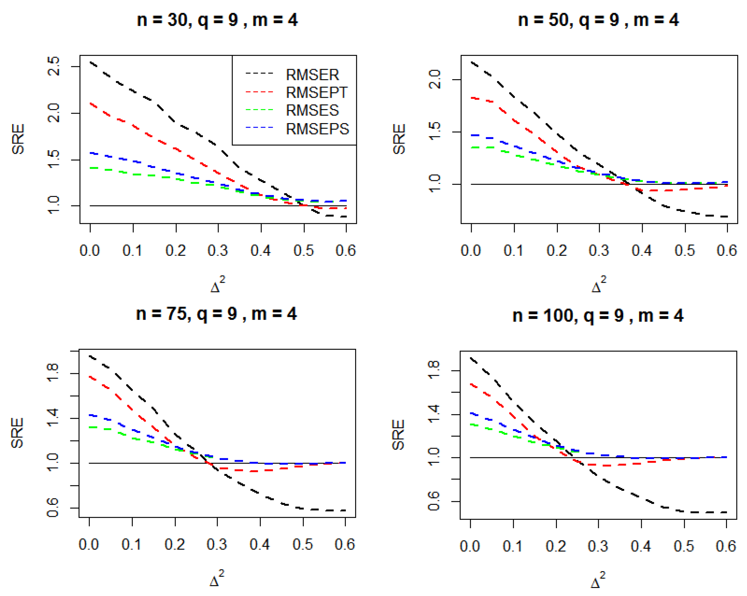
• Compute the simulated relative efficiency (SRE) as follows

  $$SRE({\widehat{\mathit{\theta }}}^U,\widehat{{\mathit{\theta }}^{\ast }})=\frac{SMSE({\widehat{\mathit{\theta }}}^U)}{SMSE(\widehat{{\mathit{\theta }}^{\ast }})},$$

  (29)

  where ${\widehat{\mathit{\theta }}}^U$ is appointed as benchmark. A value greater than one of the $SRE({\widehat{\mathit{\theta }}}^U,\widehat{{\mathit{\theta }}^{\ast }})$ indicates that $\widehat{{\mathit{\theta }}^{\ast }}$ performs better than ${\widehat{\mathit{\theta }}}^U$ and vice versa.

Results of these simulations are reported in Figure 1, Figure 2, Figure 3 and Figure 4. The numerical results effectively assure our analytical results that the positive shrinkage estimator plays the role of a safeguard against the high risks associated with the reduced model that we obtained under the set of local alternatives. ${\widehat{\mathit{\theta }}}^R$ shows the best performance under the null space and it degrades towards zero as the value of ${\Delta }^2$ goes way from the null space.

As the value of ${\Delta }^2$ increases, the superiority changes from ${\widehat{\mathit{\theta }}}^R$ to ${\widehat{\mathit{\theta }}}^{PT},{\widehat{\mathit{\theta }}}^S$ and ${\widehat{\mathit{\theta }}}^{S+}$, respectively, and ${\widehat{\mathit{\theta }}}^{S+}$ dominates other estimators, because it acts as a safeguard against the high risks associated with the reduced model.

6.2. Application on Standard & Poor 500 (SP500) Stock Market

The “sp500dge” dataset contains daily closing prices of the Standard & Poor 500 (SP500) stock market that has been used by Ding et al. (1993). The dataset is also available in fGarch/R-package produced by Wuertz and Chalabi (2008). Following the illustrative example of Ding et al. (1993), we considered the most recent returns as our targeted subset from 3 December 1988 to 30 August 1991. This contains 1000 daily returns (i.e., the official working days in the financial market is 252).

To fit the ARCH model, we first conducted a Lagrange–Multiplier (LM) test to check the effect of ARCH; more details about this test can be found in Tsay (2005). Then, we fit an ARCH model with an adequate order. The order $q=12$ is an adequate selection for our data which represents the full model that given by Formula (30). ${\widehat{\mathit{\theta }}}^U$ is then obtained by fitting the full model.

$$\sqrt{y_t}={\sigma }_t{ϵ}_t,{ϵ}_t\sim N(0,1),{\sigma }_t^2=\omega +{\alpha }_1{y}_{t-1}+\cdots +{\alpha }_q{y}_{t-q}.$$

(30)

In order to obtain the UPI from the data, we used AIC and BIC selection criteria to pick the significant order under the forward selection strategy the selected order under the auxiliary information of AIC and BIC represents the reduced model given by Formula (31). Consequently, from the reduced model, we compute ${\widehat{\mathit{\theta }}}^R$, the restricted estimator.

$$\sqrt{y_t}={\sigma }_t{ϵ}_t,{ϵ}_t\sim N(0,1),{\sigma }_t^2=\omega +{\alpha }_1{y}_{t-1}+\dots +{\alpha }_{q-m+1}{y}_{t-q-m+1}.$$

(31)

To assess the performance of the estimators, we use the relative efficiency of the mean squared error (RMSE) with respect to the true parameters $\mathit{\theta }$ which will be estimated by ${\widehat{\mathit{\theta }}}^{\ast }$, where ${\widehat{\mathit{\theta }}}^{\ast }$ can be any of the estimators. The approach is based on the bootstrapping method which is similar to that introduced by Freedman (1981).

After fitting the full model on the original data, the procedure is conducted in two steps. The first step is as follows:

• Select a sample of size n from the residuals of the full model, say $E_1,\dots ,E_n$ with replacement.
• Compute the observations $Y_1^{\ast },\dots ,Y_n^{\ast }$ as follows

  $$Y_i^{\ast }={\widehat{Y}}_i+E_i,i=1,\dots ,n,$$

  (32)

  where ${\widehat{Y}}_i$ is the ith fitted observation from the full model applied on the original data, and $E_i$ is the ith residual in (1).
• Fit the ARCH model on $Y_i^{\ast }$ to obtain ${\widehat{\mathit{\theta }}}_{boot}^U(1)$.
• Repeat steps (1)–(3) a number of times K until stable results are obtained—we found that $K=3000$ worked well.
• Compute the average of K iterations which will represent the true parameter $\mathit{\theta }$.

After the true parameters’ vector has been estimated in the previous step, the second step is conducted as follows:

• Select a sample of size n from the residuals of the full model, say $E_1,\dots ,E_n$ with replacement.
• Compute $Y_1^{\ast },\dots ,Y_n^{\ast }$ as follows

  $$Y_i^{\ast }={\widehat{Y}}_i+E_i,i=1,\dots ,n,$$

  (33)

  where ${\widehat{Y}}_i$ is the ith fitted observation from the full model applied on the original data and $E_i$ is the ith residual in (1).
• Fit both the full and reduced models and compute ${\widehat{\mathit{\theta }}}_{boot}^U(1)$ and ${\widehat{\mathit{\theta }}}_{boot}^R(1)$, then obtain ${\widehat{\mathit{\theta }}}_{boot}^{PT}(1)$, ${\widehat{\mathit{\theta }}}_{boot}^S(1)$ and ${\widehat{\mathit{\theta }}}_{boot}^{S+}(1)$.
• Compute the predicted values ${\widehat{Y}}_i^{\ast }$ using the estimated parameters of all estimators

  $${\widehat{Y}}_i^{\ast }(1)=X{\widehat{\mathit{\theta }}}_{boot}(1),$$

  where ${\widehat{\mathit{\theta }}}_{boot}^{\ast }(1)\in \{{\widehat{\mathit{\theta }}}_{boot}^U(1),{\widehat{\mathit{\theta }}}_{boot}^R(1),{\widehat{\mathit{\theta }}}_{boot}^{PT}(1),{\widehat{\mathit{\theta }}}_{boot}^S(1),{\widehat{\mathit{\theta }}}_{boot}^{S+}(1)\}.$
• Compute the Bootstrapping Mean Squared Error (MSEB) of ${\widehat{\mathit{\theta }}}_{boot}^{\ast }(1)$ the estimator ${\widehat{\mathit{\theta }}}^{\ast }$ as follows:

  $$MSEB{\widehat{\mathit{\theta }}}_{boot}^{\ast }(1)=\sum _{i=1}^n{({\widehat{\mathit{\theta }}}_{boot}^{\ast }(1)-{\widehat{\mathit{\theta }}}^{\ast })}^2.$$

  (34)
• Repeat steps (1)–(5) a number of times K until stable results are obtained. We found that $K=3000$ is an adequate number of iterations.
• Compute the relative efficiency of the mean squared error (RMSE) as follows,

  $$RMSE({\mathit{\theta }}^{\ast })=\frac{\mathrm{Average}\mathrm{of}\mathrm{MSEB}\mathrm{for}{\widehat{\mathit{\theta }}}^U}{\mathrm{Average}\mathrm{of}\mathrm{MSEB}\mathrm{for}{\widehat{\mathit{\theta }}}^{\ast }}.$$

  (35)

Results of the RMSEs for our data are reported in

Table 1. Relative MSE with respect to ${\widehat{\mathit{\theta }}}^U$ for the S&P500 stock market daily closing prices.

Estimator	${\widehat{\mathit{\theta }}}^{\mathit{R}}$	${\widehat{\mathit{\theta }}}^{\mathbf{PT}}$	${\widehat{\mathit{\theta }}}^{\mathit{S}}$	${\widehat{\mathit{\theta }}}^{\mathit{S}+}$
MSE	1.1236	1.0010	1.0236	1.0382

.

It is clear that ${\widehat{\mathit{\theta }}}^R$ outperforms all other estimators which indicates that the restriction given by the null hypothesis is correct. ${\widehat{\mathit{\theta }}}^{S+}$ comes the second and then it is ${\widehat{\mathit{\theta }}}^S$. ${\widehat{\mathit{\theta }}}^{PT}$ performs better than ${\widehat{\mathit{\theta }}}^U$ even though it was the worst among other estimators. This may be an indication that the AIC/BIC selection criteria worked quite well on this dataset.

7. Conclusions

In this article, we investigated the performance of the pretest and James–Stein (shrinkage) estimators to estimate the parameter’s vector $\mathit{\theta }$ of the ARCH model. These estimators were first analytically compared via their asymptotic quadratic risk and asymptotic mean square error matrices and then numerically compared using simulated and real datasets to confirm our analytical results. However, the reduced model in some cases might not be the right choice: analytical and numerical results showed that the pretest and James–Stein estimators represent a safeguard against the high risks associated with the reduced model that we obtain under the set of local alternatives.

Historically, the ARCH model is the simplest version of ARCH family models; however, its drawback is that it requires many parameters to adequately describes the volatility of such phenomena, and the positive James–Stein estimator should successfully overcome this dilemma by providing a parsimonious submodel (reduced model). To obtain a UPI, we used AIC and BIC selection criteria to select the reduced model.

According to our research findings, it is recommended that the positive James–Stein estimator is used as it outperforms all other estimators regardless of whether the restriction given by the null hypothesis is true. In addition, the proposed estimation strategy can be applied to different ARCH family models.

References

- Ahmed, S. Ejaz, Abdulkadir Hussein, and Marwan Al-Momani. 2015. Efficient estimation for the conditional autoregressive model. Journal of Statistical Computation and Simulation 85: 2569–81. [Google Scholar] [CrossRef]
- Ahmed, S. Ejaz, and Bahadır Yüzbaşı. 2016. Big data analytics: Integrating penalty strategies. International Journal of Management Science and Engineering Management 11: 105–15. [Google Scholar] [CrossRef]
- Ahmed, S. Ejaz, and Bahadır Yüzbaşı. 2017. High dimensional data analysis: Integrating submodels. In Big and Complex Data Analysis. Cham: Springer, pp. 285–304. [Google Scholar]
- Ahmed, S. Ejaz, and Enayetur Raheem. 2012. Shrinkage and absolute penalty estimation in linear regression models. Wiley Interdisciplinary Reviews: Computational Statistics 4: 541–53. [Google Scholar] [CrossRef]
- Ahmed, S. Ejaz. 2014. Penalty, Shrinkage and Pretest Strategies: Variable Selection and Estimation. Berlin and Heidelberg: Springer. [Google Scholar]
- Akaike, Hirotugu. 1974. A new look at the statistical model identification. IEEE Transactions on Automatic Control 19: 716–23. [Google Scholar] [CrossRef]
- Al-Momani, Marwan, Abdulkadir Hussein, and S. Ejaz. Ahmed. 2016. Penalty and related estimation strategies in the spatial error model. Statistica Neerlandica 71: 4–30. [Google Scholar] [CrossRef] [Green Version]
- Al-Momani, Marwan, Syed Ejaz Ahmed, and Abdul A. Hussein. 2019. Efficient Estimation Strategies for Spatial Moving Average Model. In BiometricsProceedings of the Thirteenth International Conference on Management Science and Engineering Management. Cham: Springer, pp. 520–43. [Google Scholar]
- Bancroft, Theodore Alfonso. 1944. On biases in estimation due to the use of preliminary tests of significance. The Annals of Mathematical Statistics 15: 190–204. [Google Scholar] [CrossRef]
- Brockwell, Peter J., and Richard A. Davis. 2016. Introduction to Time Series and Forecasting. New York: Springer. [Google Scholar]
- Dawod, Abdaljbbar, Marwan Al-Momani, and Saddam Akber Abbasi. 2018. On efficient estimation strategies in monitoring of linear profiles. The International Journal of Advanced Manufacturing Technology 96: 3977–91. [Google Scholar] [CrossRef]
- Ding, Zhuanxin, Clive W. J. Granger, and Robert F. Engle. 1993. A long memory property of stock market returns and a new model. Journal of Empirical Finance 1: 83–106. [Google Scholar] [CrossRef]
- Emmert-Streib, Frank, and Matthias Dehmer. 2019. High-Dimensional LASSO-Based Computational Regression Models: Regularization, Shrinkage, and Selection. Machine Learning and Knowledge Extraction 1: 359–83. [Google Scholar] [CrossRef] [Green Version]
- Engle, Robert F. 1982. Autoregressive conditional heteroscedasticity with estimates of the variance of united kingdom inflation. Econometrica: Journal of the Econometric Society 50: 987–1007. [Google Scholar] [CrossRef]
- Francq, Christian, and Jean-Michel Zikoïan. 2004. Maximum likelihood estimation of pure garch and arma-garch processes. Bernoulli 10: 605–37. [Google Scholar] [CrossRef]
- Francq, Christian, and Jean-Michel Zikoïan. 2010. Garch Models: Structure, Statistical Inference and Financial Applications. Hoboken: John Wiley & Sons. [Google Scholar]
- Francq, Christian, and Jean-Michel Zakoïan. 2012. Strict stationarity testing and estimation of explosive and stationary generalized autoregressive conditional heteroscedasticity models. Econometrica 80: 821–61. [Google Scholar]
- Freedman, David A. 1981. Bootstrapping regression models. The Annals of Statistics 9: 1218–28. [Google Scholar] [CrossRef]
- Grublytė, Ieva, Donatas Surgailis, and Andrius Škarnulis. 2017. Qmle for quadratic arch model with long memory. Journal of Time Series Analysis 38: 535–51. [Google Scholar] [CrossRef]
- Hansen, Lars Peter. 1982. Large sample properties of generalized method of moments estimators. Econometrica: Journal of the Econometric Society 50: 1029–54. [Google Scholar] [CrossRef]
- Neter, John, Michael H. Kutner, Christopher J. Nachtsheim, and William Wasserman. 1996. Applied Linear Statistical Models. Chicago: Irwin Chicago, vol. 4. [Google Scholar]
- Peiris, Ushan, and T. S. G. Peiris. 2011. Measuring stock market volatility in an emerging economy: Empirical evidence from the colombo stock exchange (CSE). In International Research Conference. Durgapur: University of Kelaniya-Sri Lanka. [Google Scholar]
- Rathnayaka, R. M., D. M. Seneviratne, and S. C. Nagahawatta. 2013. Statistical techniques approach for evaluating the market fluctuations; the case study in colombo stock exchange. In International Conference on Business & Information. Durgapur: University of Kelaniya-Sri Lanka. [Google Scholar]
- Rich, Robert W., Jennie Raymond, and John Scott Butler. 1991. Generalized instrumental variables estimation of autoregressive conditional heteroskedastic models. Economics Letters 35: 179–85. [Google Scholar] [CrossRef]
- Saleh, A. K. Md Ehsanes. 2006. Theory of Preliminary Test and Stein-Type Estimation with Applications. Hoboken: John Wiley & Sons, vol. 517. [Google Scholar]
- Schwarz, Gideon. 1978. Estimating the dimension of a model. The Annals of Statistics 6: 461–64. [Google Scholar] [CrossRef]
- Stein, Charles. 1966. An approach to the recovery of interblock information in balanced incomplete block designs. In Research Paper in statistics: Festschrift for J. Neyman. London: Wiley, pp. 351–66. [Google Scholar]
- Stein, Charles. 1956. Inadmissibility of the usual estimator for the mean of a multivariate normal distribution. In Volume 1 Contribution to the Theory of Statistics, Proceedings of the Third Berkeley Symposium on Mathematical Statistics and Probability. Berkeley: University of California Press, vol. 1, pp. 197–206. [Google Scholar]
- Teräsvirta, Timo. 2009. An introduction to univariate garch models. In Handbook of Financial Time Series. Berlin and Heidelberg: Springer, pp. 17–42. [Google Scholar]
- Thomson, T., S. Hossain, and M. Ghahramani. 2016. Efficient estimation for time series following generalized linear models. Australian & New Zealand Journal of Statistics 58: 493–513. [Google Scholar]
- Tsay, Ruey S. 2005. Analysis of Financial Time Series. Hoboken: John Wiley & Sons, vol. 48. [Google Scholar] [CrossRef]
- Wang, Changlin. 2021. Different garch models analysis of returns and volatility in bitcoin. Data Science in Finance and Economics 1: 37–59. [Google Scholar] [CrossRef]
- Weiss, Andrew A. 1986. Asymptotic theory for arch models: Estimation and testing. Econometric Theory 2: 107–31. [Google Scholar] [CrossRef] [Green Version]
- Wuertz, Diethelm, and Yohan Chalabi. 2008. fgarch: Rmetrics-Autoregressive Conditional Heteroskedastic Modelling, r Package Version 290.76. Available online: https://www.rmetrics.org (accessed on 3 April 2022).
- Yüzbaşı, Bahadır, and S. Ejaz Ahmed. 2020. Ridge Type Shrinkage Estimation of Seemingly Unrelated Regressions Furthermore, Analytics of Economic and Financial Data from “Fragile Five” Countries. Journal of Risk and Financial Management 13: 131. [Google Scholar] [CrossRef]