Article

Time Dependence of CAPM Betas on the Choice of Interval Frequency and Return Timeframes: Is There an Optimum?

Maine Business School, University of Maine, 5723 D. P. Corbett Business Building, Orono, ME 04469, USA
*
Author to whom correspondence should be addressed.
J. Risk Financial Manag. 2022, 15(11), 520; https://doi.org/10.3390/jrfm15110520
Submission received: 12 October 2022 / Revised: 31 October 2022 / Accepted: 1 November 2022 / Published: 7 November 2022
(This article belongs to the Special Issue Mathematical and Empirical Finance)

Abstract

:
The traditional CAPM beta is almost exclusively calculated over a return period that spans a window length of 60-months, at one-month return frequencies. It is one of the most utilized models in the asset management industry to assess systematic risk. Yet there is limited evidence to suggest that these estimation parameters are optimal. Utilizing data between January 2000 and December 2021 for the Russell 1000 index, we test daily, weekly, and monthly beta estimations to calculate tracking errors (TE) for the use of these betas in predicting subsequent performance over daily, weekly, and monthly timeframes. We identify that daily CAPM betas are best for predicting subsequent period daily returns and that weekly CAPM betas are strongly correlated with forward weekly and monthly period returns. Leveraging the significant advances in computing resources and the increasing utilization of high frequency trading strategies, we argue that additional window length and return interval-based CAPM betas should be calculated for estimating the systematic risk embedded in diversified portfolios.

1. Introduction

The assertion that there is a relation between portfolio beta and the market return has been analyzed and debated for decades. The Sharpe-Linter-Black CAPM model (1964) supports this theory and states that the expected return is a positive linear function of beta, the risk free rate and the expected market return, while other researchers question the usefulness of the beta in predicting the expected return. More recently, Lin (2021) tested the consistency of a five-factor process as applied to an intertemporal CAPM model. Fama and French (1992) asserted that there is no systematic relationship between beta and security returns. Some others agree on the relationship but introduce non-linearity in the relationship (Carroll and Wei 1988). Chen et al. (1986) argued in favor of measuring the relationship between security expected returns using several macroeconomic variables. Lakonishok and Shapiro (1986) presented the case that there is empirical evidence that security returns are affected by an unsystematic risk component. Hollstein et al. (2020), in a recent study, find that intra-day high frequency return-based betas explain the size anomaly better than the conditional betas based on daily returns.
With all these differing and evolving views on the validity of the CAPM beta, a practitioner still cannot look beyond the fact that the traditional CAPM beta remains one of the most widely used factors in the capital markets. According to Graham and Harvey (2001) in a survey of industry participants, over seventy percent of respondents always or almost always look at the traditional CAPM beta, especially when it comes to assessing the extent of systematic risk in the portfolio.
The CAPM model, however, does not give any guidance into whether the beta should be measured daily, weekly, monthly, quarterly, or annually (Roman and Terraza 2018). The beta coefficient of a security will vary across different return frequencies. The phenomenon is referred to as the intervalling (or intervaling) effect bias in beta (Hawawini 1980; Fung et al. 1985; Corhay 1992). CAPM modeling also does not indicate the optimal regression window length that should be utilized to estimate betas. With a longer estimation window (greater than, say, 24 or 60 months) there are more observations in the regression; however, going much further back could introduce issues related to a transformed company with a different set of characteristics, even though it remains under the same company name (or CUSIP number as in the CRSP Pricing database 2022); this can happen when a larger company merges with others over time.
The purpose of this study is not to argue the validity of the CAPM model or its linearity, it is rather to answer the question of what is the optimal interval period (of returns) and window-length of estimation that would yield a beta estimate, whose utilization would make the daily, weekly, or monthly estimation and forecast of systematic portfolio risk more robust. The quantitative community in the US asset management industry primarily uses vendor-supplied betas, which are based on a 60-month return calculation (monthly interval frequency combined with a 60-month window-length of estimation period). We think that there is a legacy issue here, borne out of computational and data limitations years ago (Sharpe 1964) when beta first started getting deployed en masse in industrial portfolio evaluation.1 These considerations do not exist at the time of writing of this research. The impact of in-the-money vested options, warrants or other convertible securities on EPS dilution was first systematically documented by Goldsticker and Agrrawal (1999), subsequently Akono et al. (2019) found that Regulation FD was partially successful at curbing the influence of management incentives on analysts’ research when signaling expected underperformance by way of rounding to zero the EPS estimates; nonetheless such EPS volatility then feeds into stock valuation volatility, eventually resulting in unstable betas. As will be shown in the results, stocks with higher volatility are increasingly sensitive to varying frequency and estimation window lengths.
A survey of literature did not turn up any substantial/formalized insights into what is the effect of changing the interval of returns (monthly, weekly, and daily frequency of returns) on the traditional CAPM beta calculation, or the impact of altering the window-length (apart from the traditional 60-month window) on the accuracy/stability of the CAPM beta’s prediction of the forward one-day return. In particular, there appears to be no justification to employing a 60-month beta, based on monthly return intervals to indicate/estimate a one-day or one-week portfolio systematic risk. We also think that with the growth of the market-neutral hedge fund industry, the need for daily portfolio rebalancing may necessitate the use of differing interval betas, with a drift towards higher frequency information (Hollstein et al. 2020), and thus shorter intervals.

2. Literature Review

The literature on the impact of ‘intervalling’ and window length variation on CAPM beta estimation is somewhat intermittent, though deep. Most of the work discusses the effect of different intervals on the return distributions and dispersion of residuals. Hollstein et al. (2020), find that intra-day high frequency return-based betas explain the size anomaly better than the conditional betas based on daily returns. Hawawini (1980), in his seminal paper on the intervalling effect, demonstrated “mathematically that the skewness of securities’ returns—the ratio of the third moment to the standard deviation cubed—is sensitive to the length of the differencing interval over which returns are measured.” In his paper, he demonstrates that “the higher the moment’s order, the more sensitive it is to the length of the differencing interval over which securities’ returns are measured.” Smith (1978) estimated the “characteristic lines of 200 common stocks (are examined) over the period 1950–1969. With respect to measurement, geometric mean return decreased slightly and predictably with intervalling. The dispersion of return distributions decreased with longer intervals. Return distributions exhibited positive skewness. Goodness-of-fit for characteristic lines improved with the use of longer intervals. Estimates of beta increase with intervalling for aggressive stocks.” These studies apply the Gaussian distribution to the return random variable x, with the mean and standard deviation of the distribution denoted by μ, σ respectively.
f ( x ) = 1 σ 2 π e 1 2 ( x μ σ ) 2
The cumulative distribution function (CDF) of a standard normal distribution with μ = 0, σ = 1 is the integral of the PDF given above from minus infinity to a value of z and is given by:
Φ ( z ) = 1 2 π x e x 2 / 2   d x
In the area of quantitative financial analysis, the distribution of stock prices (x) is, however, modeled as a log-normal distribution, since x ≥ 0 with parameters μ, σ modified as:
μ = ln ( μ X 2 μ X 2 + σ X 2 )   a n d   σ 2 = ln ( 1 + σ X 2 μ X 2 )
However, when the call option writing is applied to portfolios, the single time unit portfolio returns are no longer normally distributed. Despite the asymmetry of returns introduced by option writing, Buckle (2022) shows that the long-run portfolio returns, in fact, become normally distributed, for any invariant option-adjusted portfolio. For the bivariate (x, y), standard normal distribution (μ = 0, σ = 1) with correlation ρ, the joint PDF is given as:
f ( x , y ) = 1 2 π σ X σ Y 1 ρ 2 exp ( 1 2 ( 1 ρ 2 ) [ ( x μ X σ X ) 2 2 ρ ( x μ X σ X ) ( y μ Y σ Y ) + ( y μ Y σ Y ) 2 ] )
Hawawini and Vora (1980) find that there is a consistent pattern of leads or lags for securities’ daily returns and it does not hold over monthly returns for securities traded on the NYSE and the AMEX. Girard and Sinha (2006) explore the risk premiums and time varying covariance structures in emerging markets and find that their response mechanisms are not just linked to the local risk factors. Global ETFs can be easily deployed to produce efficient portfolios in a multi-asset mean-variance optimized framework (Agrrawal 2013), who demonstrated that a multi-asset six ETF global portfolio can have 30% less systematic risk (beta) than a pure equity index, such as the S&P 500. Reilly and Wright (1988) noticed discrepancies in published betas estimated over the same five-year period and conducted a factorial analysis of variance to test whether the betas were indeed statistically different. They concluded that: “1. the main reason for observed variation between published betas is the interval effect, and 2. the security market value is a significant predictor of the magnitude and the direction of the difference.” The predictive ability of the varying interval betas was, however, not explored in their paper.
Corhay (1992) studied 250 domestic securities traded on the spot market of the Brussels Stock Exchange from January 1977 through December 1985 and noted that “an important issue related to the systematic risk or beta coefficient of a security is its sensitivity to the length of the differencing interval used to measure the returns. The results indicate that an intervalling effect bias is present in the estimated security betas for short differencing intervals. The bias in the betas is very important, especially for small market value securities, and it decreases when the differencing interval used to measure the returns is lengthened. The results also demonstrate that small firms have, on average, lower beta coefficients than large firms.2
Corhay and Rad (1993) finds that in a sample of 50 thinly trading Dutch stocks the “beta estimates from short intervals are on average lower than those obtained from longer intervals” and that there is variability in the coefficients for varying interval lengths. The Corhay (1992) study has its focus on the matter of asynchronous trading and the problems that such non-overlapping estimation windows introduce into robust beta estimation.3
Groenewold and Fraser (2000) discuss that CAPM betas are generally estimated from historical data using a “5-year rule of thumb” and explore their ability to correlate with subsequent period returns. They estimate various “time-varying beta” regression models, which are then subsequently used for forecasting. They report that, “forecasting equations have good explanatory power but that their forecasts are dominated, on average, by the 5-year rule of thumb.” Levy et al. (2001) report that there is a pronounced impact on the regression and “even a shift from weekly data to quarterly data affects the regression coefficient substantially.” They analyze this in a multiplicative-additive framework of creating sub-periods (intervals) from the available period. Ho and Tsay (2001) find that for small-cap stocks, the downward bias in beta estimates diminishes once options are listed on the underlying stock, indicating that the price-adjustment process mitigates the intervalling effect, which is pronounced with smaller-sized stocks. Armitage and Brzeszczynski (2011) found a downward bias in daily betas as a result of the higher idiosyncratic component in daily returns (manifesting in heteroscedasticity of the error term). Intraday volatility is an increasingly impactful factor that creates bias in risk measures (Fang et al. 2012); hence, the assumption that a single beta estimation method would be universally applicable to different portfolio styles may not yield optimally. Mantsios and Xanthopoulos (2016) found a significant intervalling effect in the outcomes of the betas of stocks traded on the Athens Stock Exchange during their 2007–2012 economic crisis. Jurdi and AlGhnaimat (2021) find that firm-level variables such as size, leverage, dividend payments, and diversification impact firm total risk and thus beta. Abate et al. (2022) utilize monthly returns in their constrained optimization models to arrive at efficient allocations. The liquidity of prominent ETFs and its primary drivers have been evaluated in Agrrawal et al. (2014).

3. Data and Methodology

For our stock universe, Russell 1000, which we examined using the test period from 1 January 2000 through 31 December 2021 (CRSP via WRDS 2022), the first beta calculations involve estimation windows that end on 31 December 2021. The top 1000 of stocks on US exchanges comprise about 92% of the total market cap of all listed stocks in the U.S. equity market. Our WRDS/CRSP dataset provided us with CRSP tracked firms incorporated in the US and listed on the NYSE, AMEX, or NASDAQ that have a CRSP share code of 10 or 11 at the beginning of month t, extracted from the WRDS/CRSP files. The survivorship bias free portfolio formation is conducted over the period of 2000–2021. Betas are endogenously calculated using the standard market model (Equations (1)–(4), next section). The results of our work are not state dependent on say a unique set of macro, geo-political, or interest rate regimes (such as pre or post the Bretton Woods currency/gold standard agreement (Eichengreen 2021)). There could be future research conducted to compare indexes, such as the Russell 3000, the Wilshire 5000 and then to the Morgan Stanley MSCI international EAFE Index and see whether there are places where the optimal Beta window is more or less pronounced while calculating the subsequent tracking errors. Extending it back in time would further indicate that the frequency effect and intervaling matching spans time. Cremers and Petajisto (2009), in their seminal paper on suggesting a modification to the Fama and French (1992) paper, use return data that is over the 1980–2003 period. Additionally, the results we find are invariant year over year, and a priori we expect they will stay that way over previous time frames, since it is only a methodological readjustment that we have introduced.
Our purpose is to determine whether different criteria employed in the calculation of the beta lead to a better predictive ability of subsequent portfolio returns. In this paper, we examine two dimensions in the computation of portfolio betas: the interval length of the returns and the length of the estimation window. The intervals are the return periods used for the comparisons of security returns to the market portfolio. We calculate betas based on daily, weekly and monthly returns. The estimation window is the period of time over which the beta is calculated. The traditional beta calculation uses a monthly interval length and a five-year estimation window (Corhay 1992). If recent systematic risk is deemed more relevant to near term portfolio performance (hedge funds or portfolios with more of a tactical asset allocation approach), then betas with shorter estimation periods might prove more appropriate. We use estimation windows of 1 to 5 years.
Thus, for instance, the first set of betas with a 5-year estimation window were calculated with a start date of 31 December 2016, while the first beta calculations involving 1-year estimation windows had a 31 December 2020 start date. The estimation windows are then run over a loop to produce the vector of betas, with varying return frequencies (D, W, M) and estimation window lengths (1 through 5 years). There are three forward looking time periods for which the tracking errors are calculated (1 day, 1 week and 1 month). The predictive ability of the various calculated betas are then gauged for their effectiveness in explaining subsequent daily, weekly and monthly returns.
The OLS beta for individual securities is estimated with the standard market model, with additional specifications with respect to a time interval of L and a window-length of estimation T.
r i = α i + β i r M + e i
r i L T = α i L + β i L r M L T + e i L T
and;
  • ri is the return on security i
  • rM is the return on the market
  • βi is the calculated beta coefficient
  • αi is the intercept term, and
  • ei is the residual term
For each beta interval length (frequency) and estimation window period, betas are calculated using the two pass OLS return methodology, as listed below (Cohen et al. 1983b). The OLS beta is estimated from the standard market model, with additional specifications with respect to a time interval of L days (implying that the return interval would vary from a daily beta, a weekly return-based beta and a monthly beta). Additionally, we vary the window-length of estimation T, which is sub-divided into a set of periods determined by L and is equal to a rounded integer value of T/L4. Both r i L T and r M L T are continuously compounded returns over the specified interval L, and computed as the difference between the natural logarithms of successive closing prices, adjusted for dividends and corporate action.
β ^ i O L S β i L
r i L T = α i L 1 + β i L 1 r M L T + e i L T 1
β i L 1 = α i 2 + β i 2 f i ( L ) + e i L 2
  • L interval length in days (D, W, M);
  • for each security i = 1, ….. N;
  • and over time T = [ 1 , . , n   days ] / L window   length .
A one-year return period will have 252 trading days.
Portfolios are then formed based on the security betas and market capitalization levels (three fractiles for Large, Mid and Small capitalization groups, since we are operating within the Russell 1000 universe) at that point in time t. EW (Equal Weighted) portfolios when aggregated would have a performance drift from the observable VW (Value Weighted) index return over the same time period [due to the small-cap risk factor manifesting, this was noted in Carhart (1997)] and also by Cremers and Petajisto (2009), who pointed out that in the Fama and French (1992) paper, the sub-portfolio returns were based on equal-weighted returns. Hence, the sub-portfolio returns in this study are value weighted-based, based on the prior period capitalization. The beta-based fraciles are EW (CRSP via WRDS 2022). The actual portfolio returns for the subsequent period (t + 1) were then compared to the expected returns based on the portfolio betas and actual returns of the market. This was conducted for daily (D), weekly (W) and monthly (M) forecast lengths. Then, new betas were calculated with a window estimation period ending one month later; and new portfolio combinations formed. The interval and window-length combinations that yielded the lowest tracking error would provide the preferred beta estimate for each portfolio combination and forecast length (forward 1 day, 1 week or 1 year).
Since the CAPM is more relevant for portfolios, where unsystematic risk has been diversified away and beta is the only relevant measure of the risk in security, the analysis was conducted on a portfolio level rather than an individual security level. We formed various portfolio combinations from the Russell 1000 universe based on market capitalization, beta, as calculated above, and a combination of market capitalization and beta (Table 1 (A, B, C)).
We use the annualized tracking error of forward-looking portfolio return estimates as our measure of the explanatory power of the various beta coefficients. The annualized tracking error, TE, is derived from the standard deviation of differences between the actual and expected portfolio returns, as demonstrated below:
T E = λ t = 1 N ( r P , t + 1 β P r M , t + 1 )
where:
  • N = The total number of periods examined (our current sample has 186 periods);
  • λ = The number of return periods per year (when forecasting daily returns, λ = 252; for weekly returns, λ = 52; and for monthly returns, λ = 12);
  • βP = The equal-weighted portfolio beta based on a given interval and estimation window;
  • rp,t+1 = The actual portfolio return for the period immediately following the beta calculations and portfolio formation;
  • rm,t+1 = The actual return of the Market, as proxied by the total return of the Russell 1000, for the period immediately following the beta calculations and portfolio formation.

4. Results

The estimation of tracking errors for varying time frames (window lengths and interval return frequencies) is discussed in this section. Milonas and Rompotis (2013) examined the intervalling effect bias in a sample of forty ETFs’ systematic risk, as well as the relation between beta and capitalization of ETFs and also the intervalling effect bias in ETFs’ tracking error. They find a positive association between the intervalling effect and tracking error, as well as the return interval. For our set of the Russell 1000 stocks, we compare the tracking errors (Chu and Xu 2021)5 of the various combinations of estimated betas (e.g., 1 year daily, …, 5 year daily, 5 year weekly, 5 year monthly, etc., for a total of twelve such variations).
The following exhibits labeled as, Table 1 (A, B, C) depict forecast windows of 1 day, 1 week and 1 month, respectively (in the rows). We first establish whether there is a particular interval length (daily, weekly or monthly) that generates the highest occurrence of return prediction stability across varying forecast windows, by identifying the cells with the lowest tracking error (TE). Thereafter, the tracking errors of the different combinations of Beta-Size6 groups (twelve such groups) are listed in the successive columns, in each of the tables. The lower the tracking TE, the higher the subsequent period return predictability. This generates a total of 3 rectangular matrices of 15 × 12 dimensions each, thus totaling 540 (180 cells times 3 sets) unique TE’s. We further synthesize these three information matrices (of tracking errors) by distilling the 540 TE cells into a consolidated 3 × 3 classification matrix. That matrix will be presented and discussed after the three core tables that show the TE’s associated with daily, weekly and monthly forward returns, respectively. While the three sub-panels in Table 1 look similar, they differ in the length of the forward return period. For Table 1.A, the cells demonstrate the TE’s associated with a 1 Day forward return; for Table 1.B, the cells demonstrate the TE’s associated with a 1 Week forward return; for Table 1.C, the cells demonstrate the TE’s associated with a 1 Month forward return. These are a few TE horizons for institutional portfolio managers with varying risk mandates. The lowest TE (most desirable) is highlighted for each column. In each case, the TE is between the observed forward return and the estimated portfolio return based on βP, the portfolio beta based on a given interval and estimation window. The objective is to test the efficacy of varying interval and frequency betas in estimating portfolio returns that would most closely align with next period of returns (which could be 1 Day, 1 Week or 1 Month, the results of which are in Table 1 (A, B, C) [Combined Table 1].
The tables above are highly condensed output, derived from a large set of return numbers (three different return frequencies, for 1000 stocks per year and over a twenty-year period, with overlapping window length regressions), so that the reader can focus on the core findings. In order to further distill and simplify the embedded information in Table 1, we subsequently reduce the 15 × 12 matrix comprising of 540 cells and 3 sub-matrices, into a 3 × 3 Classification matrix.7
This is accomplished by first flagging the minimal TE value across each Beta-Size combination within each forecast window—this step reduces the 180-cell matrix to a 12-element array (one minimum TE value for each column). The second step involves aggregating each of the ‘minimal’ TE’s across one of the three interval lengths used in the beta estimation, irrespective of the window-length utilized. As an example, the ‘Daily 3 Years’ and the ‘Daily 4 Years’ beta series would be classified under ‘Daily Betas’ interval length (in the classification matrix shown here), and the number of minimal TE’s occurring within the daily beta panel be noted. A total of 36 minimal TE occurrences are thus classified for accuracy.
Each cell lists the number of occurrences a minimum TE was observed for the beta~forecast length combination, as listed in Table 1 (A, B, C). A few inferences and deductions from Table 2 are in order. It appears that there is an observable overlap between interval length and forecast window length, particularly for the daily and the weekly settings. While the classical CAPM gives us little guidance on this matter, we do find some indications, which appear to be intuitively justified, that daily beta-based portfolio returns would be the most correlated with next period daily returns. While nine of the twelve daily forecast returns with minimum TE were attributable to daily interval betas (3 × 3 matrix cell a1), only four of the twelve monthly forecast returns with minimum TE were attributable to monthly interval betas (cell c3). In fact, it may be possible that weekly interval betas are more robust predictors of 1-month ahead returns (6 of the 12 occurrences; cell in b2).
For daily return forecasting, the use of betas estimated by utilizing daily returns appears to be the interval of choice; 75% (nine of the twelve TE’s)8 of the daily beta and 1 day forecast return combinations had minimal TE’s when using daily betas for daily return estimation. Apart from the fact that monthly betas appear to have limited monthly return predictability, we also notice that there is only one occurrence within monthly betas that generates a minimal TE in predicting 1-day ahead returns. In other words, the use of monthly betas to forecast daily portfolio returns does not seem to be a good approach (long-short market neutral hedge funds can have very short performance attribution periods, as an example).
The diagonals on the classification matrix also indicate that for daily and weekly single period forecasts, the returns based on daily and weekly interval betas would have greater accuracy. As such, these that tables provide metrics that indicate that the generally witnessed practice of utilizing a monthly interval beta (over a 60-month estimation period) to estimate next day portfolio returns or to control for portfolio risk in a market-neutral setting, may not be optimal.
Parametric and non-parametric tests for equality of means, medians and variances reject the null hypotheses of equality between the three types of betas (daily, weekly and monthly) are presented in Table 3. Apart from the Kruskal–Wallis and Welch F-tests, we also utilize the Levene’s (1960) test for group variance equality. The formulation for Levene’s W = ( N k ) ( k 1 ) i = 1 k N i ( Z i Z ) 2 i = 1 k j = 1 N i ( Z i j Z i ) 2 with Z i j = | Y i j Y i ¯ | where k is the number of different groups to which the sampled cases belong, Ni is the number of cases in the ith group, N is the total number of cases in all groups, and Yi,j is the value of the measured variable for the jth case from the ith group. The variance increase (Armitage and Brzeszczynski 2011) can also be observed in Figure 1 and is noticeable for betas above the 2.0 level.
Parametric and non-parametric tests for equality of means, medians and variances reject the null hypotheses of equality between the three types of betas (daily, weekly and monthly). While the Kruskal–Wallis and Welch F-test are standard tests, we utilize the Levene’s (1960) test for group variance equality, given that our return series are based on varying periodicity. The variance escalation can also be observed in Figure 1 and is noticeable for betas above the 2.0 level.
The dispersion of betas is higher for the monthly frequency betas and is concentrated towards values β > 2.25. Values of β < 0.5 also show some dispersion for the weekly and daily series. This is also observed in the fat tails of the histograms shown in Figure A1, Appendix A. Figure 2 has a surface plot rendition of the varying interval beta series, below:
The frequency of returns does seem to impact the estimated beta values and the 1-period forward return tracking errors. In Figure 3, we observe that of the three types of betas, the one using the weekly return frequency has, for most market capitalization groups, the lowest tracking error for 1-period forward returns (higher bars are better). The ‘purple’ colored bars are for the Large Cap stocks and have the highest occurrence of the lowest observed tracking errors, especially for the weekly return series and for the 3-, 4- and 5-year estimation period. The 1-year and 2-year window length estimation period yields the most unstable betas, particularly for the daily and monthly return frequencies (lowest occurrence of low TE’s). The ‘maroon’ colored bars are for Mid Cap stocks and have the highest occurrence of the lowest observed tracking errors for the daily return series (3 and 4 year) estimation periods. Figure A1 and Figure A2, in the Appendix A provide a visual representation of the distribution of the three beta series and their overlap densities.
The primary driver for very short-term volatility is systematic risk, as most of the high frequency data pertains to market/economy wide events (Corhay 1992), while idiosyncratic risk is most likely to be triggered by low frequency events (Terraza and Roman 2021). For small-firms, the release of new information is at an even lower frequency. For short differencing intervals (daily), an overlap of the information set used to derive the beta estimates (captured at a higher frequency daily returns) with the return forecasting period, seems to yield better results (lower TE’s) than cross-matched combinations (e.g., monthly forecast period vs. daily betas). Mantsios and Xanthopoulos (2016) also found a significant intervalling effect in the betas of stocks traded on the Athens Stock Exchange during their 2007–2012 economic crisis. Our study finds support for their work, and over a much longer period (2000–2021) in the US equity market.
“Wrong” or rather mismatched optimal windows of beta estimation would result in higher TE (tracking errors). Portfolio managers are likely to increase portfolio turnover with higher TE to reduce volatility with higher levels of trading, but suboptimal beta calibration for their forecast/holding period duration would mean that trading would not be effective. In a perfect world, the beta frequency and estimation window could be customized to observable portfolio holding periods and turnover ratios, to derive the lowest possible tracking errors. However, the turnover would be excessive; hence, we limit the beta frequencies to be D, W and M. We demonstrate that the TEs are higher with mismatched beta frequencies and windows and suggest additional work in the domain, in order to identify and develop mechanisms for PMs to align the beta frequencies/windows (for their risk reports) with their portfolio strategies and turnover.

5. Further Research

To identify and isolate any effect of market directionality on the relationship between interval type, window-length and subsequent period TE, this analysis could be divided into conditional dual periods based on the up and down markets (Pettengill et al. 1995; Cooper 2009).
  • Some preliminary work indicates that, in down markets, it appears that weekly betas accomplish lower TE’s than daily betas. It would be interesting to explore this further, though we do think that the increased volatility witnessed during down-markets may have an association with this observation and that the use of daily betas during bear markets may be too unstable for next day forecasting (Alexeev et al. 2016). With r i and r m D as the excess returns to security i and down market excess returns, respectively, where r m is the full market excess return, then the downside dual beta (Chong 2022) is:
    β = C o v ( r i , r m D | r m D < r m ) V a r ( r m D | r m D < r m )
    The upside dual beta would be of a similar construct but with the inequalities reversed.
  • Given the extensive amount of computational time it took to analyze the time series of returns in their various permutations and combinations, additional work could be undertaken to design an appropriate and efficient scanning mechanism to identify the optimal combinations of interval, window-lengths and the beta-size dimension.
  • The impact of varying intervals and window-lengths on the one-period ahead predictability of systematic risk can alternatively (to the tracking error, TE) be assessed by the Information Coefficient (IC); stable and robust betas will likely result in higher IC’s, but the formal assessment could be a future research item (Appendix B).

6. Conclusions

In this paper, we have empirically considered whether the standard 60-month window length for calculating CAPM betas for portfolios is optimal for all trading interval lengths. Considering the condensed output of 540 cells (of portfolios TE’s) from this study, over the period 2000 to 2021 (three rectangular matrices of 180 cells), we find that forecast interval lengths matched to daily or weekly return-based betas are more likely to lead to the lowest tracking errors. When considering the plurality of options for all types of market capitalizations (large, mid and small), the weekly return frequency performs best in producing the lowest TE for 1-period forward returns. Large Cap stocks have the highest occurrence of the lowest observed tracking errors, especially for the weekly return series. The 1-year and 2-year window length estimation period yields the most unstable betas, particularly for the daily and monthly return frequencies (they have the lowest occurrence of low TE’s). Mid Cap stocks have the lowest tracking errors associated with daily or weekly intervals and estimation window lengths of four and five years. Thus, while there is no optimal combination, the analysis leans towards shorter return intervals (daily or weekly but not monthly) and longer estimation periods (four or five years of returns). This combination can be very intense on computing time, but is nothing compared to the scale of crypto mining and blockchain authentication (Lei et al. 2021; Verhoeven et al. 2018). Results indicate that the generally witnessed practice of utilizing monthly interval betas (over a 60-month estimation period) to estimate next day or next week portfolio returns, or to control for portfolio risk in a market-neutral setting, may not be optimal and is likely a vestige of legacy issues that are no longer relevant (in an era of cloud computing, high frequency data, machine readable data and AI). Agrrawal (2009) demonstrated that pricing data for new firms could be programmatically harvested from the web much before they get archived in a machine-readable format from the larger data providers (WRDS 2022).
A non-overlapping series of betas will result in a more robust tracking error estimation resulting from a matching interval frequency with the forecast period, eventually resulting in greater portfolio stability (less churn, less portfolio turnover and fewer expenses, the benefits of which will eventually percolate to the investor). Given the advent of HFT strategies and also high-volume IPOs, many newly floated companies just do not have 60 months of inception-to-date pricing data. As such, a shorter estimation window but higher frequency (e.g., 18 months of weekly return-based betas, instead of 5-year monthly return-based betas), would still meet the Central Limit Theorem caveats and have sufficient return observations to have usable betas for portfolio risk estimation. Stable and robust betas can result in higher IC’s (information coefficients) and is demonstrated in the Appendix A. That is also a future research item.
Considering the findings herein, and given how common it is for industry participants to consider CAPM betas for portfolio risk estimation, we think that additional research is needed to understand how the interplay between interval frequency and estimation period length impacts the CAPM betas and the resulting tracking errors for investment portfolios. In the age of Fintech and cloud computing, the market participants do not have to have their portfolio risk calibrated by a metric that has mostly served well, but was derived over fifty years ago (Sharpe 1964; Lintner 1965; Black 1972).

Author Contributions

Conceptualization: P.A.; methodology: P.A.; software, MATLAB code and user written VBA, P.A.; validation, P.A.; formal analysis, P.A., F.W.G. and J.H.; investigation, P.A., F.W.G. and J.H.; resources, P.A., F.W.G. and J.H.; data curation, P.A.; writing—original draft preparation, P.A.; writing—review and editing, P.A., F.W.G. and J.H.; visualization, P.A.; supervision, joint F.W.G., J.H. and P.A. All authors have read and agreed to the published version of the manuscript.

Funding

This research received no external funding. No APC was applied to the paper.

Data Availability Statement

Pricing data on stocks. Is via the Wharton Research Data Services. Available online: https://wrds-www.wharton.upenn.edu/ (accessed on 1 March 2022).

Conflicts of Interest

The authors declare no conflict of interest.

Appendix A

Figure A1. Histograms of betas (daily, weekly and monthly return series, 2000–2021).
Jrfm 15 00520 g0a1
The monthly betas have the relatively largest variance (flattest histogram, in green hue), while the daily betas have the lowest variance (blue histogram). A total of 99% of betas are in the [−1, +3] range. Conducting the Jarque-Bera test (Jarque and Bera 1980) for normality J B = n 6 ( S 2 + 1 4 ( K 3 ) 2 ) , indicates that the daily betas have more of a normal approximation than the monthly betas.
Figure A2. Percentile plot of betas (daily, weekly and monthly return series, 2000−2021).
Jrfm 15 00520 g0a2
The percentile plot or CDF (cumulative density function) for the three beta estimates are shown here. The monthly betas (blue CDF line) have a distinct separation from the daily and weekly beta CDFs. This is also observed in the histograms and from the Jarque-Bera test. Percentiles associated with the beta levels can be read directly off the X-Y point of intersection.
Figure A3. Ternary density plot of betas (daily, weekly and monthly return series, 2000–2021).
Jrfm 15 00520 g0a3
We utilize this plot to visually observe that while the three types of beta estimates are clustered with each other, there is a higher level of scatter for the weekly and monthly betas.

Appendix B

To capture the varying of the interval effect, Ho and Tsay, 2001 deployed the following three functional forms. Furthermore, there are varying values of n with a lower bound of zero. Cohen et al. (1983a) find that n = 0.08 produces the best linear fit for the power function.
The negative “n” form is essentially the inverse of the interval length (L):
f ( L ) = L n
and the logarithmic form:
f ( L ) = ln   ( 1 + L n )   and   n > 0
and the exponential function form:
f ( L ) = e L n
The above methodology (Ho and Tsay 2001), provides the distribution of betas with varying interval lengths and window-lengths of estimation.
To obtain the Spearman cross-correlations of the individual security betas for each interval length, the following will populate a symmetric triangular η × λ (where η = λ return periods in the interval) matrix with all diagonal elements equaling 1.
[ 1 1 1 ρ S ( β i L η , β i L λ ) 1 1 ] η x λ   η ,   λ = 1 , 45
If the betas are close to one and significant, it would be indicative of a weak intervalling impact on the ranking of betas across varying interval lengths.
The impact of varying intervals and window-lengths on the one-period ahead predictability of systematic risk can alternatively (to the tracking error, TE) be assessed by the Information Coefficient (IC); stable and robust betas will likely result in higher IC’s, but a formal assessment could be a future research item.
IC s = ρ S ( β i , t L η , r i , t + 1 L λ )
where:
For   each   market   state   s   { R m > R f R m < R f }
  • η ,   λ = 1 , 45   and   η = λ for each T and where t T ,
  • t is a discrete period 1…N within each interval length of size T,
  • rit is the return on each security at time t within each interval T, and
  • IC is the information coefficient.

Notes

1
Advent of firms such as BARRA, Berkeley, 1975 and Vestek Systems, San Francisco, 1983.
2
Does not equate with lower total risk (volatility).
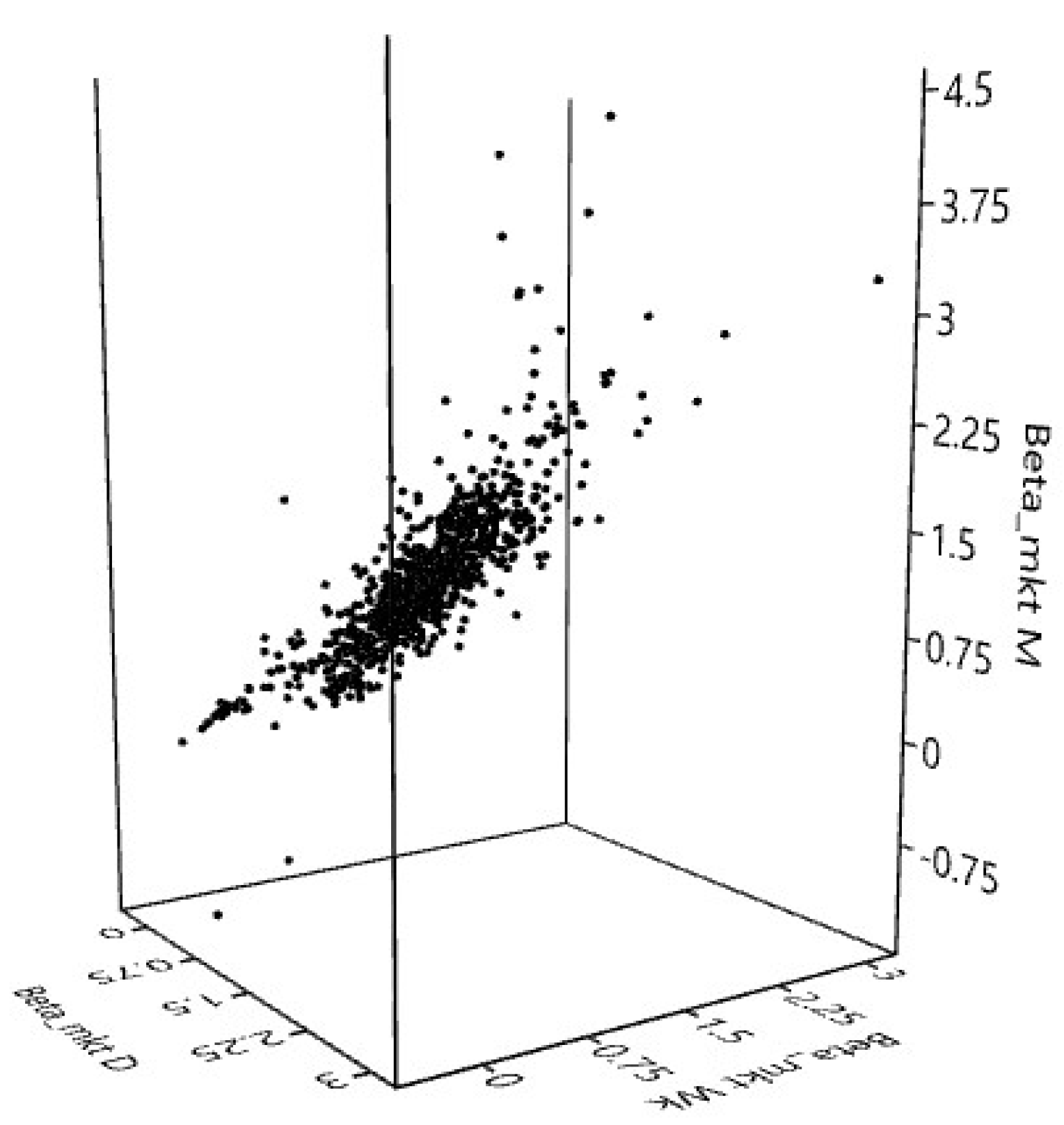
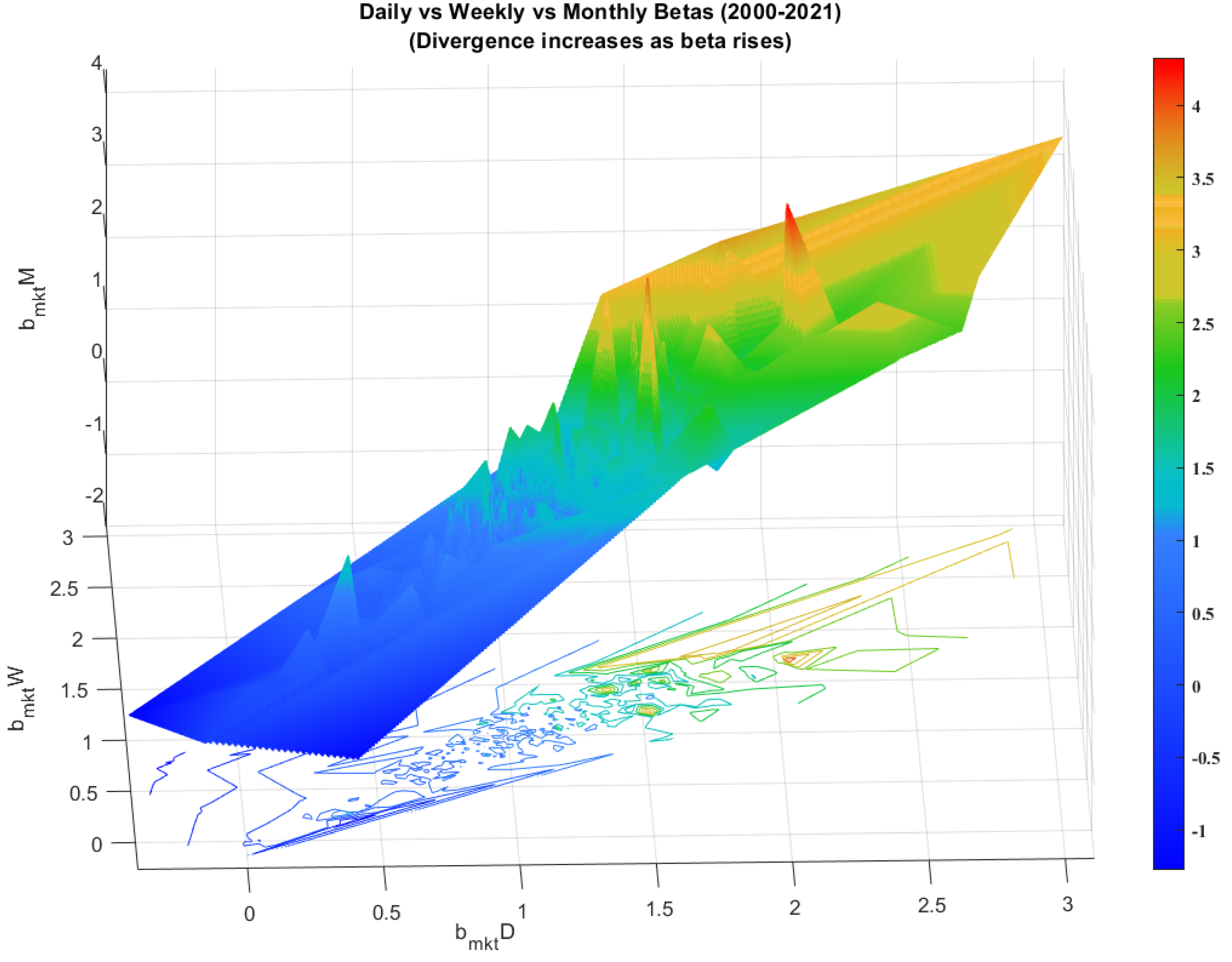
3
The inverse relationship between interval length and average beta values, especially for smaller sized firms is intriguing. Perhaps there is an implicit tradeoff between a downward bias in the estimated beta and its ability to correctly provide an estimate for next period systematic risk. The idiosyncratic component of risk for small capitalization stocks is generally higher than for large capitalization stocks, thus it is not surprising that a longer estimation interval would smooth out the variability (influential residuals canceling each other out) resulting in a reduction in the downward bias reported by Corhay (1992). It may be possible that there is information decay and loss with the increase in the estimation interval.
4
To keep the computational implications reasonable (each pass data file would be about 10 MB, with 1000 × 252 rows for just a 1 year run, with a moving window depending on the interval length), our interval length iterations have 1, 5 and 21 trading days corresponding to D, W and M return frequencies. Our window lengths vary from 1 through 5 years. While most of current literature uses a 60 monthly period window, the only other length we observe is the use of the full period for which data is available. This also meets the minimum lower bound of 30 based on the Central Limit Theorem.
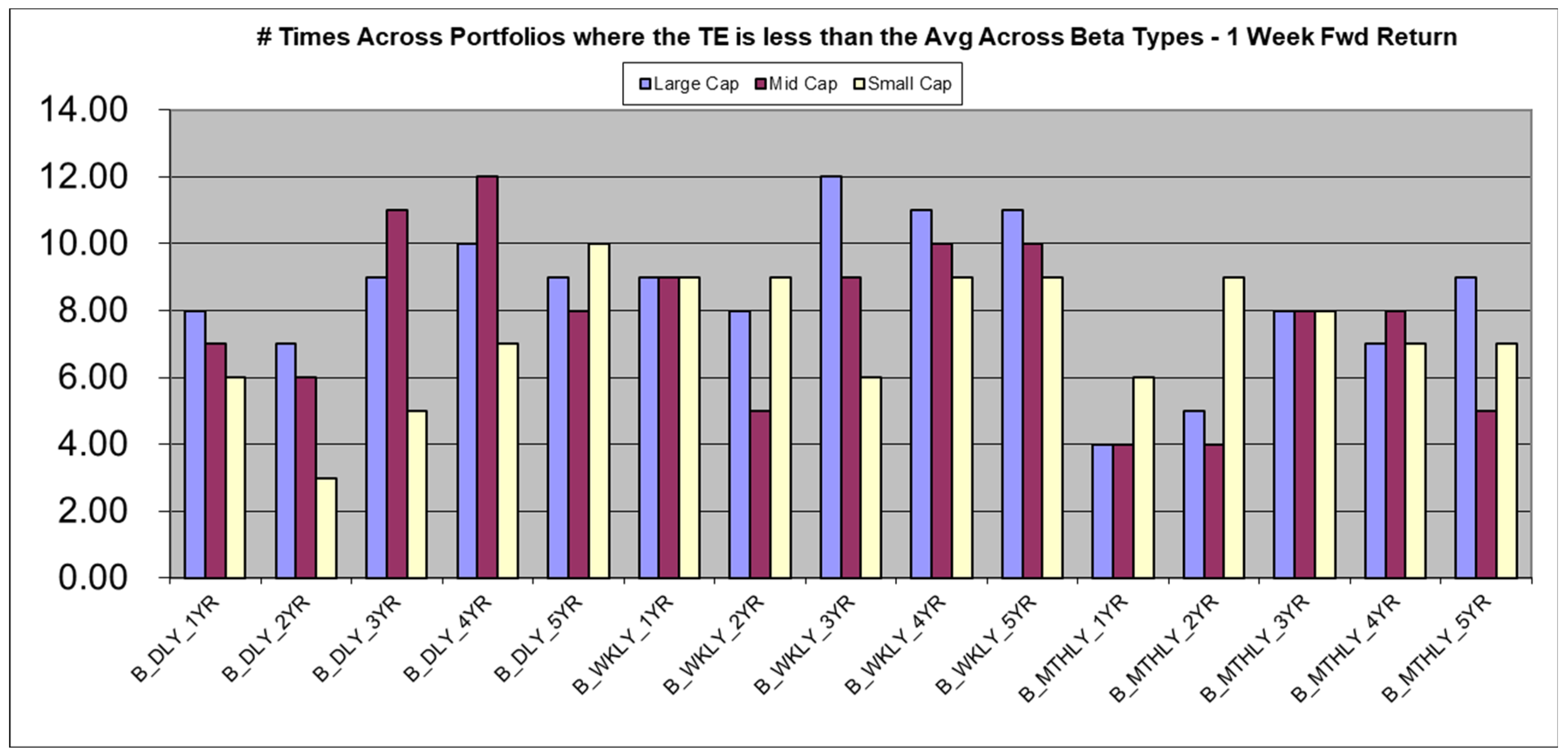
5
TE is the standard deviation of the difference between the realized and CAPM based forecast return vector.
6
We are operating within the Russell 1000 universe in a long time series dimension, hence three fractiles for Large, Mid and Small capitalization groups are formed.
7
p-value < 0.10 for all cells in Table 1 (A, B, C)
8
Across Row 1, in the 3 × 3 Classification matrix.

References

  1. Abate, Guido, Tommaso Bonafini, and Pierpaolo Ferrari. 2022. Portfolio Constraints: An Empirical Analysis. International Journal of Financial Studies 10: 9. [Google Scholar] [CrossRef]
  2. Agrrawal, Pankaj. 2009. An automation algorithm for harvesting capital market information from the web. Managerial Finance 35: 427–38. [Google Scholar] [CrossRef] [Green Version]
  3. Agrrawal, Pankaj. 2013. Using Index ETFs for Multi-Asset-Class Investing: Shifting the Efficient Frontier Up. The Journal of Index Investing 4: 83–94. [Google Scholar] [CrossRef]
  4. Agrrawal, Pankaj, John M. Clark, Rajat Agarwal, and Jivendra K. Kale. 2014. An Intertemporal Study of ETF Liquidity and Underlying Factor Transition, 2009–14. The Journal of Trading 9: 69–78. [Google Scholar] [CrossRef]
  5. Akono, Henri, Khondkar Karim, and Emeka Nwaeze. 2019. Analyst rounding of EPS forecasts and stock recommendations. Advances in Accounting 44: 68–80. [Google Scholar] [CrossRef]
  6. Alexeev, Vitali, Mardi Dungey, and Wenying Yao. 2016. Continuous and jump betas: Implications for portfolio diversification. Econometrics 4: 27. [Google Scholar] [CrossRef] [Green Version]
  7. Armitage, Seth, and Janusz Brzeszczynski. 2011. Heteroscedasticity and interval effects in estimating beta: UK evidence. Applied Financial Economics 21: 1525–38. [Google Scholar] [CrossRef]
  8. Black, Fischer. 1972. Capital market equilibrium with restricted borrowing. Journal of Business 45: 444–55. [Google Scholar] [CrossRef] [Green Version]
  9. Buckle, David. 2022. The Impact of Options on Investment Portfolios in the Short-Run and the Long-Run, with a Focus on Downside Protection and Call Overwriting. Mathematics 10: 1563. [Google Scholar] [CrossRef]
  10. Carhart, Mark M. 1997. On Persistence in Mutual Fund Performance. The Journal of Finance 52: 57–82. [Google Scholar] [CrossRef]
  11. Carroll, Carolyn, and KC John Wei. 1988. Risk, Return, and Equilibrium: An Extension. The Journal of Business 61: 485. [Google Scholar] [CrossRef]
  12. Chen, Nai-Fu, Richard Roll, and Stephen A. Ross. 1986. Economic Forces and the Stock Market. Journal of Business 59: 383. [Google Scholar] [CrossRef] [Green Version]
  13. Chu, Patrick, and Dan Xu. 2021. Tracking Errors and Their Determinants. Journal of Prediction Markets 1: 1851–65. [Google Scholar] [CrossRef]
  14. Chong, James. 2022. A trading strategy with dual-beta estimates. Managerial Finance 48: 720–32. [Google Scholar] [CrossRef]
  15. Cohen, Kalman J., Gabriel A. Hawawini, Steven F. Maier, Robert A. Schwartz, and David K. Whitcomb. 1983a. Estimating and Adjusting for the Intervalling-Effect in Beta. Management Science 29: 135. [Google Scholar] [CrossRef]
  16. Cohen, Kalman J., Gabriel A. Hawawini, Steven F. Maier, Robert A. Schwartz, and David K. Whitcomb. 1983b. Friction in the Trading Process and the Estimation of Systematic Risk. Journal of Financial Economics 12: 263. [Google Scholar] [CrossRef]
  17. Cooper, Ian. 2009. On Tests of the Conditional Relationship between Beta and Returns. Applied Financial Economics 19: 155–78. [Google Scholar] [CrossRef]
  18. Corhay, Albert. 1992. The Intervalling Effect Bias in Beta: A Note. Journal of Banking & Finance 16: 61. [Google Scholar]
  19. Corhay, Albert, and Alireza Tourani Rad. 1993. Return Interval, Firm Size and Systematic Risk on the Dutch Stock Market. Review of Financial Economics 2: 19. [Google Scholar] [CrossRef]
  20. Cremers, KJ Martijn, and Antti Petajisto. 2009. How Active is Your Fund Manager? A New Measure that Predicts Performance. The Review of Financial Studies 22: 3329–65. [Google Scholar] [CrossRef]
  21. CRSP via WRDS. 2022. Calculated (or Derived) Based on Data from Database Name ©2022 Center for Research in Security Prices (CRSP), The University of Chicago Booth School of Business and the Wharton Research Database Services. Available online: https://wrds-www.wharton.upenn.edu/ (accessed on 1 March 2022).
  22. Eichengreen, Barry. 2021. Bretton Woods After 50. Review of Political Economy 33: 552–69. [Google Scholar] [CrossRef]
  23. Fama, Eugene F., and Kenneth R. French. 1992. The Cross-Section of Expected Stock Returns. Journal of Finance 47: 427. [Google Scholar] [CrossRef]
  24. Fang, Yan, Florian Ielpo, and Benoît Sévi. 2012. Empirical Bias in Intraday Volatility Measures. Finance Research Letters 9: 231–37. [Google Scholar] [CrossRef]
  25. Fung, William KH, Robert A. Schwartz, and David K. Whitcomb. 1985. Adjusting for the Intervalling Effect Bias in Beta: A Test Using Paris Bourse Data. Journal of Banking & Finance 9: 443. [Google Scholar]
  26. Girard, Eric, and Amit K. Sinha. 2006. Does Total Risk Matter? The Case of Emerging Markets. Multinational Finance Journal 10: 117–51. [Google Scholar] [CrossRef]
  27. Goldsticker, Ralph, and Pankaj Agrrawal. 1999. The Effects of Blending Primary and Diluted EPS Data. Financial Analysts Journal 55: 51–60. [Google Scholar] [CrossRef] [Green Version]
  28. Graham, John R., and Campbell R. Harvey. 2001. The Theory and Practice of Corporate Finance: Evidence from the Field. Journal of Financial Economics 60: 187. [Google Scholar] [CrossRef]
  29. Groenewold, Nicolaas, and Patricia Fraser. 2000. Forecasting Beta: How well does the ‘Five-Year Rule of Thumb’ do? Journal of Business Finance & Accounting 27: 953. [Google Scholar]
  30. Hawawini, Gabriel A. 1980. An Analytical Examination of the Intervalling Effect on Skewness and Other Moments. Journal of Financial and Quantitative Analysis 15: 1121. [Google Scholar] [CrossRef]
  31. Hawawini, Gabriel A., and Ashok Vora. 1980. Evidence of Intertemporal Systematic Risks in the Daily Price Movements of NYSE and AMEX Common Stocks. Journal of Financial and Quantitative Analysis 15: 331. [Google Scholar] [CrossRef]
  32. Ho, Li-Chin Jennifer, and Jeffrey J. Tsay. 2001. Option Trading and the Intervalling Effect Bias in Beta. Review of Quantitative Finance and Accounting 17: 267. [Google Scholar] [CrossRef]
  33. Hollstein, Fabian, Marcel Prokopczuk, and Chardin Wese Simen. 2020. The Conditional Capital Asset Pricing Model Revisited: Evidence from High-Frequency Betas. Management Science 66: 2474–94. [Google Scholar] [CrossRef] [Green Version]
  34. Jarque, Carlos M., and Anil K. Bera. 1980. Efficient tests for normality, homoscedasticity and serial independence of regression residuals. Economics Letters 6: 255–59. [Google Scholar] [CrossRef]
  35. Jurdi, Doureige J., and Sam M. AlGhnaimat. 2021. The effects of ERM adoption on European insurance firms performance and risks. Journal of Risk and Financial Management 14: 554. [Google Scholar] [CrossRef]
  36. Lakonishok, Josef, and Alan C. Shapiro. 1986. Systematic Risk, Total Risk and Size as Determinants of Stock Market Returns. Journal of Banking & Finance 10: 115. [Google Scholar]
  37. Lei, Nuoa, Eric Masanet, and Jonathan Koomey. 2021. Best practices for analyzing the direct energy use of blockchain technology systems: Review and policy recommendations. Energy Policy 156: 112422. [Google Scholar] [CrossRef]
  38. Levene, Howard. 1960. Robust tests for equality of variances. In Ingram Olkin and Harold Hotelling: Contributions to Probability and Statistics: Essays in Honor of Harold Hotelling. Palo Alto: Stanford Press. [Google Scholar]
  39. Lin, Qi. 2021. The q5 model and its consistency with the intertemporal CAPM. Journal of Banking and Finance 127: 106096. [Google Scholar] [CrossRef]
  40. Lintner, John. 1965. The valuation of risk assets and the selection of risky investments in stock portfolios and capital budgets. Review of Economics and Statistics 47: 13–37. [Google Scholar] [CrossRef]
  41. Levy, Haim, Ilan Guttman, and Isabel Tkatch. 2001. Regression, Correlation, and the Time Interval: Additive-Multiplicative Framework. Management Science 47: 1150. [Google Scholar] [CrossRef] [Green Version]
  42. Mantsios, Georgios, and Stylianos Xanthopoulos. 2016. The Beta intervalling effect during a deep economic crisis: Evidence from Greece. International Journal of Business and Economic Sciences Applied Research 9: 19–26. [Google Scholar]
  43. Milonas, Nikolaos T., and Gerasimos G. Rompotis. 2013. Does intervalling effect affect ETFs? Managerial Finance 39: 863–82. [Google Scholar] [CrossRef]
  44. Pettengill, Glenn, Sridhar Sundaram, and Ike Mathur. 1995. The Conditional Relation between Beta and Returns. Journal of Financial and Quantitative Analysis 30: 101–16. [Google Scholar] [CrossRef] [Green Version]
  45. Reilly, Frank K., and David J. Wright. 1988. A Comparison of Published Betas. Journal of Portfolio Management 14: 64. [Google Scholar] [CrossRef]
  46. Roman, Mestre, and Michel Terraza. 2018. Time-Frequency varying beta estimation—A continuous wavelets approach. Economics Bulletin 38: 1796–810. [Google Scholar]
  47. Sharpe, William F. 1964. Capital asset prices: A theory of market equilibrium under conditions of risk. Journal of Finance 19: 425–42. [Google Scholar]
  48. Smith, Keith V. 1978. The Effect of Intervalling on Estimating Parameters of the Capital Asset Pricing Model. Journal of Financial and Quantitative Analysis 13: 313. [Google Scholar] [CrossRef]
  49. Terraza, Michel, and Mestre Roman. 2021. Adjusted beta based on an empirical comparison of OLS-CAPM and the CAPM with EGARCH errors. International Journal of Finance and Economics 26: 3588–98. [Google Scholar] [CrossRef]
  50. Verhoeven, Peter, Florian Sinn, and Tino T. Herden. 2018. Examples from Blockchain Implementations in Logistics and Supply Chain Management: Exploring the Mindful Use of a New Technology. Logistics 2: 20. [Google Scholar] [CrossRef]
  51. WRDS. 2022. Pricing Data on Stocks. Wharton Research Data Services. Available online: https://wrds-www.wharton.upenn.edu/ (accessed on 1 March 2022).
Figure 1. Scatterplot (3-D) of betas derived from daily, weekly and monthly returns (2000–2021).
Jrfm 15 00520 g001
Figure 2. Surface plot of betas derived from daily, weekly and monthly returns (2000−2021).
Jrfm 15 00520 g002
Figure 3. Weekly and daily betas have tracking errors mostly lower than monthly betas.
Jrfm 15 00520 g003
Table 1. Annualized Tracking Error of Actual Portfolio Return vs Beta Estimated Portfolio Return—All Periods.
A. Prediction of 1 Day Forward Return
Interval PeriodEstimation WindowLarge CapMid CapSmall CapLarge Cap/High BetaLarge Cap/Mid BetaLarge Cap/Low BetaMid Cap/High BetaMid Cap/Mid BetaMid Cap/Low BetaSmall Cap/High BetaSmall Cap/Mid BetaSmall Cap/Low Beta
Daily1 Year2.686.649.5011.344.806.4713.876.936.4317.679.746.93
2 Years2.586.258.9710.055.337.0612.906.806.8516.678.897.24
3 Years2.616.038.548.875.516.9111.876.936.7215.638.886.94
4 Years2.645.898.438.365.606.8611.257.076.7615.148.787.27
5 Years2.625.828.197.885.796.8310.487.106.7714.498.787.34
Weekly1 Year2.746.889.749.753.866.7213.807.006.9117.619.977.58
2 Years2.616.329.099.424.976.7612.696.956.4616.989.207.16
3 Years2.686.078.678.355.256.9612.086.846.7615.808.997.34
4 Years2.725.938.617.955.296.9311.487.166.6015.168.947.48
5 Years2.715.898.377.445.286.8011.137.106.5614.278.987.43
Monthly1 Year3.267.7812.5812.753.8410.7619.207.4611.5427.2611.5510.65
2 Years3.076.7710.5611.125.259.7815.997.259.0422.5110.259.06
3 Years3.156.409.599.665.519.3114.117.388.6819.529.548.36
4 Years3.026.199.369.135.728.6812.677.358.1117.599.668.33
5 Years2.896.108.848.625.728.1211.667.327.8216.229.128.21
Average2.806.339.279.385.187.6613.017.117.4717.509.427.82
B. Prediction of 1 Week Forward Return
Interval PeriodEstimation WindowLarge CapMid CapSmall CapLarge Cap/High BetaLarge Cap/Mid BetaLarge Cap/Low BetaMid Cap/High BetaMid Cap/Mid BetaMid Cap/Low BetaSmall Cap/High BetaSmall Cap/Mid BetaSmall Cap/Low Beta
Daily1 Year2.776.189.959.165.037.5712.526.937.3417.7910.447.65
2 Years2.766.239.798.425.187.6311.897.027.9817.309.927.75
3 Years2.876.119.628.155.507.7111.276.717.6316.989.827.87
4 Years2.906.049.428.005.627.5610.677.007.8016.369.957.89
5 Years2.966.129.207.645.757.6310.457.018.1015.979.907.79
Weekly1 Year2.755.949.468.684.477.5612.156.547.0716.739.737.98
2 Years2.835.929.388.755.287.5711.577.227.4116.679.557.39
3 Years2.985.809.198.225.607.7511.097.017.4816.349.267.55
4 Years3.015.758.967.975.617.8310.597.107.4215.789.437.60
5 Years3.075.858.757.855.707.9810.337.617.4715.149.377.59
Monthly1 Year3.096.119.6110.064.6210.2314.606.5310.7520.648.9511.73
2 Years3.196.159.178.674.679.0912.416.899.3617.349.209.17
3 Years3.275.958.977.824.978.5411.167.098.3115.929.318.70
4 Years3.245.938.807.595.388.1710.567.108.2015.599.098.41
5 Years3.256.018.627.495.697.9610.307.298.0215.079.378.09
Average3.006.019.268.305.278.0511.447.008.0216.649.558.21
C. Prediction of 1 Month Forward Return
Interval PeriodEstimation WindowLarge CapMid CapSmall CapLarge Cap/High BetaLarge Cap/Mid BetaLarge Cap/Low BetaMid Cap/High BetaMid Cap/Mid BetaMid Cap/Low BetaSmall Cap/High BetaSmall Cap/Mid BetaSmall Cap/Low Beta
Daily1 Year2.936.4010.5810.195.157.2311.417.978.4318.4111.349.35
2 Years3.016.6210.278.765.407.8211.298.268.8517.7310.979.36
3 Years3.036.6710.288.255.577.8911.008.158.6817.0811.149.30
4 Years3.056.7010.137.895.727.9610.768.358.6116.6810.969.30
5 Years3.156.7010.047.275.918.1110.468.458.6116.3711.099.30
Weekly1 Year3.006.0610.039.204.377.1110.527.637.8517.2110.459.19
2 Years3.076.329.789.364.957.5210.867.978.1016.7110.248.69
3 Years3.136.419.778.485.457.5510.527.988.2416.1310.648.77
4 Years3.166.459.638.325.477.6510.458.138.1915.8510.578.79
5 Years3.276.499.587.735.747.7610.258.388.2915.6110.708.86
Monthly1 Year3.136.3910.3610.754.558.9514.007.1611.0620.2210.6012.42
2 Years3.366.469.718.745.048.1111.867.808.9217.3610.669.57
3 Years3.416.559.667.915.397.9810.788.168.6515.5110.899.04
4 Years3.386.599.537.715.447.5710.407.908.3115.3310.338.95
5 Years3.446.639.517.365.737.5410.178.208.1515.0210.398.99
Average3.176.509.928.535.337.7810.988.038.6016.7510.739.33
Green-Daily Beta with lowest TE; Red-Weekly Beta with lowest TE; Yellow-Month Beta with lowest TE; p-value < 0.10 for all cells.
Table 2. 3 × 3 Classification Matrix of ’Minimum’ Tracking Errors.
Interval Length
Forecast Length
Daily BetasWeekly BetasMonthly BetasTotal TE’s%Best
1 Day9, a1211275.0%, a1
1 Week06, b261250.0%, b2
1 Month264, c31233.3%, c3
Table 3. Tests for equality of means and variance homogeneity (daily, weekly and monthly betas).
Test for equal means
Sum of SquaresdfMean squareFp (same)
Between Beta groups:1.731920.86604.57200.010420
Within Beta groups:543.835028710.1894Permutation p (n = 99,999)
Total:545.567028730.0105
Kruskal-Wallis test for equal medians H (chi2):6.327
(non-parametric test) p (same):0.04227
There is a significant difference betweenthe sample means and also the medians
Levene’s test for homogeneity of variance p (same):4.94 × 10⁻²⁷
Welch F test for unequal variances: F = 5.734, df = 1857, p = 0.003293
All p-values indicate that the Betas for Daily, Weekly and Monthly intervals differ in means, medians and variance.
Publisher’s Note: MDPI stays neutral with regard to jurisdictional claims in published maps and institutional affiliations.

