Article

Pricing European Options under Stochastic Volatility Models: Case of Five-Parameter Variance-Gamma Process

by
Aubain Hilaire Nzokem
Department of Mathematics & Statistics, University of Massachusetts Amherst, Amherst, MA 01003, USA
J. Risk Financial Manag. 2023, 16(1), 55; https://doi.org/10.3390/jrfm16010055
Submission received: 5 December 2022 / Revised: 8 January 2023 / Accepted: 12 January 2023 / Published: 16 January 2023
(This article belongs to the Special Issue Mathematical and Empirical Finance)

Abstract

:
The paper builds a Variance-Gamma (VG) model with five parameters: location ( μ ), symmetry ( δ ), volatility ( σ ), shape ( α ), and scale ( θ ); and studies its application to the pricing of European options. The results of our analysis show that the five-parameter VG model is a stochastic volatility model with a Γ ( α , θ ) Ornstein–Uhlenbeck type process; the associated Lévy density of the VG model is a KoBoL family of order ν = 0 , intensity α , and steepness parameters δ σ 2 δ 2 σ 4 + 2 θ σ 2 and δ σ 2 + δ 2 σ 4 + 2 θ σ 2 ; and the VG process converges asymptotically in distribution to a Lévy process driven by a normal distribution with mean ( μ + α θ δ ) and variance α ( θ 2 δ 2 + σ 2 θ ) . The data used for empirical analysis were obtained by fitting the five-parameter Variance-Gamma (VG) model to the underlying distribution of the daily SPY ETF data. Regarding the application of the five-parameter VG model, the twelve-point rule Composite Newton–Cotes Quadrature and Fractional Fast Fourier (FRFT) algorithms were implemented to compute the European option price. Compared to the Black–Scholes (BS) model, empirical evidence shows that the VG option price is underpriced for out-of-the-money (OTM) options and overpriced for in-the-money (ITM) options. Both models produce almost the same option pricing results for deep out-of-the-money (OTM) and deep-in-the-money (ITM) options.

1. Introduction

The Black–Scholes (BS) model Black and Scholes (1973) is considered the cornerstone of option pricing theory. The model relies on the fundamental assumption that asset returns have a normal distribution with a known mean and variance. However, based on empirical studies, the Black–Scholes (BS) model is inconsistent with a set of well-established stylized features Cont (2001). Due to the subsequent development of option pricing theory, a new class of models has emerged in the literature to address the stylized characteristics of the markets. The probabilistic property of infinitely divisible distribution is the main characteristic of these new models, which belong to the family of Lévy processes Kyprianou (2014).
The new class of models can be divided into two subclasses: Jump-Diffusion and Stochastic Volatility. The Jump-Diffusion process is modeled as an independent Brownian motion plus a Compound Poisson Process. The popular models in the literature are Merton’s jump-diffusion model Matsuda (2004) and Kou’s jump-diffusion model Kou (2002), in which the logarithmic jump size follows a normal distribution and an asymmetric double exponential distribution, respectively. Stochastic volatility (SV) models are another extension of the standard geometric Brownian motion (GBM) model, where the observed volatility is modeled as a stochastic process. In a stochastic volatility framework Alhagyan et al. (2020), the constant volatility ( σ ) in a standard geometric Brownian motion model is replaced by a deterministic function of a stochastic process ( σ ( Y t ) ), where Y t represents the solution of the stochastic differential equation (SDE). There are two main types of SV models in the literature: diffusion-based SV models and non-Gaussian Ornstein–Uhlenbeck based SV models. In the popular diffusion-based SV models, Y t follows a Cox-Ingersoll-Ross (CIR) process Heston (1993) or a Log-normal process Hull and White (1987). The deterministic function is a squared root of the stochastic process ( σ ( Y t ) = Y t ). The non-Gaussian Ornstein–Uhlenbeck based SV models were introduced and thoroughly studied in Barndorff-Nielsen et al. (1998) and Barndorff-Nielsen and Shephard (2001b, 2002, 2003). The SV model with the Ornstein–Uhlenbeck type process is mathematically tractable and has many appealing features.
From the perspective of derivative asset analysis, we will build a five-parameter VG model as a stochastic volatility model with a Γ ( α , θ ) Ornstein–Uhlenbeck type process. While there are a large number of studies on option pricing using the VG model, most of the papers in the literature use three parameters Adeosun et al. (2016); Li et al. (2020); Madan et al. (1998); Mozumder et al. (2015), which is certainly due to technical issues inherent in fitting a high-parametric model to the marginal distribution of asset returns. The number of studies in the literature considering a VG model with five parameters is rather limited. Using the five-parameter Variance-Gamma model as an underlying distribution of European options allows us to control both the excess kurtosis and the skewness in the market data. In option pricing theory, the main challenge often involves the existence of the Equivalent Martingale Measure (EMM) and whether it preserves the structure of the Variance-Gamma measure. The Variance-Gamma (VG) process is not a Gaussian process, and the market is incomplete; therefore, the Equivalent Martingale Measure is not unique. The Esscher transform of the historical measure is considered optimal with respect to some optimization criterion Boyarchenko and Levendorskii (2002). The Esscher Martingale measure was shown in Andrusiv and Engelbert (2020) to coincide with the minimal entropy Martingale measure for Lévy processes.
The remainder of the paper is organized as follows. Section 2 is devoted to building a five-parameter VG process, presenting parameter estimations and simulations of the VG process. Section 3 investigates the Lévy density and asymptotic distribution of the VG process. Finally, in Section 4, we extend the Black–Scholes framework, provide the integral representation for the option price, and compute the VG option price numerically.

2. Variance-Gamma Process: Stochastic Volatility Model

2.1. Lévy Framework and Asset Pricing

Let ( Ω , F , F t t 0 , P ) be a filtered probability space, with F = t > 0 F t , F t t 0 a filtration, F t a σ -algebra included in F , and F τ F t for τ < t .
A stochastic process Y = { Y t } t 0 is a Lévy process if it has the following properties:
(L1): Y 0 = 0 a.s.
(L2): Y t has independent increments, that is, for 0 < t 1 < t 2 < < t n , the random variables Y t 1 , Y t 1 Y t 2 , …, Y t n Y t n 1 are independent
(L3): Y t has stationary increments, that is, for any t 1 < t 2 < + the probability distribution of Y t 1 Y t 2 depends only on t 1 t 2
(L4): Y t is stochastically continuous; for any t and ϵ > 0 , lim s t P | Y s Y t | > ϵ = 0
(L5): c à d l à g paths, that is, t Y t is a.s. right continuous with left limits
Given a Lévy process Y = { Y t } t 0 on the filtered probability space ( Ω , F , F t t 0 , P ) , we define the asset value process S = { S t } t 0 such as S t = S 0 e Y t .
Theorem 1.
(Lévy–Khintchine representation)
Let Y = { Y t } t 0 be a Lévy process on R . Then, the characteristic exponent admits the following representation:
φ ( ξ ) = L o g E e i Y 1 ξ = i γ ξ + 1 2 σ 2 ξ 2 + 0 t e i ξ y 1 y ξ 1 | y | 1 Π ( d y )
where γ R , σ 0 , and Π is a σ-finite measure called the Lévy measure of Y, satisfying the property
+ M i n ( 1 , | y | 2 ) Π ( d y ) < +
For the theorem-proof, see Applebaum (2009); Ken-Iti (1999); Tankov (2003).
Each Lévy process is uniquely determined by the Lévy–Khintchine triplet ( γ , σ 2 , Π ) . The terms of this triplet suggest that a Lévy process can be seen as having three independent components: a linear drift, a Brownian motion, and a Lévy jump process. With the diffusion term σ = 0 , we have a Lévy jump process; in addition, if γ = 0 , we have a pure jump process.

2.2. Γ ( α , θ ) Ornstein–Uhlenbeck Proces

The Ornstein–Uhlenbeck process is a diffusion process introduced by Ornstein and Uhlenbeck Uhlenback and Ornstein (1930) to model the stochastic behavior of the velocity of a particle undergoing Brownian motion. Ornstein–Uhlenbeck diffusion σ 2 = { σ 2 ( t ) , t 0 } is the solution of the Langevin Stochastic Differential Equation (SDE) (2)
d σ 2 ( t ) = λ σ 2 ( t ) d t + d B ( λ t ) .
where λ > 0 and B = { B t , t 0 } is a Brownian motion.
In recent years, the Ornstein–Uhlenbeck process has been used in finance to capture important distributional deviations from Gaussianity and to model dependence structures. The extension of the Ornstein–Uhlenbeck process has been obtained by replacing the Brownian motion in (2) by z(t), which is a background driving Lévy process (BDLP) Barndorff-Nielsen and Shephard (2001a, 2002, 2003). The SDE (2) becomes
d σ 2 ( t ) = λ σ 2 ( t ) d t + d z ( λ t ) λ > 0 .
where the process z ( t ) = { z ( t ) , t 0 , z ( 0 ) = 0 } is subordinator, that is, a process with non-negative, independent, and stationary increments, which implies σ 2 ( t ) 0 . Correspondingly, z(t) moves up entirely by jumps and then tails off exponentially Barndorff-Nielsen and Shephard (2001b).
Lemma 1.
The general form of the stationary process σ 2 ( t ) , a solution of (3), is provided by
σ 2 ( t ) = 0 + e s d z ( λ t s ) λ > 0 .
Proof. 
σ 2 ( t ) = 0 + e s d z ( λ t s ) = 0 + e λ s d z ( λ ( t s ) ) = t e λ ( t s ) d z ( λ s )
By using the variable changing method, we can have different expressions of (4).
σ 2 ( t ) = t e λ ( t s ) d z ( λ s ) d σ 2 ( t ) = λ σ 2 ( t ) d t + d z ( λ t )
Expression (5) can be written as follows:
σ 2 ( t ) = e λ t σ 2 ( 0 ) + 0 t e λ ( t s ) d z ( λ s ) σ 2 ( 0 ) = 0 e λ s d z ( λ s )
Theorem 2.
Assume that z ( t ) = k = 1 N ( t ) ξ k is a compound poison process, that is, N(t) is a Poisson process with instantaneous rate α and ξ k follows an exponential distribution with rate θ.
The stationary marginal distribution of σ 2 ( t ) is the Gamma distribution Γ ( α , θ )
Proof. 
σ 2 ( t + u ) = t + u e λ ( t + u s ) d z ( λ s ) = e λ u σ 2 ( t ) + 0 u e λ ( u s ) d z ( λ s ) u 0
The stationary solution σ 2 ( t ) of (3) can be written as in (8). Because of the stationarity, we have
ϑ ( ξ ) = ϑ ( ξ e λ u ) Φ ( u , ξ )
where ϑ ( ξ ) is the characteristic function of the stationary distribution of σ 2 ( t ) and Φ ( u , ξ ) is the characteristic function of 0 u e λ ( u s ) d z ( λ s ) . We have 0 e λ u 1 for u 0 , and the relation (8) shows that σ 2 ( t ) is self-decomposable.
z ( t ) is a compound Poisson process with the following characteristic function:
g ( ξ ) = E ( e i ξ z ( 1 ) ) = e x p 0 ( e i ξ x 1 ) α f ( x ) d x = e x p ( ρ ( ξ ) ) ρ ( ξ ) = i ξ α θ i ξ
It was shown in Barndorff-Nielsen et al. (1998) that Φ ( u , ξ ) can be expressed as follows:
Φ ( u , ξ ) = e x p λ 0 u ρ ( ξ e λ ( u s ) ) d s = e x p ξ e λ u ξ ρ ( w ) w d w
By replacing, ρ ( w ) w = i α θ i w , we have
Φ ( u , ξ ) = θ i ξ e λ u θ i ξ α
where ϑ ( ξ ) is continuous at zero, and we have
ϑ ( ξ ) = lim u ϑ ( ξ e λ u ) Φ ( u , ξ ) = 1 1 i 1 θ ξ α = 1 i θ 1 ξ α
From (13), ϑ ( ξ ) is the characteristic function of the gamma distribution, and the stationary marginal distribution of σ 2 ( t ) is the Gamma distribution Γ ( α , θ ) .
Another method developed in Barndorff-Nielsen and Shephard ( 2001a, 2001b, 2002, 2003) uses the relationship between the z ( t ) Lévy density w ( x ) and the Lévy density u ( x ) of σ 2 ( t ) :
u ( x ) = 1 w ( x r ) d r
From (10), we have the Lévy density w ( x ) = α f ( x ) = α θ e θ x , and the Lévy density u ( x ) of σ 2 ( t ) can be deduced as follows:
u ( x ) = 1 α θ e θ x r d r = α x e θ x x > 0
which is the Lévy density of the Gamma distribution Γ ( α , θ ) . □
We can integrate the stationary non-negative process σ 2 ( t ) as follows:
σ 2 * ( t ) = 0 t σ 2 ( s ) d s
By integration using part method, (16) becomes
σ 2 * ( t ) = λ 1 σ 2 ( 0 ) ( 1 e λ t ) + λ 1 0 t 1 e λ ( t s ) d z ( λ s )
= λ 1 σ 2 ( t ) + z ( λ t ) + σ 2 ( 0 )
It results from (18) that the process σ 2 * ( t ) is continuous, as z ( λ t ) and σ 2 ( t ) co-break Barndorff-Nielsen and Shephard (2001b, 2002). In addition, the shape of σ 2 * ( t ) is determined by z ( λ t ) . In fact, σ 2 * ( t ) and z ( λ t ) co-integrate. The co-integration can be shown by transforming Equation (18) into Equation (19). λ σ 2 * ( t ) z ( λ t ) is a stationary process such that
λ σ 2 * ( t ) z ( λ t ) = σ 2 ( t ) + σ 2 ( 0 ) .
For λ = 1 and σ 2 ( 0 ) = 0 , the compound Poisson process ( z ( t ) ), the Γ ( α , θ ) Ornstein–Uhlenbeck process in ( σ 2 ( t ) ), and σ 2 * ( t ) in (20) were simulated, with the results shown in Figure 1a, Figure 1b, and Figure 1c, respectively.
z ( t ) = k = 1 N ( t ) ξ k σ 2 ( t ) = σ 2 ( 0 ) e λ t + k = 1 N ( t ) e x p ( λ ( t a k ) ) ξ k σ 2 * ( t ) = 0 t σ 2 ( s ) d s
The estimations of the Gamma distribution parameter Γ ( α , θ ) were performed by applying the FRFT maximum likelihood to the daily SPY ETF prices Nzokem (2021a).

2.3. Variance-Gamma Process: Semi-Martingale

Let Y * = { Y t * } , a stochastic process used to model the log of an asset price.
Y t * = A t + M t A t = β t + δ σ 2 * ( t )
M t = σ 0 t σ ( s ) d W ( s )
where β and δ are the drift parameters, t represents the continuous time clock, and W ( t ) is the standard Brownian motion and is independent of σ 2 ( t ) .
σ ( t ) = σ 2 ( t ) σ 2 * ( t ) = 0 t σ 2 ( s ) d s
where σ ( t ) is the spot or instantaneous volatility and σ 2 * ( t ) is the chronometer or integrated variance of the process. As shown in Figure 1c, the Gamma process ( σ 2 * ( t ) ) is a strictly increasing process of the stationary process ( σ 2 ( t ) ).
The mean process A t is a predictable process with locally bounded variation. In fact, A t is continuous and differentiable because of σ 2 * ( t ) .
M t is a local Martingale. The derivative of M t in (22) can be written as a stochastic differential equation (SDE) (24):
d M t = σ σ ( t ) d W ( t )
where Y t * is a special semi-Martingale Barndorff-Nielsen and Shephard (2002); Protter (2005) and the decomposition Y t * = A t + M t is unique.
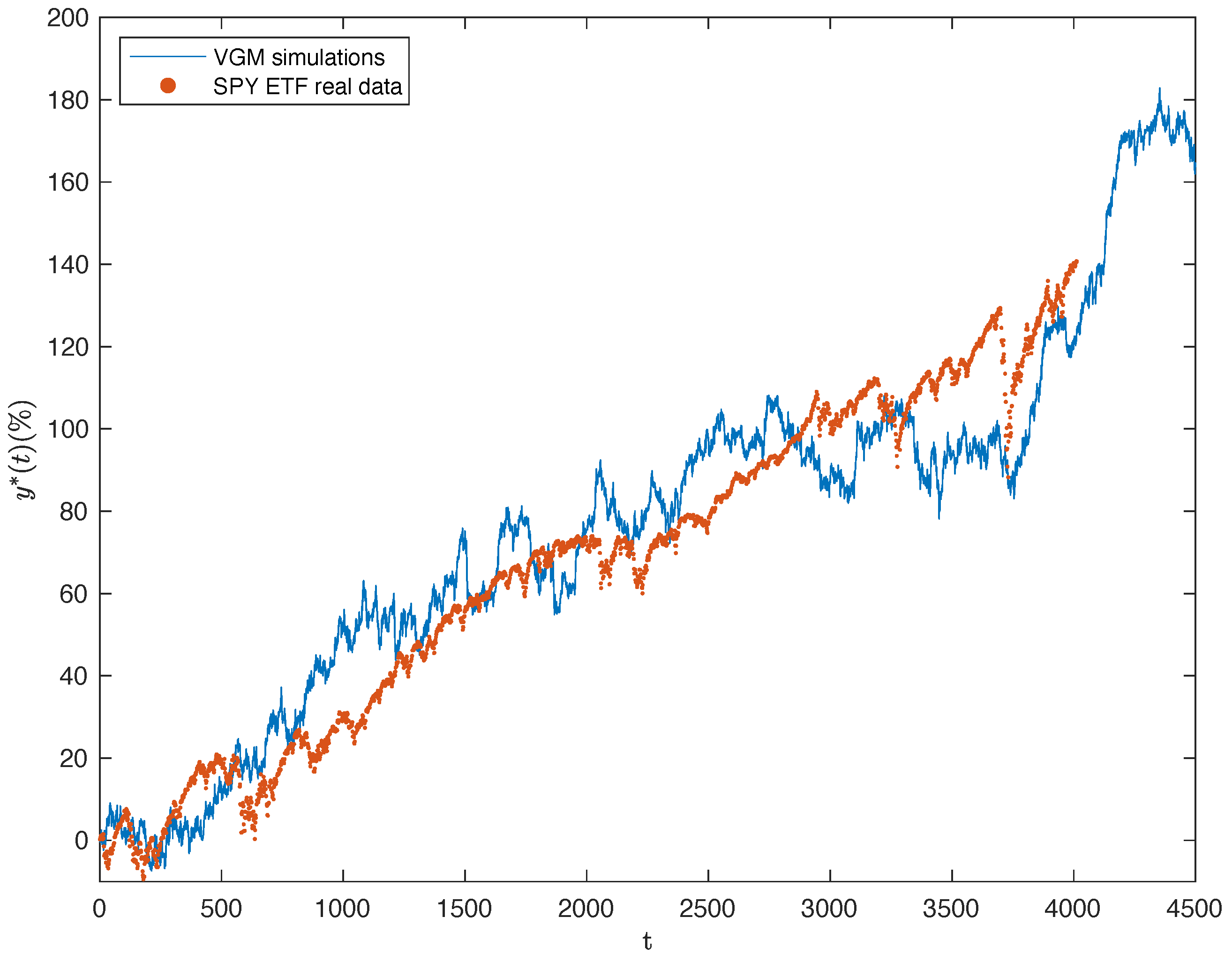
Figure 2, in blue, displays the simulation results for the logarithmic of the asset price ( Y * ) in (21). The simulation results are compared with the daily SPY ETF historical return data from 4 January 2010 to 30 December 2020, displayed in red.

2.4. Variance-Gamma Process: Parameter Estimations

The stochastic process in (21) is the solution of the following stochastic differential equation (SDE):
d Y t * = ( β + δ σ 2 ( t ) ) d t + σ σ ( t ) d W ( t )
Considering an interval of length Δ , we define σ n 2 and Y n over the interval [ ( n 1 ) Δ ; n Δ ].
σ n 2 = ( n 1 ) Δ n Δ d σ 2 * ( s ) = σ n Δ 2 * σ ( n 1 ) Δ 2 * Y n = ( n 1 ) Δ n Δ d Y s * = Y n Δ * Y ( n 1 ) Δ *
The volatility component can be transformed into a normally distributed variable X ( 1 ) as follows:
( n 1 ) Δ n Δ σ ( t ) d W ( t ) = d N 0 , ( n 1 ) Δ n Δ σ 2 ( s ) d s = N 0 , σ n Δ 2 * σ ( n 1 ) Δ 2 * = N 0 , σ n 2 = d σ n N 0 , 1 = d σ n X ( 1 ) .
where X ( 1 ) = d N ( 0 , 1 ) and N ( 0 , 1 ) denotes a standard normal distribution.
By integrating the instantaneous return rate (25) per component, we have
( n 1 ) Δ n Δ d Y s * = β Δ + δ ( n 1 ) Δ n Δ d σ 2 * ( s ) + σ ( n 1 ) Δ n Δ σ ( t ) d W ( t )
Based on (26) and (27), we have the following equation over the interval [ ( n 1 ) Δ ; n Δ ]:
Y n = μ + δ σ n 2 + σ σ n X ( 1 ) μ = β Δ σ n 2 = d Γ ( α , θ )
In the case where Δ is a daily length, Y n becomes the daily return rate. Equation (28) was analyzed in Nzokem (2021a, 2021b) as a daily return rate, and the parameters were estimated. The data came from the daily SPY ETF prices for the period spanning from 4 January 2010 to 30 December 2020; see Nzokem (2021a, 2021b, 2021d) for more details on the methodology and results.
Table 1 presents the estimation results of the five parameters ( μ , δ , α , θ , σ ) of Y n in (28) along with four statistical indicators.
As shown in Table 2, with initial parameter values ( σ = α = θ = 1 , δ = μ = 0 ), the maximization procedure convergences after 21 iterations. The values of the optimizing function ( log ( M L ) ) are provided along with the values of | | d log ( M L ) d V | | . During the maximization process, both quantities converge to 3549.692 and 0, respectively. The location parameter μ is positive, the symmetric parameter δ is negative, and other parameters have the expected sign.

3. Variance-Gamma Process: Probability versus Lévy Density

Based on (21) and (22), the VG Process Y = { Y t } t 0 with five parameters ( μ , δ , σ , α , θ ) can be written as follows:
Y t = μ t + δ σ 2 * ( t ) + σ 0 t σ ( s ) d W ( s ) .
where μ , δ R , σ > 0 , α > 0 , θ > 0 , t represents the continuous time clock, W ( t ) is the standard Brownian motion and is independent of σ 2 ( t ) , and
σ 2 * ( t ) = 0 t σ 2 ( s ) d s σ ( t ) = σ 2 ( t )
where σ ( t ) is the spot or instantaneous volatility, σ 2 ( t ) is the spot or instantaneous variance, and σ 2 * ( t ) is the chronometer or the integrated variance of the process.
We now consider the characteristic function of the VG process Y = { Y t } :
E e i ξ Y t = E e i ξ ( μ t + δ σ 2 * ( t ) + σ 0 t σ ( s ) d W ( s ) ) = e i t μ ξ E e i ξ ( δ σ 2 * ( t ) + σ 0 t σ ( s ) d W ( s ) ) .
where 0 t σ ( s ) d W ( s ) is the It o ^ integral with respect to the Brownian motion, and we have
0 t σ ( s ) d W ( s ) = d N 0 , 0 t σ 2 ( s ) d s = N 0 , σ 2 * ( t )
where N ( 0 , 1 ) is a standard normal distribution.
From expressions (31) and (32), we have
E e i ξ ( δ σ 2 * ( t ) + σ 0 t σ ( s ) d W ( s ) ) = E e i ξ N δ σ 2 * ( t ) , σ 2 σ 2 * ( t ) = E E e i ξ N δ σ 2 * ( t ) , σ 2 σ 2 * ( t ) | σ 2 * ( t ) = E e ( i δ ξ 1 2 σ 2 ξ 2 ) σ 2 * ( t )
where σ 2 * ( t ) is a Lévy process generated by the Gamma distribution Γ ( α , θ ) , and we have
E e ( i δ ξ 1 2 σ 2 ξ 2 ) σ 2 * ( t ) = 1 ( 1 + 1 2 θ σ 2 ξ 2 ) t α E e i δ ξ W σ 2 * ( t ) = d Γ ( t α , θ ) = 1 1 i δ θ ξ + 1 2 σ 2 θ ξ 2 t α W = d Γ ( t α , 1 2 σ 2 ξ 2 + 1 θ )
From expressions (31), (33), and (34), we have
E e i Y t ξ = e i t μ ξ 1 i δ θ ξ + 1 2 σ 2 θ ξ 2 t α
We define two related functions ϕ ( ξ ) and φ ( ξ , t ) such that
ϕ ( ξ ) = e i μ ξ 1 i δ θ ξ + 1 2 σ 2 θ ξ 2 α φ ( ξ , t ) = L o g ( E e i Y t ξ ) = t L o g ( ϕ ( ξ ) )
The characteristic function can be written as follows:
E e i Y t ξ = ϕ ( ξ ) t = E [ e t L o g ( ϕ ( ξ ) ) ]

3.1. Lévy Measure and the Structure of the Jumps

Lemma 2.
(Frullani integral) α , β > 0 and z C with ( z ) 0 .
We have
1 1 z α β = e 0 ( 1 e z x ) β x 1 e α x d x
For lemma proof, see Arias-de Reyna (1990).
Theorem 3.
(Variance-Gamma model representation)
Let Y = { Y t } t 0 , a Lévy process on R generated by the VG model with parameter ( μ , δ , σ , α , θ ) . The characteristic exponent of the Lévy process has the following representation:
φ ( ξ , 1 ) = L o g E e i Y 1 ξ = i μ ξ + + 1 e i ξ u Π ( u ) d u
Π ( u ) is the Lévy density of Y and has the following expression:
Π ( u ) = α 1 { u > 0 } u e x 1 u + 1 { u < 0 } | u | e x 2 u
with
x 1 = δ σ 2 + δ 2 σ 4 + 2 θ σ 2 x 2 = δ σ 2 δ 2 σ 4 + 2 θ σ 2
and Π ( u ) satisfies the following properties:
+ Π ( u ) d u = + a n d + M i n ( 1 , | u | ) Π ( u ) d u < +
Proof. 
We consider the characteristic function ϕ ( ξ ) in (36) of the VG model with parameter ( μ , δ , σ , α , θ ) , as developed previously:
ϕ ( ξ ) = e i μ ξ 1 i δ θ ξ + 1 2 σ 2 θ ξ 2 α
We factor the quadratic function in the denominator of ϕ ( ξ )
1 + 1 2 θ σ 2 x 2 i δ θ x α = 1 2 θ σ 2 α x i x 1 α x i x 2 α
with
x 1 = δ σ 2 + δ 2 σ 4 + 2 θ σ 2 x 2 = δ σ 2 δ 2 σ 4 + 2 θ σ 2
We apply Lemma 2 on each factor of the quadratic function (42):
1 2 θ σ 2 α x i x 1 α x i x 2 α = 1 + i x x 1 α 1 + i x x 2 α = e 0 ( 1 e i x u ) α u e x 1 u d u e 0 ( 1 e i x u ) α u e x 2 u d u = e 0 ( 1 e i x u ) α u e x 1 u d u + 0 ( 1 e i x v ) α | v | e x 2 v d v = e + ( 1 e i x u ) Π ( u ) d u
taking into account the expression (42), we have
1 + 1 2 θ σ 2 x 2 i δ θ x α = e + ( 1 e i x u ) Π ( u ) d u .
where Π ( u ) = α 1 { u > 0 } u e x 1 u + 1 { u < 0 } | u | e x 2 u
From expression (36), we have
φ ( ξ , t ) = t L o g ( ϕ ( ξ ) ) = i t μ ξ + t L o g 1 + 1 2 θ σ 2 x 2 i δ θ x α = i t μ ξ + t L o g 1 + 1 2 θ σ 2 x 2 i δ θ x α = i t μ ξ + + ( 1 e i x u ) t Π ( u ) d u
We have
φ ( ξ , t ) = t L o g ( ϕ ( ξ ) ) = i t μ ξ + + ( 1 e i x u ) t Π ( u ) d u
For t = 1 , we have the expression (38).
We can check the properties of Π ( u ) as follows:
+ Π ( u ) d u = + in fact lim | u | 0 Π ( u ) = +
+ M i n ( 1 , | u | ) Π ( d u ) = 1 1 M i n ( 1 , | u | ) Π ( d u ) + 1 + M i n ( 1 , | u | ) Π ( d u ) + 1 M i n ( 1 , | u | ) Π ( d u ) = α 1 e x 1 x 1 + 1 e x 2 x 2 + Γ ( 0 , x 1 ) + Γ ( 0 , x 2 ) .
with Γ ( s , u ) = u + y s 1 e y d y .
Finally, we have
+ M i n ( 1 , | u | ) Π ( d u ) < +
It results from (45) that the VG process is not a finite activities process and cannot be written as a compound Poisson process Barndorff-Nielsen and Shephard (2002). The VG process is an infinite activity process with an infinite number of jumps in any given time interval. The arrival rate of jumps of all sizes in the VG process is defined by the Lévy density (47):
Π ( u ) = α | u | e x 2 u if u < 0 α u e x 1 u if u > 0 .
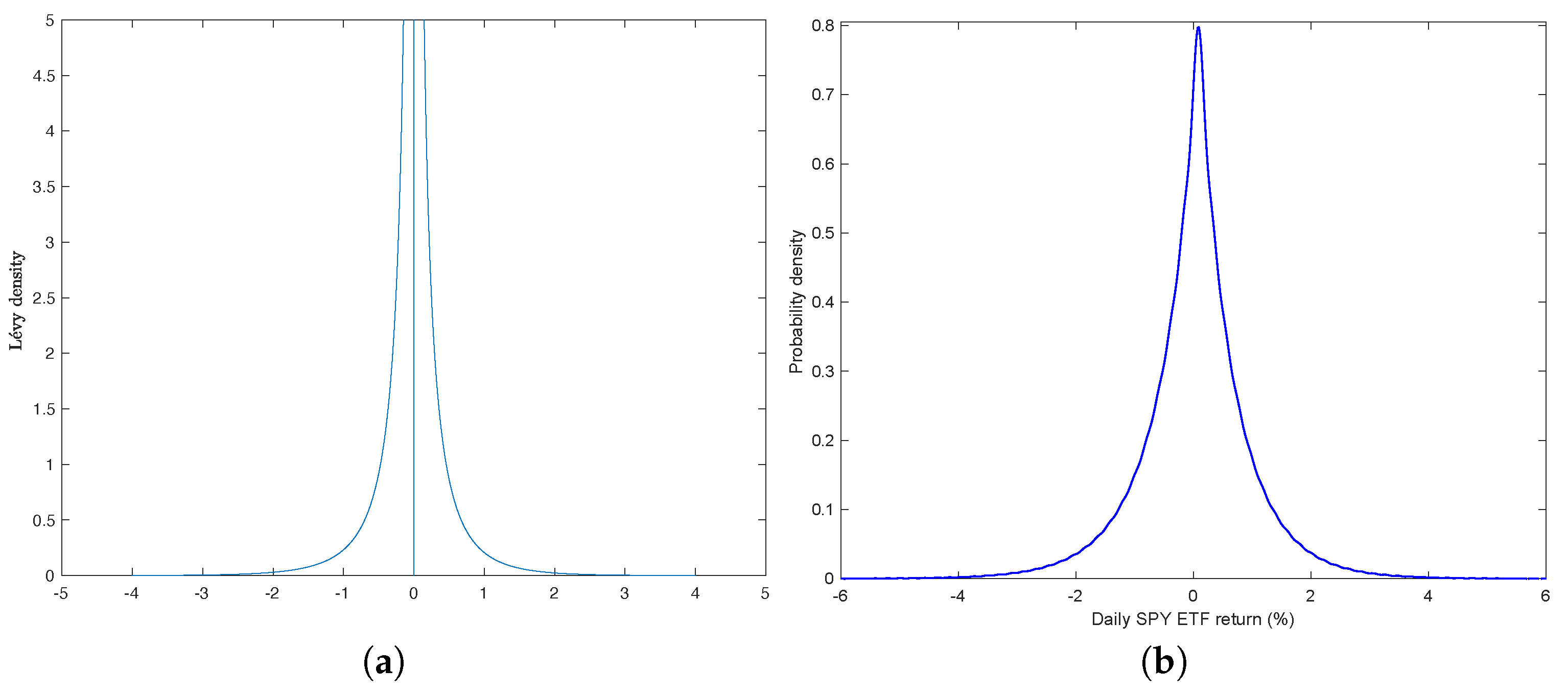
As shown in Figure 3a, the high arrival rates of jumps are concentrated around the origin 0. The smaller the jump size, the higher the arrival rate for the VG model. The steepness parameters Boyarchenko and Levendorskii (2002), x 2 and x 1 , define the rate of exponential decay of the tails on each side. As shown in Figure 3a and (47), the Lévy density is asymmetric, and the left tail is heavier as x 2 < x 1 . On the other hand, the result in (46) proves that the VG process is a finite variation process, which is contrary to the Brownian motion process. The Gamma distribution parameter ( α ), called the process intensity Boyarchenko and Levendorskii (2002), plays an important role in the Lévy density. The intensity of the process ( α ) has a similar role as the variance parameter in the Brownian motion process. The Lévy density function (47) is different for negative and positive jump sizes. This difference led Madan et al. (1998) to consider the VG process as the difference between two increasing processes, with one process providing the upward movement and another the downward movement in the market.
Using the VG parameter estimations in Table 1, we have x 1 = 1.4775 and x 2 = 1.3640 . The Lévy and probability densities are displayed in Figure 3a and Figure 3b, respectively. As shown in Figure 3, the shape of the density functions are different, even though the same characteristic function links both densities.
The Variance-Gamma (VG) process can be described as a subfamily of the KoBoL family, which is the extension of Koponen’s family by Boyarchenko and Levendorskii Boyarchenko and Levendorskii (2002). The KoBoL family is sometimes called the CGMY model (named after Carr, German, Madan, and Yor) Carr et al. (2003). Under the KoBoL family, the Lévy density has the following general form (see Boyarchenko and Levendorskii (2002) for more details):
Π ( u ) = C | u | ν 1 e λ u if u < 0 C + u ν 1 e λ + u if u > 0
where C + > 0 , C > 0 , ν > 0 , and λ < 0 < λ + .
As a subfamily of the KoBoL family, the VG process belongs to the process class with order ν = 0 , intensity C + = C = α , and steepness parameters λ = x 2 = δ σ 2 + δ 2 σ 4 + 2 θ σ 2 and λ + = x 1 = δ σ 2 + δ 2 σ 4 + 2 θ σ 2 . For 0 < ν < 1 , see Nzokem and Montshiwa (2022) for a general case of tempered stable distribution.

3.2. Variance-Gamma Process: Asymptotic Distribution

Theorem 4.
(Variance-Gamma process probability density)
Let Y = { Y t } t 0 , a Lévy process on R generated by the VG model with parameter ( μ , δ , σ , α , θ ) . The probability density function can be written as follows:
f ( y , t ) = 1 σ Γ ( t α ) θ t α 0 + 1 2 π v e ( y t μ δ v ) 2 2 v σ 2 v t α 1 e v θ d v t 0 y R
Proof: 
φ ( ξ , t ) in (44) provides the relation between the characteristic exponent and the Lévy density; the expression is used as follows:
φ ( ξ , t ) = L o g E e i Y t ξ = i t μ ξ + + ( 1 e i x u ) t Π ( u ) d u t Π ( u ) = t α 1 { u > 0 } u e x 1 u + 1 { u < 0 } | u | e | x 2 | u
μ t = t μ α t = t α
It was shown in Nzokem (2021a) that the probability density of a VG model with parameter ( μ , δ , σ , α , θ ) can be written as
f ( y ) = 1 σ Γ ( α ) θ α 0 + 1 2 π v e ( y μ δ v ) 2 2 v σ 2 v α 1 e v θ d v
By replacing the parameters in (50), we have the result in Theorem 4. □
Theorem 5.
(Asymptotic distribution of Variance-Gamma process)
Let Y = { Y t } t 0 , a Lévy process on R generated by the VG model with parameter ( μ , δ , σ , α , θ ) .
Then, Y t converges in distribution to a Lévy process driven by a normal distribution with mean a = μ + α θ δ and variance σ 2 = α ( θ 2 δ 2 + σ 2 θ ) .
Y t d N ( t a , t σ 2 ) as t +
Proof: 
Consider the following:
b t = t b a t = t a b = α ( θ 2 δ 2 + σ 2 θ ) a = μ + α θ δ
We define ϕ ( ξ , t ) , the characteristic function of the process Y = { Y t } t 0 and use the expression (35)
ϕ ( ξ , t ) = E e i Y t ξ = e i t μ ξ 1 i δ θ ξ + 1 2 σ 2 θ ξ 2 t α
We define ϕ T ( ξ , t ) , the characteristic function of the stochastic process { Y t a t b t } t 0 .
The expression of ϕ T ( ξ , t ) can be derived from ϕ ( ξ , t ) as follows:
ϕ T ( ξ , t ) = E { e i Y t a t b t ξ } = e i a t b t ξ E { e i ξ b t Y t } = e i a t b t ξ ϕ ( ξ b t , t ) = e i t α θ δ ξ b t 1 + 1 2 θ σ 2 ξ 2 b t 2 i δ θ ξ b t t α = e i t α θ δ ξ b t 1 + 1 2 θ σ 2 ξ 2 t b 2 i δ θ ξ t b t α
Let us define u ( t ) as follows:
u ( t ) = 1 2 θ σ 2 ξ 2 t b 2 i δ θ ξ t b lim t + u ( t ) = 0
We use the Taylor expansions of ln ( 1 + u ) :
ln ( 1 + 1 2 θ σ 2 ξ 2 t b 2 i δ θ ξ t b ) = 1 2 ( θ σ 2 + δ 2 θ 2 ) ξ 2 t b 2 i δ θ ξ t b + o 1 t t lim t + o 1 t t = 0
The characteristic function ϕ T ( ξ , t ) , developed previously, becomes
ϕ T ( ξ , t ) = e i t α θ δ ξ b t 1 + 1 2 θ σ 2 ξ 2 t b 2 i δ θ ξ t b t α = e i t α θ δ ξ b t e t α ln ( 1 + 1 2 θ σ 2 ξ 2 t b 2 i δ θ ξ t b ) = e 1 2 α ( θ σ 2 + δ 2 θ 2 ) ξ 2 b 2 + o 1 t = e 1 2 ξ 2 + o 1 t
We have
lim t + ϕ T ( ξ , t ) = lim t + E { e i Y t a t b t ξ } = e 1 2 ξ 2
By applying the limit in (52), we produce the cumulant-generating function of the normal distribution Kendall (1946). We now have the following convergence in distribution:
Y t a t b t d N ( 0 , 1 ) as t +
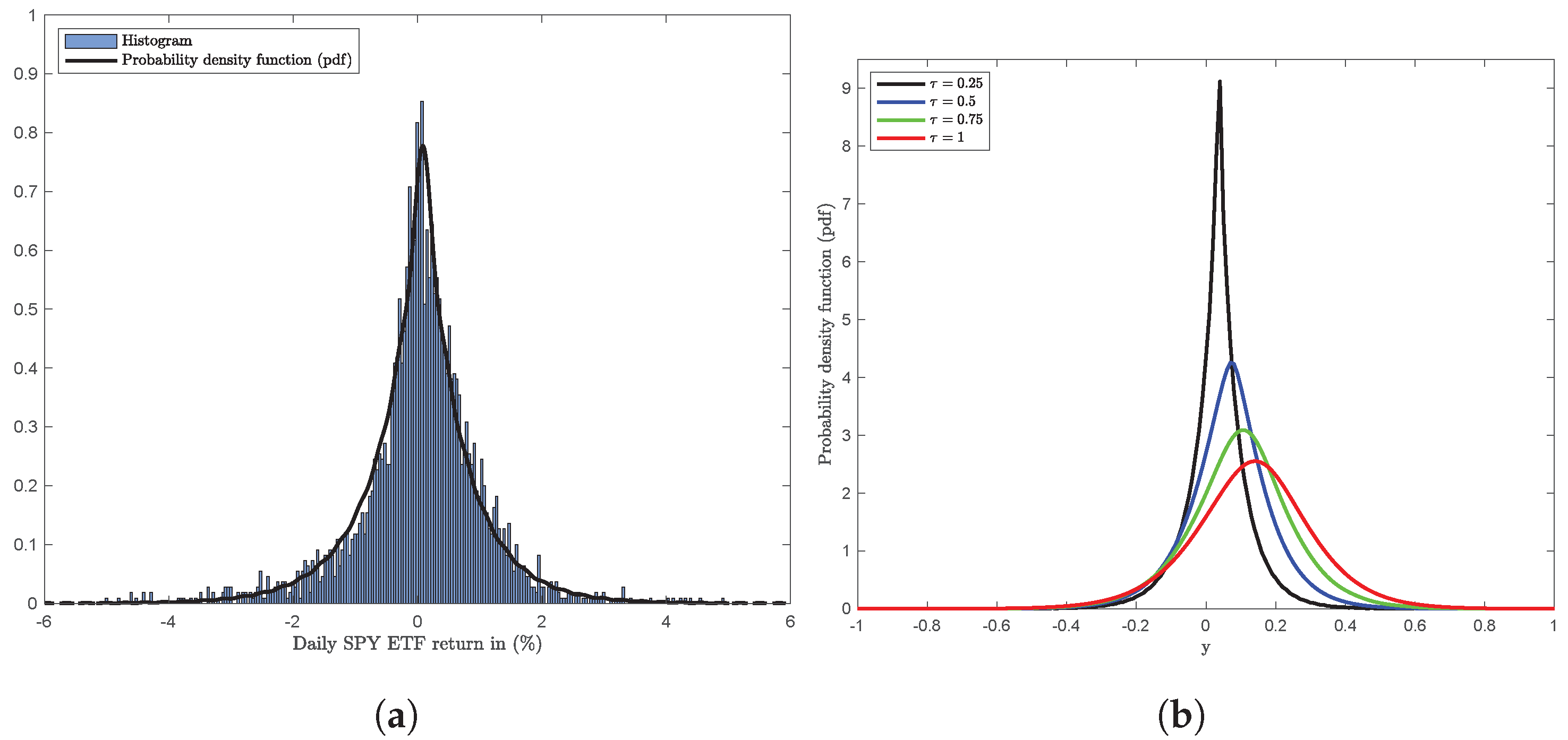
As shown in (50), the dynamic of the probability density f ( y , t ) is carried by two parameters, t μ and t α ; f ( y , t ) can be compared to the histogram of the daily SPY ETF return data, as shown in Figure 4a. Figure 4b shows the shape of the probability densities (49) adjusted at different timeframes: Quarterly ( τ = 0.25 ), Semi-Annually ( τ = 0.5 ), Third-Quarterly ( τ = 0.75 ), and Annually ( τ = 1 ).
The discrepancy between the shape of the probability densities (49) can be explained by the asymptotic distribution in Theorem 5. When the timeframe becomes large, the VG probability density generated by the Lévy Process changes its nature and becomes a normal distribution process. Empirically, the convergence is illustrated in Figure 4b.

4. Variance-Gamma Process: Pricing European Options

4.1. Variance-Gamma Process: Risk-Neutral Esscher Measure

The method of Esscher transforms introduced by Gerber and Shiu (1993) represents an efficient technique for pricing derivative securities when a Lévy process models the logarithms of the underlying asset prices. An Esscher transform of a stock price process provides an equivalent Martingale measure; under such a measure, the price of any derivative security is calculated as the expectation of the discounted payoffs. In some cases, the Esscher transform of a distribution Gerber and Shiu (1993) remains in the family of the original distributions. Gamma, Exponential, Normal, Inverse Gaussian, Negative Binomial, Geometric, Poisson, and Compound Poisson distributions are examples of conservative distributions. The existence of the equivalent Esscher transform measure is not always guaranteed, and the issue of the unicity of the equivalent Martingale measure remains recurrent when pricing an option with a Lévy process.
From the characteristic function ϕ ( ξ ) in (36), we have the moment-generating function of the VG model:
M ( h , t ) = ϕ ( i h ) t = e t μ h 1 1 2 θ σ 2 h 2 δ θ h t α = M ( h , 1 ) t with h 1 < h < h 2 M ( h , 1 ) = e μ h 1 1 2 θ σ 2 h 2 δ θ h α with h 1 < h < h 2 h 1 = δ σ 2 δ 2 σ 4 + 2 θ σ 2 h 2 = δ σ 2 + δ 2 σ 4 + 2 θ σ 2
Under the Esscher transform with parameter h, the probability density of Y = Y t becomes
f ^ ( x , t , h ) = e h x f ( x , t ) M ( h , t ) with h 1 < h < h 2
The moment-generating function of the Esscher transform VG model with h 1 < h < h 2 z is
M ( z , t , h ) = E h e z X t = 0 + e z x f ^ ( x , t , h ) d x = 0 + e ( h + z ) x f ( x , t ) M ( x , t ) d x = M ( h + z , t ) M ( h , t ) with h 1 < h < h 2 z = M ( h + z , 1 ) M ( h , 1 ) t = M ( z , 1 , h ) t
with
M ( z , 1 , h ) = M ( h + z , 1 ) M ( h , 1 ) = e μ z M * * ( z , 1 , h ) α M * * ( z , 1 , h ) = 1 1 2 θ σ 2 h 2 δ θ h 1 1 2 θ σ 2 ( h + z ) 2 δ θ ( h + z )
f ^ ( x , t , h ) is the modified probability density of f ( x , t ) defined in (49). The function e x p ( x ) is a strictly increasing function, and the probability measure generated by f ^ ( x , t , h ) is equivalent to the original probability measure generated by f ( x , t ) . Both probability measures have the same null sets Gerber and Shiu (1993) (sets with probability measure zero).
We consider the process e r τ S ( τ ) τ 0 , with r constant risk-free interest rate. We look into the necessary conditions to have h = h * such that
E h * e r τ S ( τ ) = S ( 0 ) .
From Lévy Framework and Asset Pricing in Section 2.1, we have S ( τ ) = S ( 0 ) e Y τ , with Y τ being the Variance-Gamma process. Equation (57) then becomes
e r τ = E h * e Y τ = M ( 1 , 1 , h * ) τ = M ( h * + 1 , 1 ) M ( h * , 1 ) τ with h 1 < h * < h 2 1
The first condition is that
h 2 h 1 > 1 δ 2 σ 4 + 2 θ σ 2 > 1 4
Equation (58) is equivalent to (59).
e r μ α = M * * ( 1 , 1 , h * ) = M ( h * + 1 , 1 ) M ( h * , 1 ) = 1 1 2 θ σ 2 h * 2 δ θ h * 1 1 2 θ σ 2 ( h * + 1 ) 2 δ θ ( h * + 1 )
We consider the function g ( h ) , defined as follows:
g ( h ) = 1 1 2 θ σ 2 h 2 δ θ h 1 1 2 θ σ 2 ( h + 1 ) 2 δ θ ( h + 1 )
d g d h ( h ) = 1 2 θ 2 σ 4 h 2 + δ θ 2 ( 1 2 σ 2 + δ ) h + δ θ 2 ( 1 2 σ 2 + δ ) + θ σ 2 ( 1 1 2 θ σ 2 ( h + 1 ) 2 δ θ ( h + 1 ) ) 2
and we have
d g d h ( h ) > 0 h 1 < h < h 2 1 lim h h 1 g ( h ) = 0 lim h h 2 1 g ( h ) = +
where (60) shows the existence and unicity of h * in [ h 1 , h 2 1 [ such that
e r μ α = g ( h * ) .
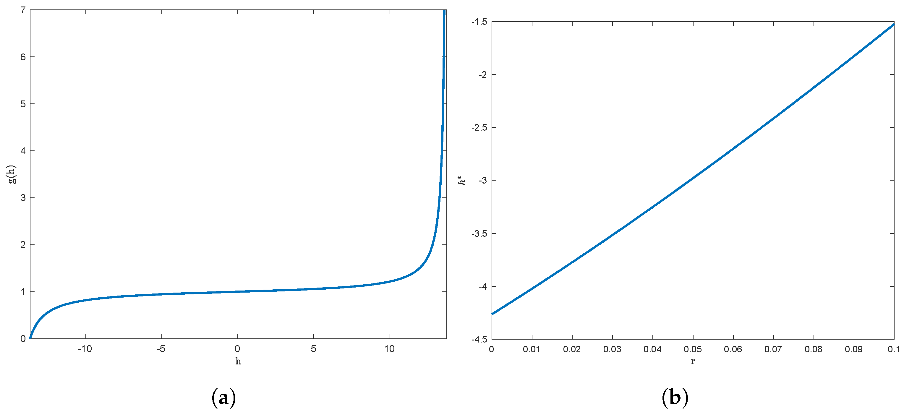
For the VG model in Table 1 Nzokem (2021a, 2021b), the existence and unicity of h * can be studied empirically, as shown in Figure 5. Over the interval [ h 1 ; h 2 1 ] , g(h) is an increasing function, as shown in Figure 5a. Figure 5b provides the solution h * of Equation (59) for a free interest rate less than 10%. The solution of h * increases with the free interest rate r.
From the Esscher transform, we have the Equivalent Martingale Measure (EMM) Q , which can be written as the Radon–Nikodym derivative:
d Q d P = e h * Y τ M ( h * , τ ) = e h * Y τ l o g ( M ( h * , τ ) )
and E Q for the expectation with respect to Q :
E Q e r τ S ( τ ) = E P e r τ S ( τ ) d Q d P = S ( 0 ) E P e ( 1 + h * ) Y τ l o g ( M ( h * , τ ) ) r τ = S ( 0 ) E P e ( 1 + h * ) Y τ e l o g ( M ( h * , τ ) ) r τ = S ( 0 ) M ( 1 + h * , τ ) M ( h * , τ ) e r τ ( 58 ) e r τ = M ( h * + 1 , τ ) M ( h * , τ ) = S ( 0 )
We have the expression (57)
E Q e r τ S ( τ ) = S ( 0 ) .
Theorem 6.
(Variance-Gamma Esscher transform distribution)
The Esscher transform of the Variance-Gamma process Y = { Y t } t 0 with parameter ( t μ , δ , σ , t α , θ ) is a Variance-Gamma process with parameter ( t μ , δ ˜ , σ , t α , θ ˜ ) :
δ ˜ = δ + h σ 2 θ ˜ = θ 1 1 2 θ σ 2 h 2 δ θ h
Proof: 
From (56), we have
M * * ( z , 1 , h ) = 1 1 2 θ σ 2 h 2 δ θ h 1 1 2 θ σ 2 ( h + z ) 2 δ θ ( h + z )
We can divide the denominator by the numerator of the function M * * ( z , 1 , h ) in (64) and rearrange the resulting expression:
M * * ( z , 1 , h ) = 1 1 1 2 θ ˜ σ 2 z 2 δ ˜ θ ˜ z θ ˜ = θ 1 1 2 θ σ 2 h 2 δ θ h δ ˜ = δ + h σ 2
M ( z , 1 , h ) in (56) becomes
M ( z , 1 , h ) = e μ z 1 1 2 θ ˜ σ 2 z 2 δ ˜ θ ˜ z α
Using the Esscher transform method, the moment-generating function for the Variance-Gamma process Y = { Y t } t 0 becomes
M ( z , t , h ) = E h e z Y t = M ( z , 1 , h ) t = e t μ z 1 1 2 θ ˜ σ 2 z 2 δ ˜ θ ˜ z t α with h ˜ 1 < z < h ˜ 2
We now have a new Variance-Gamma process with parameter ( t μ , δ ˜ , σ , t α , θ ˜ ) . □
The Esscher transform method preserves the structure of the five-parameter VG process, introduces an addition symmetric parameter ( h σ 2 ), and inflates the Gamma scale parameter by a factor of 1 1 1 2 θ σ 2 h 2 δ θ h .

4.2. Variance-Gamma Model: Extended Black–Scholes Formula

Corollary 1.
(Extended Black–Scholes)
Let r, a continuously compounded risk-free rate of interest; Y = { Y t } t 0 , a VG Process with parameter ( μ t , δ , σ , α t , θ ) ; and ( S ( 0 ) e X T K ) + , the terminal payoff for a contingent claim with expiry date T.
Then, at time t < T , the arbitrage price of a European call option with strike price K can be written as follows:
F c a l l G V ( S t , t ) = S ( t ) 1 F ^ ( l o g ( K S ( t ) ) , τ , h * + 1 ) K e r τ 1 F ^ ( l o g ( K S ( t ) ) , τ , h * )
F ^ ( l o g ( K S ( t ) ) , τ , h * ) = l o g ( K S ( t ) ) f ^ ( ξ , τ , h * ) d ξ f ^ ( ξ , τ , h * ) in ( 54 )
where τ = T t and F ^ ( k , τ , h * ) and F ^ ( k , τ , h * + 1 ) are the cumulative distribution of the VG models with parameters ( τ μ , δ ˜ , σ , τ α , θ ˜ ) and ( τ μ , δ ˜ + σ 2 , σ , τ α , θ ˜ e r μ α ) , respectively.
Proof: 
f ( Y T , K ) = ( S ( 0 ) e Y T K ) + = S ( t ) ( e Y τ k ) + Y T = Y τ + Y t = S ( t ) g ( Y τ ) S ( t ) = S ( 0 ) e Y t and k = K S ( t )
Under the Equivalent Martingale Measure (EMM), f ^ ( ξ , τ , h * ) is the probability density of the VG model with parameter ( τ μ , δ ˜ , σ , τ α , θ ˜ ) . We note that k = K S ( t ) .
S ( t ) e r τ l o g ( k ) + e ξ f ^ ( ξ , τ , h * ) d ξ = S ( t ) e r τ l o g ( k ) + e ξ e h * ξ f ( ξ , τ ) M ( h , t ) d ξ f ^ ( ξ , τ , h * ) in ( 54 ) = S ( t ) e r τ l o g ( k ) + e ( 1 + h * ) ξ f ( ξ , τ ) M ( h * , t ) d ξ e r τ = M ( h * + 1 , τ ) M ( h * , τ ) in ( 58 ) = S ( t ) l o g ( k ) + e ( 1 + h * ) ξ f ( ξ , τ ) M ( 1 + h * , t ) d ξ = S ( t ) l o g ( k ) + f ^ ( ξ , τ , h * + 1 ) d ξ
We can now show the relation in (68):
F c a l l G V ( S t , t ) = S ( t ) e r τ E Q g ( X τ ) = S ( t ) e r τ + f ^ ( ξ , τ , h * ) ( e ξ k ) + d y = S ( t ) e r τ l o g ( k ) + e ξ f ^ ( ξ , τ , h * ) d ξ K e r τ l o g ( k ) + f ^ ( ξ , τ , h * ) d ξ = S ( t ) l o g ( k ) + f ^ ( ξ , τ , h * + 1 ) d ξ K e r τ l o g ( k ) + f ^ ( ξ , τ , h * ) d ξ = S ( t ) 1 F ^ ( l o g ( k ) , τ , h * + 1 ) K e r τ 1 F ^ ( l o g ( k ) , τ , h * )
with
F ^ ( l o g ( k ) , τ , h * ) = l o g ( k ) f ^ ( ξ , τ , h * ) d ξ F ^ ( l o g ( k ) , τ , h * + 1 ) = l o g ( k ) f ^ ( ξ , τ , h * + 1 ) d ξ
From Theorems 4 and 6, f ^ ( ξ , τ , h * ) is the probability density of the VG model with parameter ( τ μ , δ ˜ , σ , τ α , θ ˜ ) .
f ^ ( ξ , τ , h * ) = 1 σ Γ ( τ α ) θ ˜ τ α 0 + 1 2 π v e ( y μ δ ˜ v ) 2 2 v σ 2 v τ α 1 e v θ ˜ d v ( δ ˜ , θ ˜ ) in ( 63 )
Following the same methodology, f ^ ( ξ , τ , h * + 1 ) is the probability density of the VG model with parameter ( τ μ , δ ˜ , σ , τ α , θ ˜ ) . Thus, we have
δ ˜ = δ ˜ + σ 2 θ ˜ = θ ˜ e r μ α
In fact, as in (70), we have
δ ˜ = δ + ( h * + 1 ) σ 2 = δ ˜ + σ 2
and
θ ˜ = θ 1 1 2 θ σ 2 ( h * + 1 ) 2 δ θ ( h * + 1 ) = θ 1 1 2 θ σ 2 h * 2 δ θ h * e r μ α = θ ˜ e r μ α
We have the probability density,
f ^ ( ξ , τ , h * + 1 ) = 1 σ Γ ( τ α ) θ ˜ τ α 0 + 1 2 π v e ( y μ δ ˜ v ) 2 2 v σ 2 v τ α 1 e v θ ˜ d v

Equivalent Martingale Measure (EMM) Computation

Under the Equivalent Martingale Measure (EMM), f ^ ( ξ , τ , h * ) is the probability density of the VG model with parameter ( τ μ , δ ˜ , σ , τ α , θ ˜ ) . The Fourier transform is
F [ f ^ ] ( y , τ , h * ) = E e i y X τ = e i μ y 1 + 1 2 θ ˜ σ 2 y 2 + i δ ˜ θ ˜ y α τ see ( 67 ) = ϕ ( y ) τ = e τ l o g ( ϕ ( y ) ) = e τ φ ( y )
F [ f ^ ] ( y , τ , h * ) = e τ φ ( y ) φ ( y ) = i μ y + α l o g ( 1 + 1 2 θ ˜ σ 2 y 2 i δ ˜ θ ˜ y )
where ϕ ( y ) is defined in (36) and φ ( y ) is the characteristic exponent of the VG model with parameter ( μ , δ ˜ , σ , α , θ ˜ ) .
f ^ ( ξ , τ , h * ) can be written as the inverse Fourier Transform from (73):
f ^ ( ξ , τ , h * ) = 1 2 π + e i ξ z F [ f ^ ] ( z , τ , h * ) d z = 1 2 π + e i ξ z τ φ ( z ) d z = 1 2 π + e i ξ z τ φ ( z ) d z
It was shown in Nzokem (2021a) that we can have
F [ F ^ ] ( ξ , τ , h * ) = F [ f ^ ] ( ξ , τ , h * ) i ξ + π F [ f ^ ] ( 0 ) δ ( ξ ) .
Based on (74), we can deduce that
F ^ ( ξ , τ , h * ) = 1 2 π + e i ξ z F [ F ^ ] ( z , τ , h * ) d z = 1 2 π + e i ξ z τ φ ( z ) i z d z + 1 2
We have the probability density and cumulative functions:
f ^ ( ξ , τ , h * ) = 1 2 π + e i ξ z τ φ ( z ) d z F ^ ( ξ , τ , h * ) = 1 2 π + e i ξ z τ φ ( z ) i z d z + 1 2
The Fractional Fast Fourier Transform (FRFT) Nzokem (2021a) was used to compute f ^ ( ξ , τ , h * ) and f ^ ( ξ , τ , h * + 1 ) in (75). The results are shown in Figure 6b and Figure 7b.
The twelve-point rule Composite Newton–Cotes Quadrature Formulas Nzokem (2020, 2021c) was also used to compute f ^ ( ξ , τ , h * ) and f ^ ( ξ , τ , h * + 1 ) . This method relies on the numerical integration technique and aims to estimate the density function as follows:
f ^ ( ξ , τ , h ) b n p = 0 n Q 1 j = 0 Q W j g ( x Q p + j , τ , h ) g ( x , τ , h ) = 1 σ θ ˜ τ α Γ ( τ α ) 2 π e ( x τ μ δ ˜ v ) 2 2 v σ 2 v τ α 1 2 e v θ ˜
For the VG model in Table 1 Nzokem (2021a, 2021b) with μ ^ = 0.0848 , δ ^ = 0.0577 , σ ^ = 1.0295 , α ^ = 0.8845 , and θ ^ = 0.9378 ; we added a 6 % risk-free interest rate and computed the Esscher transform parameter ( h * = 2.6997 ) from (58). In order to perform the computation in (76), the following parameter values were used a = 0 , b = 20 , Q = 12 , n = 5000 Q , n 0 = 5000 ; and the weight values { W j } 0 j Q come from Table 1 Nzokem (2021c) and Table 4.1 Nzokem (2020). The estimation results are shown in Figure 6a and Figure 7a.
Both methods produce smooth density functions, as shown in Figure 6 and Figure 7. Figure 6c and Figure 7c provide the estimation error of f ^ ( ξ , τ , h * + 1 ) . Fractional Fast Fourier (FRFT) underestimates the peakedness of the density function when the timeframe is small ( τ = 0.25 years), as shown in Figure 6c. The estimation error decreases significantly when the timeframe increases; see Figure 7c when τ = 0.5 years.
Both methods will be implemented in the empirical analysis section to produce the arbitrage price of a European call option.

4.3. Variance-Gamma Model: Generalized Black–Scholes Formula

Theorem 7.
(Generalized Black–Scholes)
Let r, a continuously compounded risk-free rate of interest; Y = { Y t } t 0 , a VG Process with parameter ( μ t , δ , σ , α t , θ ) ; and ( S ( 0 ) e X T K ) + , the terminal payoff for a contingent claim with expiry date T. Then, at time t < T , the arbitrage price of a European call option with strike price K can be written as follows:
F c a l l G V ( S t , t ) = K 2 π + i q + + i q e i ξ l o g ( S ( t ) K ) τ ( r + φ ( ξ ) ) i ξ ( i ξ 1 ) d ξ
where φ ( z ) is the characteristic exponent of the VG model with parameter ( μ , δ ˜ , σ , α , θ ˜ ) in (63), τ = T t , and q < 1 .
Proof: 
( S ( 0 ) e Y T K ) + = S ( t ) ( e Y τ k ) + Y T = Y τ + Y t
= S ( t ) g ( Y τ , k ) S ( t ) = S ( 0 ) e Y t and k = K S ( t )
where ( S ( 0 ) e Y T K ) + is the payoff of the call option. The Fourier transform can be written as
F [ g ] ( y , k ) = 0 + e i y x g ( x , k ) d x = 0 + e i y x ( e x k ) + d x = l o g ( k ) + e i y x ( e x k ) d x = l o g ( k ) + e ( 1 i y ) x d x k l o g ( k ) + e i y x d x = 1 1 i y e ( 1 i y ) x l n ( k ) + + k i y e i y x l n ( k ) + = k e i y l o g ( k ) i y ( i y 1 ) for ( y ) < 1
We have the Fourier transform of the call payoff
g ^ ( y , k ) = F [ g ] ( y , k ) = k e i y l o g ( k ) i y ( i y 1 ) for ( y ) < 1
It is shown in (75) and (73) that f ^ ( ξ , τ , h * ) and φ ( y ) can be written as follows:
f ^ ( ξ , τ , h * ) = 1 2 π + e i ξ z τ φ ( z ) d z φ ( y ) = i μ y + α l o g ( 1 + 1 2 θ ˜ σ 2 y 2 i δ ˜ θ ˜ y )
with ( δ ˜ , θ ˜ ) defined as in (63).
F c a l l G V ( S t , t ) is the call option price under the Equivalent Martingale Measure (EMM), and we have the following expression.
F c a l l G V ( S t , t ) = e r τ E h * ( S ( 0 ) e X T K ) + = S ( t ) e r τ E h * g ( X τ ) ( recall ( 79 ) = S ( t ) e r τ + f ^ ( y , τ , h * ) g ( y , k ) d y = S ( t ) 2 π + + e i y z τ ( r + φ ( z ) ) g ( y , k ) d y d z = S ( t ) 2 π + e τ ( r + φ ( z ) ) g ^ ( z , k ) d z recall ( 80 ) = K 2 π + i q + + i q e x p i z l o g ( k ) τ ( r + φ ( z ) ) ) i z ( i z 1 ) d z ( z ) q < 1 and k = K S ( t ) = K 2 π + i q + + i q e x p i z l o g ( S ( t ) K ) τ ( r + φ ( z ) ) i z ( i z 1 ) d z
We have the following formula (77):
F c a l l G V ( S t , t ) = K 2 π + i q + + i q e x p i z l o g ( S ( t ) K ) τ ( r + φ ( z ) ) i z ( i z 1 ) d z

4.4. European Option Pricing by Fractional Fast Fourier Transform (FRFT)

4.4.1. Evaluation of Parameter q

We consider a stock or index price S = S 0 e Y and a strike price K; it was shown in (80) that the Fourier transform of the call payoff can be written as follows:
g ^ ( y , k ) = F [ g ] ( y , k ) = k e i y l o g ( k ) i y ( i y 1 ) for ( y ) < 1
We can recover the call payoff from the inverse Fourier in (80):
g ˇ ( x , k ) = 1 2 π + i q + + i q e i y x F [ g ] ( y , k ) d y for q < 1
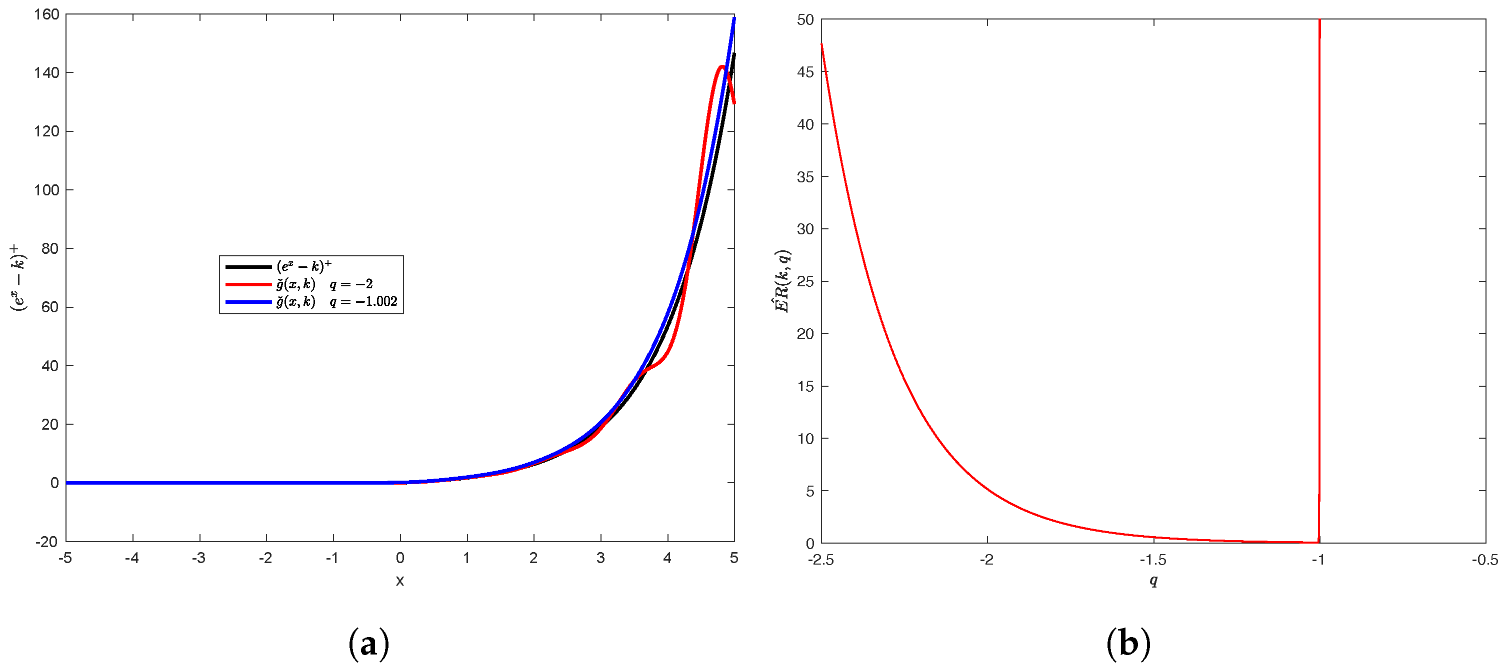
The payoff in (83) depends on the q parameter. As shown in Figure 8a, for q = 2 , the inverse Fourier in (83) produces poor results; in fact, the curve in red fluctuates around the real call payoff ( e Y k ) + . For q = 1.002 , the inverse Fourier overestimates the call payoff.
To find a value of q that results in high accuracy, we define the error function ( E R ( k , q ) ) between the real call payoff and the inverse Fourier payoff, with k (strike price) and the q parameter as inputs:
E R ( k , q ) = 1 m j = 1 m ( e x j k ) + g ˇ ( x j , k ) 2 with M x j M
For an at-the-money (ATM) option, the strike price k = 1 and E R ( k , q ) can be analyzed as a function of one variable q. Figure 8b displays the error ( E R ) as a function of q. E R is a convex function that decreases and increases over the interval ] , 1 [ . The section method was applied to determine q * = 1.0086 , which minimizes E R ( 1 , q * ) .
Figure 9a displays the E R ( k , q * ) minimum value as a function of strike price k; and Figure 9b displays the correspondent optimal parameter q * as a function of strike price k. Both graphs display almost a constant function with respect to strike price.

4.4.2. Calculating the Fourier Integral by FRFT

The Fourier transform method Li et al. (2020) provides valuable and powerful tools for option pricing under a class of Lévy processes when the characteristic function is much simpler than the density function. We can compute the call option’s value on the SPY ETF with the Fractional Fast Fourier Transform (FRFT).
For x = l o g ( S ( t ) K ) , F c a l l G V ( S ( t ) , t ) K is the price per one dollar of the strike price. We have
F c a l l G V ( S t , τ ) K = 1 2 π + i q + + i q e x p i z l o g ( S ( t ) K ) τ ( r + φ ( z ) ) i z ( i z 1 ) d z = 1 2 π + i q + + i q e i z x e x p τ ( r + φ ( z ) ) i z ( i z 1 ) d z
and we assume that
f ( ξ ) = e x p τ ( r + φ ( z ) ) i ξ ( i ξ 1 ) F ( x ) = 1 2 π + i q + + i q e i ξ x f ( ξ ) d ξ
Based on the Fractional Fast Fourier (FRFT) notations in Nzokem (2021a) (Section 2 and Appendix A.1), we have developed the following approximation
F ( x k ) = 1 2 π + i q + + i q e i ξ x k f ( ξ ) d ξ = e q x k 2 π + e i ξ x k f ( ξ + i q ) d ξ e q x k 2 π a 2 a 2 e i ξ x k f ( ξ + i q ) d ξ γ 2 π e ( q + m 2 β ) x k G k ( f ( ξ j + i q ) e π i j n δ , δ )
F ( x k ) γ 2 π e ( q + m 2 β ) x k G k ( f ( ξ j + i q ) e π i j n δ , δ )

4.5. Empirical Analysis

Based on parameter data from the VG model Nzokem (2021a, 2021b) with μ ^ = 0.0848 , δ ^ = 0.0577 , σ ^ = 1.0295 , α ^ = 0.8845 , and θ ^ = 0.9378 , we added a 6 % risk-free interest rate and computed the Esscher transform parameter ( h * = 2.6997 ). The VG option pricing is calculated across maturity and option moneyness using the extended and generalized Black–Scholes formulas. The closed-form Black–Scholes model Hull (2003) was added to the analysis as a benchmark.
F c a l l B S ( S t , τ ) = S t N ( d 1 ) K e r τ N ( d 2 ) d 1 = L n ( S t K ) + ( r + 1 2 σ * 2 ) τ σ * τ d 2 = d 1 σ * τ N ( x ) = 1 2 π x exp t 2 2 d t
The variance σ * 2 = 0.1848 is the annualized variance computed from the daily SPY ETF return variance in Nzokem (2021a).
Option Moneyness describes the intrinsic value of an option in its current state. It indicates whether the option would make money if exercised immediately. Option moneyness can be classified into three categories: At-The-Money (ATM) options ( k = S t K = 1 ), Out-of-The Money (OTM) options ( k = S t K < 1 ), and In-The-Money (ITM) options ( k = S t K > 1 ). On 4 August 2021, the SPY ETF market price closed at 438.98 . We compute the VG call option price on SPY ETF using the spot price ( S 0 ) 438.98 . The results are summarised in Table 3.
The Fractional Fourier Transform (FRFT) algorithm performs poorly for in-the-money (ITM) options. The FRFT underprices the VG for in-the-money (ITM) options, whereas the twelve-point rule Composite Newton–Cotes Quadrature produces consistent option pricing results with the Black–Scholes model. Both algorithms yield consistent results for at-the-money and out-of-the-money options.
To generalize the analysis and account for a large range of option moneyness and maturity, The error (88) was computed as the difference between VG and BS option prices:
E r r o r ( k , τ ) = F c a l l G V ( S t , τ ) K F c a l l B S ( S t , τ ) K ( k = S t K )
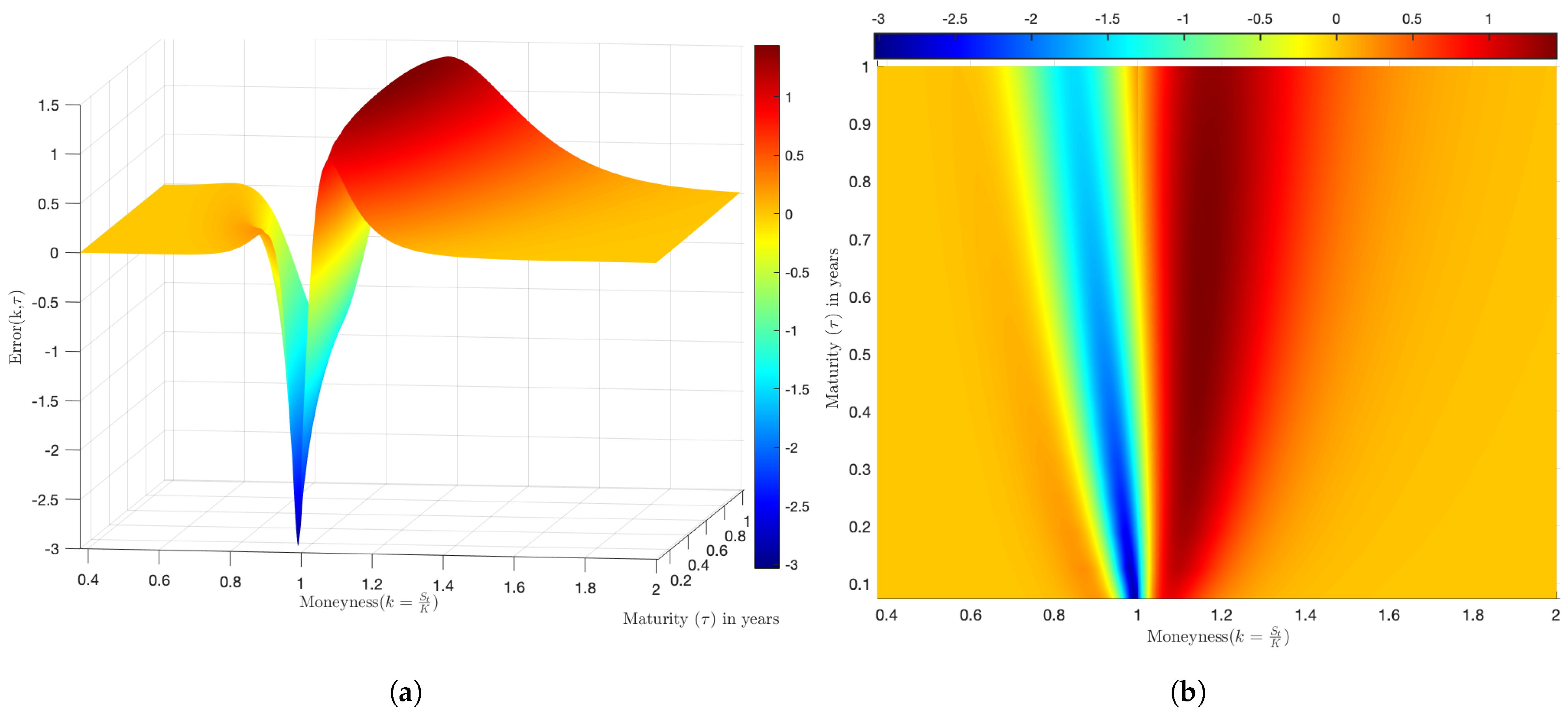
Figure 10 displays the error E r r o r ( k , τ ) as a function of the time to maturity ( τ ) and the option moneyness (k). The spot price ( S t ) is a constant, and the option moneyness depends on the strike price.
The Black–Scholes (BS) and VG models produce different option pricing results. The Black–Scholes model is overpriced for out-of-the-money (OTM) options (indicated by blue in Figure 10) and underpriced for the in-the-money (ITM) options (indicated by red in Figure 10).
The results shown in Figure 10 are consistent with Mozumder et al. (2015), where VG pricing was performed on S&P500 index data. The shape in Figure 10a looks similar to that in Figure 6 in Mozumder et al. (2015), with the option Moneyness variable replacing the strike price. However, the overpriced Black–Scholes model, shown in blue in (Figure 10), does not support the findings in Madan and Milne (1991) that VG option prices are typically higher than Black–Scholes model prices, with the percentage bias rising when the stock is out-of-the-money (OTM). One of the limitations of these studies is that the VG model is symmetric and uses three parameters; the five-parameter VG model controls the excess kurtosis and the skewness of the daily SPY ETF return data.

5. Conclusions

In the paper, a Γ ( α , θ ) Ornstein–Uhlenbeck type process was used to build a continuous sample path of a five-parameter Variance-Gamma (VG) process ( μ , δ , σ , α , θ ): location ( μ ), symmetry ( δ ), volatility ( σ ), shape ( α ), and scale ( θ ). The data parameters Nzokem (2021a, 2021b) were used to simulate the gamma process ( σ 2 ( t ) ) and the continuous sample path of the subordinator process ( σ 2 * ( t ) ). Both simulations were used as inputs to simulate the continuous sample path of the VG process. The Lévy density of the VG process was derived and shown to belong to a KoBoL family of order ν = 0 , intensity α , and steepness parameters δ σ 2 δ 2 σ 4 + 2 θ σ 2 and δ σ 2 + δ 2 σ 4 + 2 θ σ 2 . We have shown that the VG process converges asymptotically in distribution to a Lévy process driven by a normal distribution with mean ( μ + α θ δ ) and variance α ( θ 2 δ 2 + σ 2 θ ) . The existence of the Equivalent Martingale Measure (EMM) of the five-parameter VG process was also shown. The EMM preserves the structure of the five-parameter VG process, with an inflated Gamma scale parameter and a constant term adjustment symmetric parameter. The extended Black–Scholes formula provides the closed form of the VG option price. The Lévy process generated by the VG model provides the generalized Black–Scholes formula. The daily SPY ETF return data illustrate the computation of European option pricing under the five-parameter VG process. The twelve-point rule Composite Newton–Cotes Quadrature and Fractional Fast Fourier Transform (FRFT) algorithms were implemented to compute the European option price. The results show that the FRFT yields inconsistent European option prices for in-the-money options. The Black–Scholes (BS) and VG models produce different option pricing results. The Black–Scholes model is overpriced for out-of-the-money (OTM) options and underpriced for in-the-money (ITM) options. However, for deep out-of-the-money (OTM) and deep in-the-money (ITM) options, the Black–Scholes and VG models yield almost the same option prices.

Funding

The paper receives no external funding.

Institutional Review Board Statement

Not applicable.

Informed Consent Statement

Not applicable.

Data Availability Statement

The author confirms that the data supporting the findings of this study are available within the article Nzokem (2021a, 2021b).

Conflicts of Interest

The author declares no conflict of interest.

References

  1. Adeosun, Mabel E., Sunday O. Edeki, and Olabisi O. Ugbebor. 2016. On a variance gamma model (vgm) in option pricing: A difference of two gamma processes. Journal of Informatics and Mathematical Sciences 8: 1–16. [Google Scholar]
  2. Alhagyan, Mohammed, Masnita Misiran, and Zurni Omar. 2020. Discussions on continuous stochastic volatility models. Global and Stochastic Analysis 7: 55–64. [Google Scholar]
  3. Andrusiv, Andrii, and Hans-Jürgen Engelbert. 2020. On the minimal entropy martingale measure for lévy processes. Stochastics 92: 1223–43. [Google Scholar] [CrossRef]
  4. Applebaum, David. 2009. Lévy Processes and Stochastic Calculus. Cambridge: Cambridge University Press. [Google Scholar]
  5. Arias-de Reyna, Juan. 1990. On the theorem of frullani. Proceedings of the American Mathematical Society 109: 165–75. [Google Scholar] [CrossRef]
  6. Barndorff-Nielsen, Ole E., and Neil Shephard. 2001a. Modelling by lévy processes for financial econometrics. In Lévy Processes. Boston: Birkhäuser, pp. 283–318. [Google Scholar]
  7. Barndorff-Nielsen, Ole E., and Neil Shephard. 2001b. Non-gaussian Ornstein–uhlenbeck-based models and some of their uses in financial economics. Journal of the Royal Statistical Society: Series B (Statistical Methodology) 63: 167–241. [Google Scholar] [CrossRef]
  8. Barndorff-Nielsen, Ole E., and Neil Shephard. 2002. Financial Volatility, Lévy Processes and Power Variation. Oxford: Nuffield College, Unpublished book. [Google Scholar]
  9. Barndorff-Nielsen, Ole E., and Neil Shephard. 2003. Integrated ou processes and non-gaussian ou-based stochastic volatility models. Scandinavian Journal of Statistics 30: 277–95. [Google Scholar] [CrossRef] [Green Version]
  10. Barndorff-Nielsen, Ole E., Jens Ledet Jensen, and Michael Sørensen. 1998. Some stationary processes in discrete and continuous time. Advances in Applied Probability 30: 989–1007. [Google Scholar] [CrossRef]
  11. Black, Fischer, and Myron Scholes. 1973. The pricing of options and corporate liabilities. Journal of Political Economy 81: 637–54. [Google Scholar] [CrossRef] [Green Version]
  12. Boyarchenko, Svetlana, and Sergei Z. Levendorskii. 2002. Non-Gaussian Merton-Black-Scholes Theory. Singapore: World Scientific, vol. 9. [Google Scholar]
  13. Carr, Peter, Hélyette Geman, Dilip B. Madan, and Marc Yor. 2003. Stochastic volatility for lévy processes. Mathematical Finance 13: 345–82. [Google Scholar] [CrossRef] [Green Version]
  14. Cont, Rama. 2001. Empirical properties of asset returns: Stylized facts and statistical issues. Quantitative Finance 1: 223–36. [Google Scholar] [CrossRef]
  15. Gerber, Hans U., and Elias S. W. Shiu. 1993. Option pricing by Esscher Transforms. Paris: HEC Ecole des Hautes Études Commerciales. [Google Scholar]
  16. Heston, Steven L. 1993. A closed-form solution for options with stochastic volatility with applications to bond and currency options. The Review of Financial Studies 6: 327–43. [Google Scholar] [CrossRef] [Green Version]
  17. Hull, John, and Alan White. 1987. The pricing of options on assets with stochastic volatilities. The Journal of Finance 42: 281–300. [Google Scholar] [CrossRef]
  18. Hull, John C. 2003. Options Futures and Other Derivatives. Toronto: Pearson Education India. [Google Scholar]
  19. Kendall, Maurice George. 1946. The Advanced Theory of Statistics, 2nd ed. London: Charles Griffin. [Google Scholar]
  20. Ken-Iti, Sato. 1999. Lévy Processes and Infinitely Divisible Distributions. Cambridge: Cambridge University Press. [Google Scholar]
  21. Kou, Steven G. 2002. A jump-diffusion model for option pricing. Management Science 48: 1086–101. [Google Scholar] [CrossRef] [Green Version]
  22. Kyprianou, Andreas E. 2014. Fluctuations of Lévy Processes with Applications: Introductory Lectures. Berlin: Springer Science & Business Media. [Google Scholar]
  23. Li, Cuixiang, Huili Liu, Mengna Wang, and Wenhan Li. 2020. The pricing of compound option under variance gamma process by FFT. Communications in Statistics-Theory and Methods 50: 6122–36. [Google Scholar] [CrossRef]
  24. Madan, Dilip B., and Frank Milne. 1991. Option pricing with VG martingale components 1. Mathematical Finance 1: 39–55. [Google Scholar] [CrossRef] [Green Version]
  25. Madan, Dilip B., Peter P. Carr, and Eric C. Chang. 1998. The variance gamma process and option pricing. Review of Finance 2: 79–105. [Google Scholar] [CrossRef] [Green Version]
  26. Matsuda, Kazuhisa. 2004. Introduction to Merton Jump Diffusion Model. New York: Department of Economics, The Graduate Center, The City University of New York. [Google Scholar]
  27. Mozumder, Sharif, Ghulam Sorwar, and Kevin Dowd. 2015. Revisiting variance gamma pricing: An application to s&p500 index options. International Journal of Financial Engineering 2: 1550022. [Google Scholar]
  28. Nzokem, Aubain H. 2020. Stochastic and Renewal Methods Applied to Epidemic Models. Ph.D. Thesis, York University, YorkSpace Institutional Repository, Toronto, ON, Canada. [Google Scholar]
  29. Nzokem, Aubain H. 2021a. Fitting infinitely divisible distribution: Case of gamma-variance model. arXiv arXiv:2104.07580. [Google Scholar]
  30. Nzokem, Aubain H. 2021b. Gamma variance model: Fractional Fourier Transform (FRFT). Journal of Physics: Conference Series 2090: 012094. [Google Scholar] [CrossRef]
  31. Nzokem, Aubain H. 2021c. Numerical solution of a gamma—Integral equation using a higher order composite newton-cotes formulas. Journal of Physics: Conference Series 2084: 012019. [Google Scholar] [CrossRef]
  32. Nzokem, Aubain H. 2021d. Sis epidemic model: Birth-and-death Markov chain approach. International Journal of Statistics and Probability 10: 10–20. [Google Scholar] [CrossRef]
  33. Nzokem, Aubain H., and Montshiwa Volition T. 2022. Fitting generalized tempered stable distribution: Fractional Fourier Transform (FRFT) approach. arXiv arXiv:2205.00586. doi:10.1007/978-981-19-8406-8_34. [Google Scholar] [CrossRef]
  34. Protter, Philip. 2005. Stochastic Integration and Differential Equations. A New Approach. Berlin: Springer, vol. 21. [Google Scholar] [CrossRef]
  35. Tankov, Peter. 2003. Financial Modelling with Jump Processes. New York: Chapman and Hall/CRC. [Google Scholar] [CrossRef]
  36. Uhlenback, George E., and Leonard S. Ornstein. 1930. On the theory of the Brownian motion. Physical Review 36: 823–41. [Google Scholar] [CrossRef]
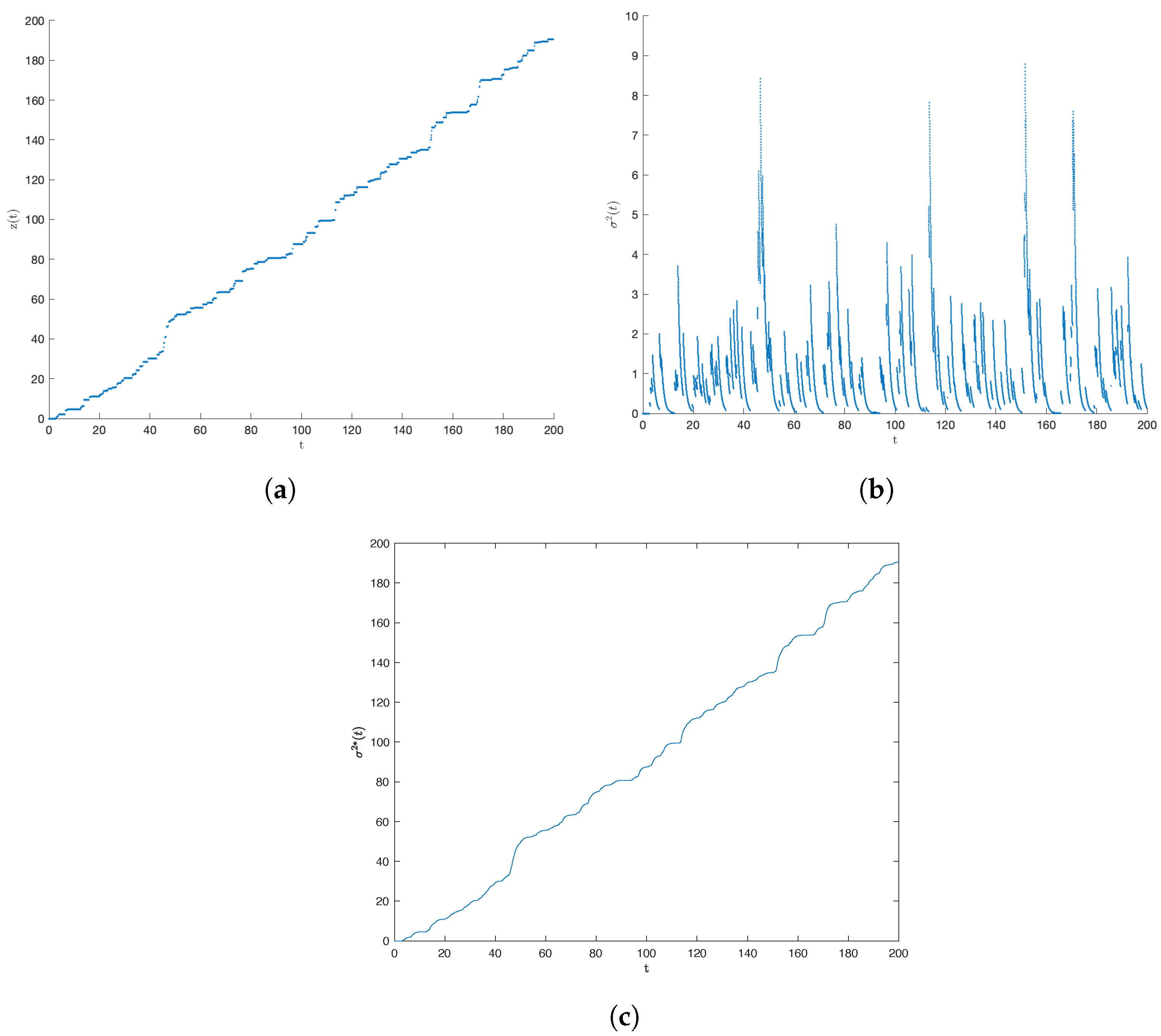
Figure 1. Simulations with α ^ = 0.8845 , θ ^ = 0.9378 : (a) compound Poisson process, z ^ ( t ) ; (b) Gamma process, σ ^ 2 ( t ) ; (c) subordinator, σ ^ 2 * ( t ) .
Jrfm 16 00055 g001
Figure 2. Simulations (with Y * = { Y t * } ) versus SPY ETF data: μ ^ = 0.0848 , δ ^ = 0.0577 , σ ^ = 1.0295 , α ^ = 0.8845 , θ ^ = 0.9378 .
Jrfm 16 00055 g002
Figure 3. VG model: μ ^ = 0.0848 , δ ^ = 0.0577 , σ ^ = 1.0295 , α ^ = 0.8845 , θ ^ = 0.9378 : (a) Lévy density of the VG model and (b) Probability density of the VG model.
Jrfm 16 00055 g003
Figure 4. f ( y , t ) with μ ^ = 0.0848 , δ ^ = 0.0577 , σ ^ = 1.0295 , α ^ = 0.8845 , θ ^ = 0.9378 : (a) daily SPY ETF return in (%) and (b) f ( y , τ ) : τ in years.
Jrfm 16 00055 g004
Figure 5. VG model with μ ^ = 0.0848 , δ ^ = 0.0577 , σ ^ = 1.0295 , α ^ = 0.8845 , θ ^ = 0.9378 , h 1 = 13.6511 , and h 2 = 14.7399 : (a) g ( h ) ; (b) e r μ α = g ( h ) .
Jrfm 16 00055 g005
Figure 6. Estimation of f ^ ( ξ , τ , h * ) versus f ^ ( ξ , τ , h * + 1 ) , τ = 0.25 : (a) Newton–Cotes Martingale; (b) FRFT Martingale Measure; (c) error: FRFT versus Newton.
Jrfm 16 00055 g006
Figure 7. Estimation of f ^ ( ξ , τ , h * ) versus f ^ ( ξ , τ , h * + 1 ) , τ = 0.5 : (a) Newton–Cotes Martingale; (b) FRFT Martingale Measure; (c) error: FRFT versus Newton.
Jrfm 16 00055 g007
Figure 8. Optimal value of q parameter: (a) ( e x k ) + versus g ˇ ( x , k ) ; (b) E R ( k , q ) and q.
Jrfm 16 00055 g008
Figure 9. Optimal q parameter and Error E R ( k , q ) values: (a) E R ( k , q * ) minimum value; (b) optimal q * parameter.
Jrfm 16 00055 g009
Figure 10. Combined effects of Time to Maturity ( τ ) and option Moneyness ( k = S t K ): (a) error (k, τ ) and (b) error (k, τ ) (top view).
Jrfm 16 00055 g010
Table 1. FRFT Maximum Likelihood VG parameter estimation.
ModelParametersStatistics
μ ^ = 0.0848 E ( Y ) ^ = 0.0369
δ ^ = 0.0577 V a r ( Y ) ^ = 0.8817
VG σ ^ = 1.0295 S k e w ( Y ) ^ = 0.173
α ^ = 0.8845 K u r t ( Y ) ^ = 6.412
θ ^ = 0.9378
Source: Nzokem (2021a, 2021b).
Table 2. Results of VG model parameter estimation.
Iterations μ δ σ α θ Log ( ML ) | | dLog ( ML ) dV | |
100111−3582.8388598.743231
20.05905599−0.00094451.031959030.91302081.03208412−3561.5099833.530396
30.069499250.004000351.041014440.884788951.05131996−3559.5656447.807305
40.075140390.000557711.175773970.673264291.17778666−3569.6221211.365781
50.08928373−0.02637161.037563210.838426610.94304967−3554.4434498.289445
60.08676498−0.05218871.033370150.855918750.95066351−3550.6419204.467192
70.086995−0.06085171.027889370.873826210.95054954−3549.846566.8039738
80.08542912−0.0585471.027052410.882584110.94321299−3549.702315.3209117
90.08478622−0.05766541.029951660.884477910.93670036−3549.69211.14764198
100.08477798−0.05777361.029223080.884490720.93831041−3549.6920.17287708
110.08476475−0.05772711.029603430.884504340.93755549−3549.6920.07850459
120.08477094−0.05774881.029426080.88449840.93790784−3549.6920.03723941
130.08476804−0.05773861.029509370.884501170.93774266−3549.6920.01732146
140.0847694−0.05774341.029470430.884499870.93781995−3549.6920.00813465
150.08476876−0.05774111.029488680.884500480.93778375−3549.6920.00380345
160.08476906−0.05774221.029480140.884500190.9378007−3549.6920.00178206
170.08476892−0.05774171.029484140.884500330.93779276−3549.6920.00083415
180.08476898−0.05774191.029482260.884500260.93779648−3549.6920.00039063
190.08476895−0.05774181.029483140.884500290.93779474−3549.6920.00018289
200.08476897−0.05774191.029482730.884500280.93779555−3549.692 8.56 10 5
210.08476896−0.05774181.029482920.884500290.93779517−3549.692 4.01 10 5
Table 3. Price of European call option on SPY ETF.
Strike PriceMoneynessBSMVGM (68)VGM (77)BSMVGM (68)VGM (77)BSMVGM (68)VGM (77)BSMVGM (68)VGM (77)BSMVGM (68)VGM (77)BSMVGM (68)VGM (77)
Period (In Year)0.06250.1250.250.50.751
219.492.00220.31220.28219.86221.13221.10220.48222.76222.72221.71225.98225.93224.14229.15229.13226.53232.27232.26228.88
225.121.95214.70214.74214.10215.54215.58214.74217.21217.25216.01220.52220.54218.53223.77223.82221.01226.97227.04223.45
231.041.90208.80208.83208.18209.66209.69208.84211.38211.41210.16214.77214.80212.77218.10218.16215.34221.39221.47217.88
237.291.85202.58202.53202.10203.47203.42202.79205.23205.18204.16208.71208.67206.86212.13212.13209.53215.51215.53212.16
243.881.80196.02196.06195.38196.92196.97196.10198.73198.78197.51202.31202.37200.32205.83205.93203.10209.31209.43205.84
250.851.75189.07189.16188.47190.01190.10189.21191.87191.96190.68195.55195.66193.61199.17199.33196.50202.75202.94199.36
258.221.70181.72181.81181.36182.69182.78182.13184.60184.69183.66188.39188.52186.70192.12192.30189.71195.81196.03192.70
266.051.65173.93173.98173.53174.92174.97174.33176.89176.95175.92180.79180.91179.09184.64184.83182.24188.45188.69185.37
274.361.60165.64165.64165.45166.67166.66166.28168.70168.70167.94172.73172.82171.26176.70176.87174.56180.63180.88177.84
283.211.55156.83156.75156.56157.88157.81157.43159.98159.91159.18164.14164.21162.66168.25168.42166.14172.33172.59169.60
292.651.50147.42147.28146.81148.51148.38147.73150.68150.56149.56154.98155.05153.24159.24159.45156.93163.49163.79160.59
302.751.45137.37137.50136.72138.50138.63137.69140.74140.89139.62145.20145.61143.53149.64150.21147.45154.08154.76151.34
313.561.40126.60126.45126.29127.77127.64127.31130.09129.99129.36134.73135.00133.53139.39139.85137.71144.06144.63141.86
325.171.35115.03115.01114.85116.24116.25115.94118.65118.71118.15123.51124.07122.64128.44129.20127.14133.40134.25131.59
337.681.30102.57102.48102.35103.83103.80103.53106.34106.39105.94111.50112.20110.84116.79117.68115.72122.10123.05120.53
351.181.2589.1189.1588.6990.4290.5590.0093.0893.3392.6998.6899.7198.12104.44105.61103.48110.16111.34108.71
365.821.2074.5374.6074.5275.9176.1576.0278.8279.1879.0885.1086.3285.1791.4592.7391.0997.6598.8896.78
381.721.1558.6959.1558.3860.2260.9460.2063.6764.3463.8270.9472.4770.8577.9979.4877.4684.7086.0983.68
399.071.1041.5142.0941.7643.5644.2944.0848.0348.3048.5356.5557.7456.6864.3265.4564.0371.5272.5570.80
418.081.0523.7324.3724.1527.0327.3327.3632.8332.2533.0042.5143.2542.4750.8551.6350.5758.4259.1657.83
438.981.008.926.456.7613.1111.1311.4019.5318.3518.4329.6129.1729.0138.1138.0137.6145.7945.7945.20
462.080.951.641.191.274.402.943.029.627.417.5018.7017.1717.0926.7225.8525.5034.1233.6733.01
487.760.900.100.350.400.890.961.023.682.822.9410.428.698.8317.2415.7315.7123.8722.7522.48
516.450.850.000.100.130.090.310.341.021.031.114.963.924.0910.028.488.6315.4613.9013.93
548.730.800.000.030.040.000.100.120.190.370.411.941.661.785.124.194.379.107.807.96
585.310.750.000.010.010.000.030.040.020.120.140.600.640.722.231.852.024.763.914.14
627.110.700.000.000.000.000.010.010.000.040.040.140.230.260.800.750.832.151.771.91
675.350.650.000.000.000.000.000.000.000.010.010.020.070.090.220.270.310.810.720.81
731.630.600.000.000.000.000.000.000.000.000.000.000.020.030.050.090.110.240.260.31
798.150.550.000.000.000.000.000.000.000.000.000.000.010.010.010.020.030.060.080.10
877.960.500.000.000.000.000.000.000.000.000.000.000.000.000.000.010.010.010.020.03
(68): twelve-point rule Composite Newton–Cotes Quadrature; (77): Fractional Fourier Transform (FRFT).
Disclaimer/Publisher’s Note: The statements, opinions and data contained in all publications are solely those of the individual author(s) and contributor(s) and not of MDPI and/or the editor(s). MDPI and/or the editor(s) disclaim responsibility for any injury to people or property resulting from any ideas, methods, instructions or products referred to in the content.