On Financial Distributions Modelling Methods: Application on Regression Models for Time Series

Abstract

The financial market is a complex system with chaotic behavior that can lead to wild swings within the financial system. This can drive the system into a variety of interesting phenomenon such as phase transitions, bubbles, and crashes, and so on. Of interest in financial modelling is identifying the distribution and the stylized facts of a particular time series, as the distribution and stylized facts can determine if volatility is present, resulting in financial risk and contagion. Regression modelling has been used within this study as a methodology to identify the goodness-of-fit between the original and generated time series model, which serves as a criterion for model selection. Different time series modelling methods that include the common Box–Jenkins ARIMA, ARMA-GARCH type methods, the Geometric Brownian Motion type models and Tsallis entropy based models when data size permits, can use this methodology in model selection. Determining the time series distribution and stylized facts has utility, as the distribution allows for further modelling opportunities such as bivariate regression and copula modelling, apart from the usual forecasting. Determining the distribution and stylized facts also allows for the identification of the parameters that are used within a Geometric Brownian Motion forecasting model. This study has used the Carbon Emissions Futures price between the dates of 1 May 2012 and 1 May 2022, to highlight this application of regression modelling.

1. Introduction

The financial market is a complex system that is the result of decisions of interacting agents and traders who speculate and can act impulsively. This collective of chaotic behavior can lead to wild swings within the financial system, Devi (2021). This can drive the system into a variety of interesting phenomena such as phase transitions, bubbles, and crashes and so on. Due to the 2008 financial crisis, there is a renewed interest in the choice of an adequate error distribution, Hambuckers and Heuchenne (2017). More recently, the 2019–2022 crisis due to the COVID-19 pandemic, there is a need in the ability to identify these effects and model this phenomenon.

As a result of these wild swings within the financial system, financial data should be examined using the model specified by their probability distribution, with skewness and excess kurtosis, Fukuda (2021). The appropriate modelling of the time series distribution, being symmetric or asymmetric and in addition, the tail thickness of the distribution as financial time series data is typically heavy tailed and contain time varying volatility, Liu and Heyde (2008). Correct distribution specification of the stylized facts is important as model misspecification can cause an overestimation of the kurtosis in the estimated residuals, Hambuckers and Heuchenne (2017). These stylized facts are often used to support investment decisions, Charpentire (2014).

Time series distributions are generally assumed to be approximately Normal, but the distribution is likely to be of a Student-t or a skewed type distribution that describes a heavy tail or tails. These discrepancies to a Normal distribution must be identified to allow for correct time series modelling, as deviations from a Normal distribution may indicate volatility, leverage and drift.

Time series modelling methods are typically based on the Box–Jenkins Auto Regressive (AR), the Auto Regressive Moving Average (ARMA) and the Auto Regressive Integrated Moving Average (ARIMA) type models which are used for mean modelling. The Auto Regressive Conditionally Heteroscedastic (ARCH) and Generalized Auto Regressive Conditionally Heteroscedasticity (GARCH) type models are used for variance modelling. When time series contains both mean and variance changes, these models can be combined, as these typical models can be ARMA-ARCH or ARMA-GARCH type models. These methods are mostly forecasting focused, as these models create a mathematical model to allow for forecasting modelling.

Other methods available when modelling financial data can be the Geometric Brownian Motion (GBM) type models and Entropy type models. The GBM (or Exponential Brownian Motion) type models are based on a random walk which follows the Brownian motion model. In undertaking a GBM, the identification of the initial distribution allows for the identification of the parameters $(\mu ,\sigma )$, that are used within the modelling methodology. The entropy approach in modelling time series uses Tsallis entropy and can be used to determine the underlying distribution using the q-Gaussian distribution, Tsallis (2017).

The contribution of this study is to explore the utility of using simple linear regression modelling, Equation (1), as a goodness-of-fit criterion to identify a time series model that represents the original dataset by modelling their distributions. Box-Jenkins and Geometric Brownian Motion and Tsallis modelling methods were used as examples in model selection by applying simple linear regression modelling. Identification of the time series distribution also has the utility of allowing further modelling methods to be applied. These include bivariate regression modelling (between two time series datasets), Liu et al. (2020) and/or bivariate copula modelling, Dewick and Liu (2022) apart from the usual forecasting applications.

$$\begin{array}{c}\hfill y_i=\alpha +\beta x_i+{\epsilon }_i\end{array}$$

(1)

In Section 2, I provide common distributions used in financial modelling. In Section 3, I provide an outline on time series modelling; In Section 4, I supply a time series modelling application; In Section 5, I supply the modelling results; In Section 6, I give my conclusions.

2. Financial Distributions

Modelling the correct financial distribution when undertaking time series modelling is a significant modelling component as financial time series distributions may contain heavy (fat) tails, volatility clustering nonlinear dependence, Ghani and Rahim (2019). Symmetric distributions available are the Normal, Student-t, see Figure 1 and the q-Gaussian distributions, see Figure 2 that uses Tsallis entropy.

The extreme losses which occurred in the financial crisis of 2008 highlighted the need to determine the correct distribution. Risk management can be based on any statistical time series model that captures the stylized facts, such as volatility clustering, skewness and tail thickness of their distribution, Stoyanov et al. (2011). Modelling volatility is considered a measure of risk, modelling and forecasting volatility is therefore important, Teräsvirta (2009).

Within the literature it can be noted that certain distributions are used for different financial modelling applications, Fukuda (2021). The Student-t distribution for modelling exchange rates Figure 1, the Skewed Student-t Figure 3 for foreign exchange rates, the Generalized Error distribution, Figure 4 for stock returns. The symmetrical Student-t distribution Figure 1, is regarded as the most common and parsimonious model to use for economic and financial data. The student-t distribution, Afuecheta et al. (2020) offers the ability to fit the leptokurtic properties of financial data, and can describe subtle features such as volatility clustering.

Apart from the symmetric distributions there are asymmetrical distributions such as the skewed normal, skewed student-t see Figure 3 and the skewed Generalized Error distribution, see Figure 4. As financial distributions are generally leptokurtosis distributions which have heavy tails, Heyde and Liu (2001), they can be hyperbolic distributions. Extreme observations can extend to 6 ≥ standard deviations and can be of both interest and concern and have tails which are asymptotically of a Pareto distribution, see Figure 5.

Initial modelling can identify the time series distribution which allows for applications within other modelling methods, such as bivariate regression, Liu et al. (2020) and/or bivariate copula modelling, Dewick and Liu (2022) as examples. As time series modelling is usually focused on forecasting, the time series data must be modelled to obtain the mathematical model that represents the dataset that will enable forecasting to be undertaken.

Financial Time Series Volatility, Leverage and Drift

The commonly used measure for risk within finance, Sheraz and Nasir (2021) is the standard deviation of the return, known as volatility. Volatility means that there are periods of time fluctuations followed by periods of calm, Abdulla and Dhaher Alwan (2022). Volatility interprets market risk, and its prediction is vital for empirical pricing, risk management, and portfolio selection, Sheraz and Nasir (2021). Furthermore, volatility can be broadly defined as the changeableness of the variable under consideration, Bentes et al. (2008). Volatility is not constant over time, volatility is volatile. The volatility can be measured in terms of the standard deviation $\sigma$, or variance ${\sigma }^2$, with the larger ${\sigma }^2$, implying higher volatility and risk, Lim and Sek (2013) and is given by;

$$\begin{array}{c}\hfill {\sigma }^2=\frac{1}{T-1}\sum _{t=1}^T{(R_t-\mu )}^2\end{array}$$

(2)

where: T is the time period, t denotes the time measures, $\mu$ and R are the mean return and return, respectively, Sheraz and Nasir (2021).

Using the standard deviation $\sigma$, is the most popular measure of volatility. It has been noted, Bentes et al. (2008) that Equation (2), has the advantage of being easy to estimate but it has some drawbacks. These drawbacks include that large observations can overestimate the volatility and it ignores the nonlinear dynamics. The main body or research recognizes that the standard deviation is still the most popular method used measure.

A leverage effect is a negative correlation between shocks on returns and subsequent shocks on volatility, Caporin and Costola (2019). A negative return shock can produce an increase in volatility and a positive return shock produces a decrease in volatility. A leverage effect can be a special case of asymmetry as under leverage, positive and negative shocks have a different impact on the conditional variance. Often leverage is synonymous for asymmetry and is a common viewpoint.

The leverage effect is often matched with the asymmetry of the GARCH models. This however may not be totally reliable, as several GARCH models are not capable of showing leverage affects. A leverage effect is a special case of asymmetry and has a different impact on the conditional variance, Caporin and Costola (2019). Volatility and leverage effects are two different stylized phenomena. There are different regimes proposed in determining leverage effects within the literature and are outside the scope of this paper.

Time series drift, also referred to as “concept drift” in which the underlying generating process of the time series observations may change, making forecasting models obsolete, Oliveira et al. (2017). The drift parameter in a differenced model is an estimate of the period-to-period growth or stochastic “trend” which may or may not be significantly different.

3. Financial Time Series Models

Time series can be defined as a sequence of observations on one or more variables over time. Time is an important dimension because past events can influence future events, Liu et al. (2020). The challenges of time series modelling lie in constructing and applying the appropriate model and data transformations, Charpentire (2014). Financial time series data is non-stationary by nature which needs to be modelled out when modelling using the Box-Jerkins methods. The Box–Jenkins methods consist of ARCH, ARMA or the ARIMA type models for mean modelling, and AR or GARCH type models to model the variance, known as the conditional volatility. When financial time series contains both non-stationarity and volatility these models can be combined, such as the ARMA-GARCH type models as an example. Within the literature, the GARCH type models are considered the best models for forecasting stock market volatility, Lim and Sek (2013).

The AR and the ARCH models can be considered as “bursty”, short bursts of variance, then back to the mean, with the GARCH model contains larger “bursts”, longer periods of variance, then back to the mean. These models are based on the standard deviation or variance of the time series data, Bentes et al. (2008). The GARCH models are frequently used for modelling stock price volatility, with the GARCH(1,1) being the most widely used. The GARCH(1,1) model is used under the assumption of t-Student distribution.

Another financial time series modelling approach is to use the GBM type models. GBM is a stochastic differential equation with time dependent drift and diffusion parameters. The GBM is often described as a stochastic model with continuous time, where the random variable follows the Geometric Brownian motion, Agustini et al. (2018). Financial modelling using a GBM model may require many simulations to obtain a GBM model that matches the time series dataset.

Additionally, undertaken within this study is the use of Tsallis entropy to generate a q-Gaussian distribution that can give an indication of the fat or thin tails within the datasets distribution. A limiting factor in using entropy-based methods is that the entropy method requires a large amount of data. A reliable fitting of a q-Gaussian distribution to the empirical data, a large amount of data is needed as fitting return stock volumes, a Tsallis q-Gaussian distribution requires ${10}^6$ data points, see de Santa Helena et al. (2018).

3.1. Box–Jenkins Time Series Model Notation

Box–Jenkins time series models typically consist of AR models and MA models type models and may contain combinations of these. These ARMA type models specifies the conditional mean of the process and the GARCH type models specifies the conditional variance of the process, with the models being defined by their notation. These time series models typically consist of AR and MA type models.

The basic Box–Jenkins ARIMA model is a non-seasonal model with the notation as ARIMA$(p,d,q)$ model, with p; the auto regressive part, d being the degree of first differencing and q, the order of the moving average. The ARIMA seasonal model is given as:

$$\begin{array}{c}\hfill ARIMA=\underset{\mathrm{Nonseasonal}\mathrm{Part}}{\underbrace{(p,d,q)}}+\underset{\mathrm{Seasonal}\mathrm{Part}}{\underbrace{{(P,D,Q)}_m}}\end{array}$$

(3)

where: m = length of seasonality, seasonal period time points.

The ARMA model is given as ARMA$(p,q)$. If an ARIMA model contained no nonseasonal differences $d<0$, an ARMA$(p,q)$ model can be used. Therefore an ARIMA$(p,0,q)=$ ARMA$(p,q)$, Wheelwright et al. (1998). The GARCH model is given as GARCH$(p,q)$, where p is the number of lag variances to include and q, is the number of lag residual errors to include in the GARCH model. For a GARCH where $p=0$, this reduces the model to an ARCH$\left(q\right)$ model, Bollerslev (1986).

3.2. GARCH Type Models

GARCH type models are used to analyze and forecast volatility, Charpentire (2014). The ARCH model describes a volatile variance over time and has all past error terms. The ARCH model is effective for any time series that has increased or decreased variance, Sheraz and Nasir (2021).

The GARCH model is an extension of the ARCH model, Charles and Darné (2019) allowing the conditional variance to be dependent on the previous lags. The GARCH model is widely used to estimate the non-constant volatility, depending on time and provides a good approximation for smooth and persistent changes in volatility, Hongweingjan and Thongtha (2021). If the decay rate is too rapid compared to what is typically observed in financial time series a GARCH model is required, Teräsvirta (2009). The conditional variance that describes an ARCH model of order q, can be defined as:

$$\begin{array}{c}\hfill h_t={\alpha }_0+\sum _{j=1}^q{\alpha }_j{ϵ}_{t-1}^2\end{array}$$

(4)

where: ${\alpha }_0>0,{\alpha }_j\ge 0,j=1,...q-1$ and ${\alpha }_q>0$. The observed random variable $y_t$ and $u_t\left(y_t\right)=\mathrm{E}\left\{y_t\right|F_{t-1}\}$ and ${ϵ}_t$ is a random variable that has a mean and variance on the information set $F_{t-1}=0$, with the conditional variance being $h_t=\mathrm{E}\left\{{ϵ}_t^2\right|F_{t-1}\}$, Teräsvirta (2009).

There are variations and a rich abundance of families of GARCH type models which are popular, Sheraz and Nasir (2021) as they are flexible to capture the volatility clustering, also the GARCH type models can capture asymmetries within the data, Abdulla and Dhaher Alwan (2022). The family of GARCH models include, but are not limited to the EGARCH, which is the Exponential GARCH, GJR-GARCH, which is the Glosten-Jagannathan-Runkle GARCH and TGARCH, which is the Threshold GARCH type models. The most popular GARCH model is the GARCH(1,1) model where $p=q=1$, Teräsvirta (2009). The GARCH$(p,q)$ models with $p,q\ge 2$, are rare in practice.

SGARCH–The SGARCH or standard (ordinary) GARCH assumes symmetric effects on volatility, it assumes normality condition for errors, Sheraz and Nasir (2021). As a result, the standard GARCH fails to account for excessive skewness or kurtosis within the modelled distribution. The conditional variance that describes GARCH models can be defined as, Teräsvirta (2009):

$$\begin{array}{c}\hfill h_t={\alpha }_0+\sum _{i=1}^p{\alpha }_j{ϵ}_{t-1}^2+\sum _{j=1}^q{\beta }_j{h}_{t-1}\mathrm{for}t\in \mathbb{Z}\end{array}$$

(5)

The standard first-order model GARCH model, GARCH$(1,1)$ is the most common in practice and the conditional variance ($h_t={\sigma }_t^2)$ can be given as, Sheraz and Nasir (2021):

$$\begin{array}{c}\hfill {\sigma }_t^2=w+\alpha {ϵ}_{t-1}^2+\beta {\sigma }_{t-1}^2\end{array}$$

(6)

where: $\mathbb{Z}$ are iid random variables, $w={\alpha }_0$ and $w>0,\alpha \ge 0,{\beta }_1\ge 0$, are real parameters and ensures that ${\sigma }^2>0$.

EGARCH–The exponential EGARCH is another popular GARCH model, Teräsvirta (2009) and does not allow for negative volatility. The EGARCH was proposed to model the financial models leverage effects, Sheraz and Nasir (2021), with the family of EGARCH$(p,q)$ models can be defined as, Teräsvirta (2009):

$$\begin{array}{c}\hfill ln{h}_t={\alpha }_0+\sum _{i=1}^p{g}_j\left(z_{t-j}\right)+\sum _{j=1}^q{\beta }_{j}ln{h}_{t-j}\end{array}$$

(7)

The standard first-order model EGARCH model, EGARCH$(1,1)$ can be given as, Sheraz and Nasir (2021):

$$\begin{array}{c}\hfill ln\left({\sigma }_t^2\right)=w+{\alpha }_1\left(\right|Z_{t-1}|-E(|Z_{t-1}\left|\right))+{\beta }_{1}ln\left({\sigma }_{t-1}^2\right)+{\gamma }_1{Z}_{t-1}\end{array}$$

(8)

where: ${\beta }_j$ is a persistence parameter, ${\alpha }_1\ge 0,{\beta }_1\ge 0,\left|{\gamma }_1\right|<1,$ and $w>0$, and ${\alpha }_1$ and ${\gamma }_1$ represents the sign and leverage effects. The EGARCH can capture serial dependence and leverage effects in the returns, with the returns being stationary if $0<{\beta }_1<1$.

GJR-GARCH–The GJR-GARCH models are used to model positive and negative shocks on the conditional variance asymmetrically. Applications of the GJR-GARCH is to capture the negative correlation between returns and volatility, Sheraz and Nasir (2021). The conditional variance that describes a GJR-GARCH model can be defined as, Teräsvirta (2009):

$$\begin{array}{c}\hfill h_t={\alpha }_0+\sum _{i=1}^p\{{\alpha }_j+{\delta }_{j}I({ϵ}_{t-j}>0)\}{ϵ}_{tj}^2+\sum _{j=1}^q{\beta }_{j}ln{h}_{t-j}\end{array}$$

(9)

The standard first-order model GJR-GARCH model, GJR-GARCH$(1,1)$ can be given as, Sheraz and Nasir (2021):

$$\begin{array}{c}\hfill {\sigma }_t^2=w+({\alpha }_1+{\gamma }_1{I}_{t-1}){ϵ}_{t-1}^2+{\beta }_1{\sigma }_{t-1}^2\end{array}$$

(10)

where: ${\alpha }_1>0,{\beta }_1>0,{\gamma }_1>0,w>0$ and $\gamma$ indicates the asymmetry of returns. The $I_{t-1}$ assumes value equals to 1 for ${\eta }_{t-1}^2<0$ (negative-shock), and zero otherwise. For positive and significant ${\gamma }_1$, a leverage effect exists.

TGARCH–The threshold GARCH is similar to the GJR model, different only because of the standard deviation, instead of the variance. The TGARCH allows for the analysis of negative and positive return shocks on the volatility, Lim and Sek (2013) with the family of TGARCH$(p,q)$ models can be defined as, Teräsvirta (2009):

$$\begin{array}{c}\hfill h_t^{1/2}={\alpha }_0+\sum _{i=1}^p({\alpha }_j^{+}{ϵ}_{t-j}^{+}-{\alpha }_j^{-}{ϵ}_{t-j}^{-})+\sum _{j=1}^q{\beta }_{j}ln{h}_{t-j}^{1/2}\end{array}$$

(11)

The standard first-order model TGARCH model, TGARCH$(1,1)$ can be given as, Sheraz and Nasi Sheraz and Nasir (2021):

$$\begin{array}{c}\hfill {\sigma }_t^2=w+({\alpha }_1+{\gamma }_1{I}_{t-1}){ϵ}_{t-1}^2+{\beta }_1{\sigma }_{t-1}^2\end{array}$$

(12)

where: ${\alpha }_{1+}\ge 0,{\alpha }_{1-}\ge 0,{\beta }_1\ge 0$, and $w>0$ are real numbers. The volatility depends on both the modulus and the sign of the past returns through ${\alpha }_{1,+}$ and ${\alpha }_{1,-}$.

3.3. Geometric Brownian Motion Type Models

The Option pricing industry was largely fueled by the success of Black and Scholes (1973), in obtaining an analytical pricing formula for European Options under the Geometric Brownian Motion (GBM) model, Heyde and Liu (2001). The GBM process can be defined as a stochastic process where $X_t\ge 0$, Khamis et al. (2017). Black and Scholes postulated a log normal model for stock prices, Heyde et al. (2001), and that the stock returns process $X_t$ is given by:

$$\begin{array}{c}\hfill X_t=log\frac{S_t}{S_{t-1}}\end{array}$$

(13)

A stochastic process $S_t$, is said to follow a GBM if it satisfies the following stochastic differential equation, where $\mu$ is the percentage drift and $\sigma$ is the percentage volatility, for arbitrary initial values of $S_0$, Ermogenous (2006):

$$\begin{array}{c}\hfill d{S}_t=S_t\left(\mu dt+\sigma d{B}_t\right)\end{array}$$

(14)

With the analytical solution given as:

$$\begin{array}{c}\hfill d{S}_t=S_0{e}^{(\mu -\frac{{\sigma }^2}{2})t+\sigma d{B}_t}\end{array}$$

(15)

If the stochastic process, Islam and Nguye (2021) is defined as $X_t=log{S}_t$ and $\left\{W\right(t):0\le t\le T\}$ it is a standard Brownian motion on $[0,T]$ then:

$$\begin{array}{c}\hfill d{S}_t=\mu S_{t}dt+\sigma S_{t}d{W}_t\end{array}$$

(16)

For any time $t>0$, the differential can be written as:

$$\begin{array}{c}\hfill log{S}_t=log{S}_0+\left(\mu -\frac{1}{2}{\sigma }^2\right)t+\sigma W_t,\mathrm{or}\end{array}$$

(17)

$$\begin{array}{c}\hfill S_t=S_0{e}^{(\mu -\frac{1}{2}{\sigma }^2)t+\sigma W_t}\end{array}$$

(18)

For a time set, $t_0=0<t_1<t_2...<t_n$, a stock price $S\left(t\right)$ at time $t_0,T_1,...,t_n$ can be generated by, Islam and Nguye (2021);

$$\begin{array}{c}\hfill S\left(t_{i+1}\right)=S\left(t_i\right)e^{\left(\mu \frac{1}{2}{\theta }^2\right)(t_{i+1}-t_i)+\sigma \sqrt{\left(t_{i+1^{-t_i}}\right)}{Z}_i+1}\end{array}$$

(19)

where: $Z_1,Z_2,...,Z_n$ are iid standard normals and the time interval $t_{i+1}-t_i=1$ for all $i=0,(n-1)$, since predicting next day price is given as;

$$\begin{array}{c}\hfill S\left(t_{i+1}\right)=S\left(t_i\right)e^{(\mu -\frac{1}{2}{\sigma }^2)+\sigma Z_{i+1}}\end{array}$$

(20)

where: $\mu$ is the amount of change over time (called the drift), and $\sigma$ is the volatility.

3.4. Tsallis Entropy Type Models

Using an entropy approach to time series modelling is through the use of the concept of Tsallis entropy which captures the nature of volatility, Bentes et al. (2008). The entropy process consists of using Tsallis entropy models which is based on Shannon’s entropy. The term entropy can be viewed as the measure of disorder, uncertainty, or ignorance, Sheraz and Nasir (2021) of a system which also resembles the features associated with the stock market with entropy being used to study stock market volatility, Bentes et al. (2008). The Shannon entropy corresponding to a discrete random variable X, of probability measure $P=\{p_1,p_2,...,p_n\}$, can be defined as;

$$\begin{array}{c}\hfill S\left(X\right)=-\sum _{i=1}^n{p}_{i}ln{p}_i\end{array}$$

(21)

Tsallis derived a generalized form of entropy, known as Tsallis entropy, Bentes et al. (2008). When the entropy takes a non-additive form that involves a parameter q, this reduces the entropy in the limit of $q=1$, which is referred to as Tsallis statistics, Kapusta (2021). Tsallis entropy is a non-extensive entropy, Sheraz and Nasir (2021). The Shannon entropy recovers as $q\to 1$, where q is the parameter of the Tsallis entropy. The Tsallis entropy is defined as;

$$\begin{array}{c}\hfill S_q\left(X\right)=\frac{1-{\sum }_{i=1}^m{p}_i^q}{q-1}\end{array}$$

(22)

Tsallis entropy under the constraint of normalization and variance, Sato (2010) leads to a q-Gaussian distribution and the q-Gaussian distribution has power-law tails when $q>1$, as shown at Figure 4. The underlying statistical dynamics is Gaussian if $q=1$, Pavlos et al. (2014). As the system moves away from equilibrium, the underlying statistical dynamics become non-Gaussian, $q\ne 1$. A normal diffusion is when $q=1$, anomalous sub-diffusion (resulting from thin tails) for $q<1$ and super-diffusion (resulting from heavy tails) for $1<q<3$, Tsallis (2017). As the value of the parameter q decreases to 1, the frequency of the data decreases and values where $1\le q\le 2$ emphasize highly volatile signals, Sheraz and Nasir (2021).

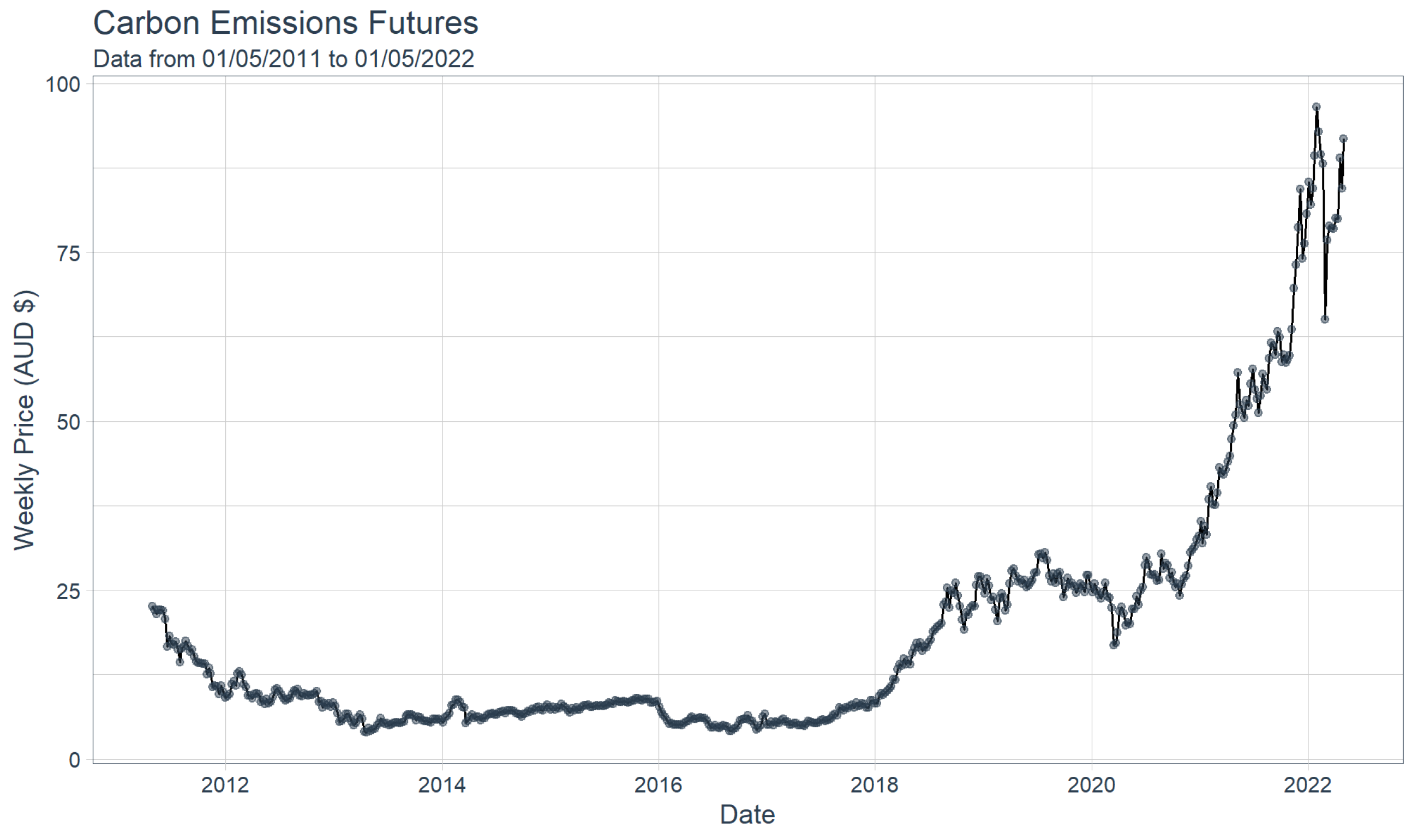
4. A Financial Time Series Modelling Application

The financial Carbon Emissions Futures price between the dates of 1 May 2012 and 1 May 2022 which is shown at Figure 6, has been modelled using the Box–Jenkins, GBM and the Tsallis time series modelling methods. Modelling to determine the datasets distribution and undertaking simple linear regression modelling allows for a goodness-of-fit assessment between the original and generated time series models, which can serve as a criterion for model selection.

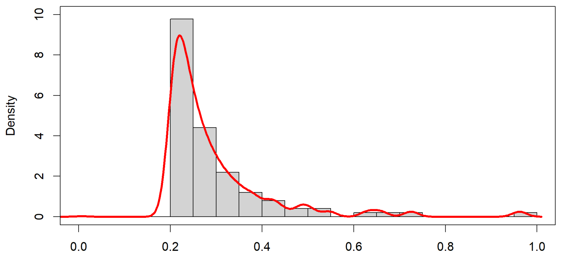
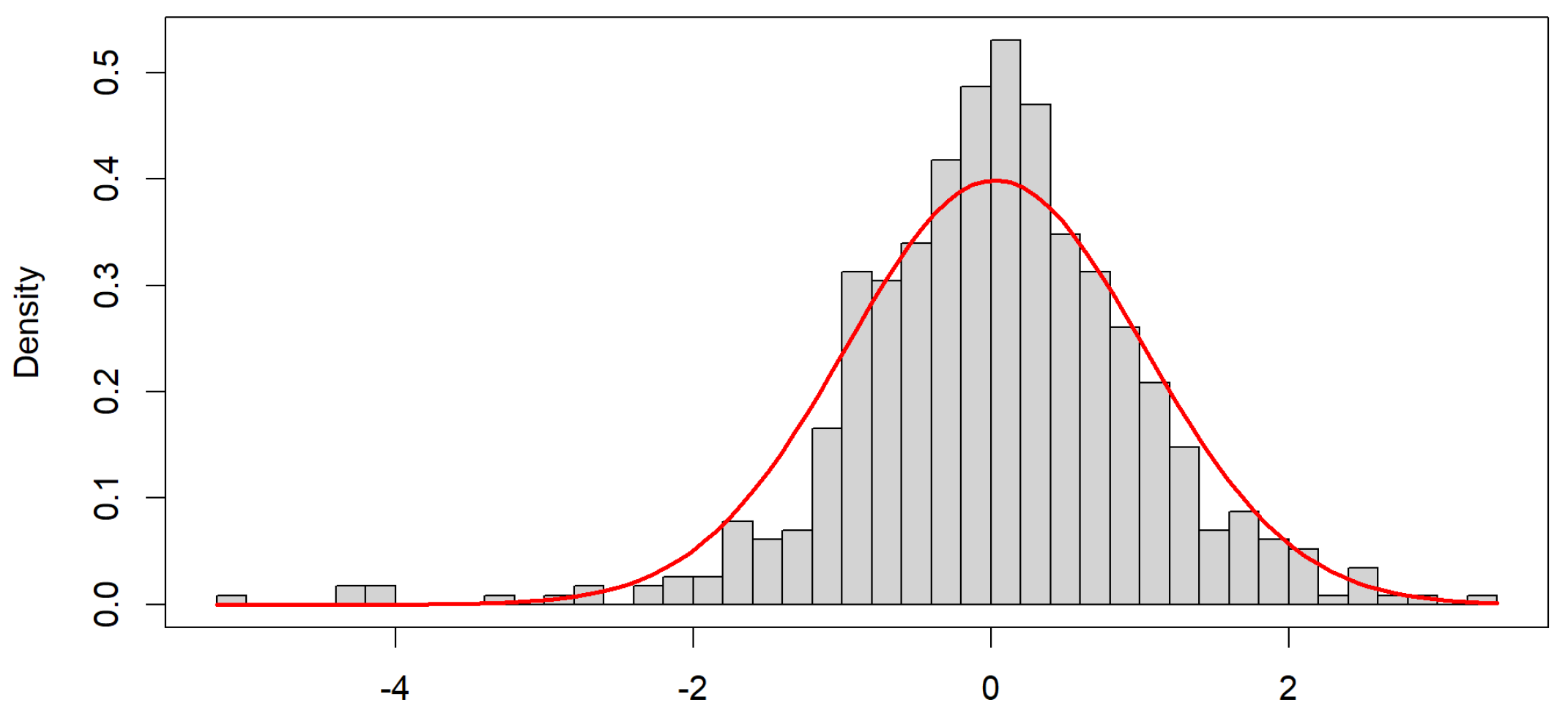
4.1. Determining the Initial Distribution

Determining the time series distribution was undertaken using the Box-Jenkins methodology to stabilize the time series dataset, see Figure 7. The resulting distribution of the log-differenced residual distribution at Figure 8, shows that the residuals are normal slightly skewed with a long thin tail. The log-differenced results of the Carbon Emissions price distribution at

Table 1. Modelling Results.

Model	$\widehat{\mathit{\mu }}$	$\widehat{\mathit{\sigma }}$	Intercept	Slope	Std Error	${\mathit{R}}^2$	p-Value	AIC	BIC
Log-diff.	0.002	0.068	−0.011	0.000	0.068	0.011	0.007	−1457.4	−1444.4
ARIMA	0.000	0.084	0.000	0.000	0.084	−0.002	0.986	−1206.6	−1193.6
SGARCH	0.061	0.999	−0.156	0.001	0.993	0.014	0.003	1627.4	1640.4
TGARCH	0.026	1.000	−0.237	0.001	0.990	0.021	0.000	1624.3	1637.4
GJR-GARCH	0.057	1.036	−0.323	0.001	1.013	0.043	0.000	1651.1	1664.1
GBM	0.002	0.068	−0.006	0.000	0.063	0.011	0.011	−1532.1	−1519.0
Tsallis	0.033	0.806	−0.452	0.000	0.890	0.001	0.644	725.8	736.6

, produced a mean $\widehat{\mu }=0.0024$ and the standard deviation $\widehat{\sigma }=0.0681$ indicates a low level of dispersion. The kurtosis of the distribution suggests that low values of the Carbon price resulted in volatility, see Figure 8 and Figure 9.

The distribution at Figure 8, is the time series distribution for the Carbon price. Further modelling is required in constructing a mathematical model that will allow for forecasting. The distribution at Figure 8, can be used within a bivariate regression model, Liu et al. (2020) and/or a bivariate copula model, Dewick and Liu (2022) if required.

Regression modelling has been used as a methodology in determining a suitable distribution that represents the initial distribution, see Figure 8 which can be used in model selection. The regression model for the initial distribution is shown at Figure 10, with the results shown at Table 1. This allows the initial distribution to be used as a baseline in comparing other distributions produced from using the Box-Jenkins, Geometric Brownian Motion and Tsallis methods.

4.2. Box–Jenkins Time Series Modelling Methodology

The Autocorrelation Function (ACF) and the Partial Autocorrelation Function (PACF) plots identified at Figure 11, shows that there is a persistence of volatility, therefore a GARCH type model is required.

Initial ARIMA modelling of the dataset at Figure 6, was undertaken using the R package function auto.arima and gave the best fitting model as: ARIMA$(1,2,0)$. Further modelling was undertaken using the R package function rugarch. This package produced the best fitting models as: SGARCH$(1,0,2)(2,1)$, TGARCH$(1,0,2)(1,1)$ and the GJR-GARCH$(1,0,2)(2,1)$. These models were modeled for their distributions and regression modelling was undertaken. The TGARCH model residuals and Q-Q plot is shown at Figure 12 and Figure 13. Further GARCH type models could also have been used but this paper has used the ones shown as examples.

Simple linear regression modelling using the original and TGARCH distributions, see Equation (1), are shown at Figure 10 and Figure 14. The results for all the modelled distributions using simple linear regression undertaken are given at Table 1.

Overall, the results show that the time series distribution is symmetric. The lower tail being thin, suggests that the skew represents rare events. This is highlighted in comparing the Q-Q plots similarities at Figure 9 and Figure 13.

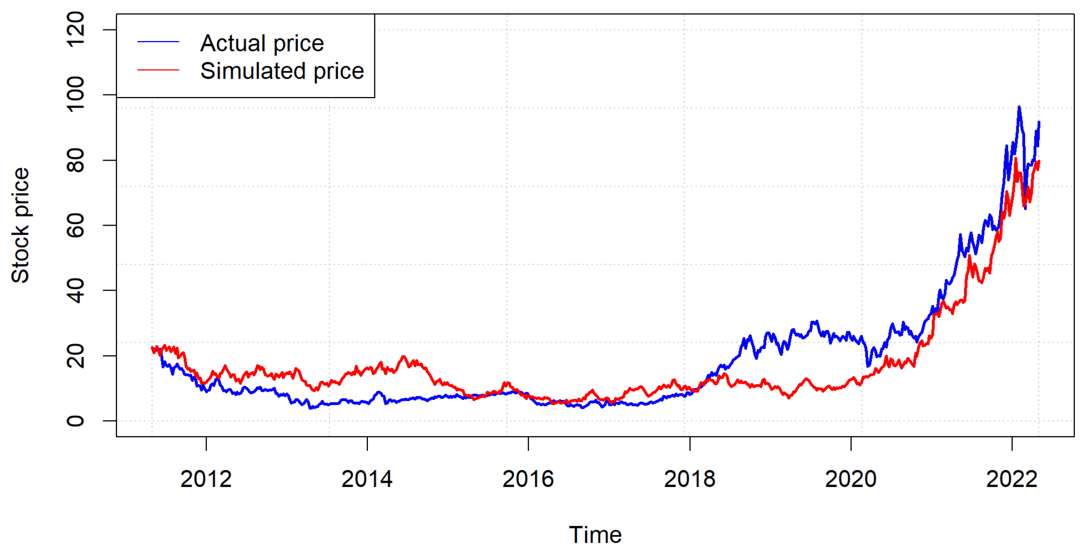
4.3. Time Series Brownian Motion Results

A Time Series Geometric Brownian Motion simulation was undertaken with input parameters for the GBM being identified using the initial Box-Jenkins model results $(\widehat{\mu }=0.0024,\widehat{\sigma }=0.0681)$, shown at Figure 8. To allow for the simulation to represent the dataset, hundreds of simulations Khamis et al. (2017), may be required. GBM simulations tend to fluctuate wildly, this is highlighted at Figure 15, as 518 simulations were required to produce the better fitting model which is shown at Figure 16.

The Geometric Brownian Motion model required the distribution required to be log-differenced to stabilize the data using the same methodology shown at Figure 7 and Figure 8. The simple linear regression modelling results for the Geometric Brownian Motion are given at Table 1.

4.4. Tsallis Entropy Results

A Tsallis entropy estimation was undertaken using the R package q-Gaussian, de Santa Helena and de Lim (2018). This R package allows for the calculation of the Tsallis q value in determining the q-Gaussian distribution see Figure 2, that would indicate if the time series distribution contained fat or thin tails. The simple linear regression model for the Tsallis modelling results is at Table 1.

The R package tsallisexp is a package that can be used to determine the quality of fit to an exponential distribution, as $q\to 1$, an exponential distribution is obtained, Shalizi and Dutang (2021). Due to the small dataset size 575 data points, far less than what is required, ${10}^6$ data points. Entropy Modelling is a methodology that can be easily undertaken should a large enough dataset be available.

5. Modelling Results Summary

Simple linear regression was undertaken on the resulting distributions shown at Table 1. The results show the GBM model, Figure 16 gave the best modelling results that matched the original log-differenced dataset. The results also shows that modelling using the GARCH family, the TGARCH model bests goodness-of-fit with the original log-differenced dataset as there is slight volatility. This slight volatility (skew) was highlighted within the original distribution at Figure 8 and Figure 9.

6. Conclusions

This study has modelled time series data using three different modelling methods in identifying the underlying distribution that can result due to the different phenomenon that affect the financial market. The purpose and utility of determining the underlying distribution is three-fold, firstly, these distributions can be used with regression modelling as a goodness-of-fit criterion when undertaking forecasting modelling. Secondly, the distribution can be applied in other modelling methods, such as regression and copula modelling. Thirdly, by understanding the initial distribution of the dataset will give insight to the possible presents of volatility (and leverage affects) and drift that can result from different phenomenon’s acting within the financial market.

Using Tsallis entropy for time series modelling could be a good option in determining the distribution, however it does require a large dataset (${10}^6$), which may not be practically available. This study used Tsallis Entropy modelling in determining the q-Gaussian distribution, but it failed to reproduce the valid results. It is unsure how small a dataset could be to produce a q-Gaussian distribution with reasonable accuracy in determining the underlying distribution using this application, this could be a topic for further research. In an environment using Big-Data, Tsallis entropy could be a quick methodology in identifying the underlying distribution.

Future applications may include that time series modelling, not just be focused on determining a predictive forecasting model, but rather being more focused on determining and identifying the underlying distribution and parameters which aids in model selection by using regression methods, then proceed to either other modelling methods, such as regression, copula modelling or to forecasting methods and methodologies.

Limitations of this study is that only a few GARCH type models were used, being the SGARCH, TGARCH and GJR-GARCH type models. This study has highlighted that there are many GARCH type models that can be used. Familiarity for all the GARCH type models should be obtained that will allow for the modelling the stylized facts from the time series distribution.

References

1. Abdulla, Suhail Najm, and Heba Dhaher Alwan. 2022. Using apgarch/avgarch models Gaussian and non-Gaussian for modeling volatility exchange rate. International Journal of Nonlinear Analysis and Applications 13: 3029–38. [Google Scholar]
2. Afuecheta, Emmanuel, Artur Semeyutin, Stephen Chan, Saralees Nadarajah, and Diego Andrés Pérez Ruiz. 2020. Compound distributions for financial returns. PLoS ONE 15: e0239652. [Google Scholar] [CrossRef] [PubMed]
3. Agustini, W. Farida, Ika Restu Affianti, and Endah R. M. Putri. 2018. Stock price prediction using geometric Brownian motion. Journal of Physics: Conference Series 974: 012047. [Google Scholar]
4. Bentes, Sónia R., Rui Menezes, and Diana A. Mendes. 2008. Stock market volatility: An approach based on Tsallis entropy. arXiv arXiv:0809.4570. [Google Scholar]
5. Bollerslev, Tim. 1986. Generalized autoregressive conditional heteroskedasticity. Journal of Econometrics 31: 307–27. [Google Scholar] [CrossRef] [Green Version]
6. Caporin, Massimiliano, and Michele Costola. 2019. Asymmetry and leverage in GARCH models: A news impact curve perspective. Applied Economics 51: 3345–64. [Google Scholar] [CrossRef] [Green Version]
7. Charles, Amélie, and Olivier Darné. 2019. The accuracy of asymmetric GARCH model estimation. International Economics 157: 179–202. [Google Scholar] [CrossRef]
8. Charpentire, Arthur. 2014. Computational Actuarial Science with R. New York: CRC Press. [Google Scholar]
9. de Santa Helena, Emerson Luis, C. M. Nascimento, and G. Gerhardt. 2015. Alternative way to characterize a q-Gaussian distribution by a robust heavy tail measurement. Physica A: Statistical Mechanics and Its Applications 435: 44–50. [Google Scholar] [CrossRef] [Green Version]
10. de Santa Helena, Emerson Luis, and Wagner Santos de Lima. 2018. Package ‘qGaussian’. R Package Version 0.1.8. Available online: https://CRAN.R-project.org/package=qGaussian (accessed on 24 April 2022).
11. Devi, Sandhya. 2021. Asymmetric Tsallis distributions for modeling financial market dynamics. Physica A: Statistical Mechanics and Its Applications 578: 126109. [Google Scholar] [CrossRef]
12. Dewick, Paul R., and Liu Shuangzhe. 2022. Copula modelling to analyse financial data. Journal of Risk and Financial Management 15: 104. [Google Scholar] [CrossRef]
13. Ermogenous, Angeliki. 2006. Brownian Motion and Its Applications in the Stock Market. Available online: https://ecommons.udayton.edu/cgi/viewcontent.cgi?article=1010&context=mth_epumd (accessed on 12 May 2022).
14. Fukuda, Kosei. 2021. Selecting from among 12 alternative distributions of financial data. Communications in Statistics-Simulation and Computation 51: 3943–3954. [Google Scholar] [CrossRef]
15. Ghani, I. M. Md, and H. A. Rahim. 2019. Modeling and forecasting of volatility using arma-garch: Case study on malaysia natural rubber prices. IOP Conference Series: Materials Science and Engineering 548: 012023. [Google Scholar] [CrossRef]
16. Hambuckers, Julien, and Cedric Heuchenne. 2017. A robust statistical approach to select adequate error distributions for financial returns. Journal of Applied Statistics 44: 137–61. [Google Scholar] [CrossRef]
17. Heyde, C. Heyde, and Shuangzhe Liu. 2001. Empirical Realities for Minimal Description Risky Asset Model. The Need for Fractal Features. Journal of the Korean Mathematical Society 38: 1047–59. [Google Scholar]
18. Heyde, C. Heyde, Roger Gay, and Shuangzhe Liu. 2001. Fractal scaling and Black-Scholes [A new view of long-range dependence in stock prices]. JASSA 1: 29–32. [Google Scholar]
19. Hongwiengjan, Warunya, and Dawud Thongtha. 2021. An analytical approximation of option prices via TGARCH model. Economic Research-Ekonomska Istraživanja 34: 948–69. [Google Scholar] [CrossRef]
20. Islam, Mohammad Rafiqul, and Nguyet Nguyen. 2021. Comparison of Financial Models for Stock Price Prediction. Joint Mathematics Meetings (JMM) 13: 181. [Google Scholar] [CrossRef]
21. Kapusta, Joseph I. 2021. Perspective on Tsallis statistics for nuclear and particle physics. International Journal of Modern Physics E 30: 2130006. [Google Scholar] [CrossRef]
22. Khamis, Azme, M. A. A. Sukor, M. E. Nor, S. N. A. M. Razali, and R. M. Salleh. 2017. Modeling and Forecasting Volatility of Financial Data using Geometric Brownian Motion. International Journal of Advanced Research in Science, Engineering and Technology 4: 4599–605. [Google Scholar]
23. Lim, Ching Mun, and Siok Kun Sek. 2013. Comparing the performances of GARCH-type models in capturing the stock market volatility in Malaysia. Procedia Economics and Finance 5: 478–87. [Google Scholar] [CrossRef] [Green Version]
24. Liu, Shuangzhe, and Chris C. Heyde. 2008. On estimation in conditional heteroskedastic time series models under non-normal distributions. Statistical Papers 49: 455–69. [Google Scholar] [CrossRef]
25. Liu, Timina, Shuangzhe Liu, and Lei Shi. 2020. Time Series Analysis Using SAS Enterprise Guide. Singapore: Springer Nature. [Google Scholar]
26. Oliveira, Gustavo H. F. M., Rodolfo C. Cavalcante, George G. Cabral, Leandro L. Minku, and Adriano L. I. Oliveira. 2017. Time series forecasting in the presence of concept drift: A pso-based approach. Paper presented at the 2017 IEEE 29th International Conference on Tools with Artificial Intelligence ICTAI), Boston, MA, USA, November 6–8; pp. 239–46. [Google Scholar]
27. Pavlos, G. P., L. P. Karakatsanis, M. N. Xenakis, E. G. Pavlos, A. C. Iliopoulos, and D. V. Sarafopoulos. 2014. Universality of non-extensive Tsallis statistics and time series analysis: Theory and applications. Physica A: Statistical Mechanics and Its Applications 395: 58–95. [Google Scholar] [CrossRef]
28. Sato, Aki-Hiro. 2010. q-Gaussian distributions and multiplicative stochastic processes for analysis of multiple financial time series. Journal of Physics: Conference Series 201: 012008. [Google Scholar] [CrossRef]
29. Shalizi, Cosma, and Christophe Dutang. 2021. tsallisqexp: Tsallis Distribution. R Package Version 0.9-4. Available online: https://CRAN.R-project.org/package=tsallisqexp (accessed on 15 May 2020).
30. Sheraz, Muhammad, and Imran Nasir. 2021. Information-Theoretic Measures and Modeling Stock Market Volatility: A Comparative Approach. Risks 9: 89. [Google Scholar] [CrossRef]
31. Stoyanov, Stoyan V., Svetlozar T. Rachev, Boryana Racheva-Yotova, and Frank J. Fabozzi. 2011. Fat-tailed models for risk estimation. The Journal of Portfolio Management 37: 107–17. [Google Scholar] [CrossRef] [Green Version]
32. Teräsvirta, Timo. 2009. An introduction to univariate GARCH models. In Handbook of Financial Time Series. Berlin and Heidelberg: Springer, pp. 17–42. [Google Scholar]
33. Tsallis, Constantino. 2017. Economics and Finance: q-Statistical stylized features galore. Entropy 19: 457. [Google Scholar] [CrossRef]
34. Wheelwright, Steven, Spyros Makridakis, and Rob J. Hyndman. 1998. Forecasting: Methods and Applications. Hoboken: John Wiley & Sons. [Google Scholar]
Figure 1. Normal and Student-t Distributions.
Jrfm 15 00461 g001
Figure 2. q−Gaussian Distributions.
Jrfm 15 00461 g002
Figure 3. Skewed Student-t Distribution.
Jrfm 15 00461 g003
Figure 4. Generalized Error Distribution.
Jrfm 15 00461 g004
Figure 5. Pareto Distribution.
Jrfm 15 00461 g005
Figure 6. Time Series Plot.
Jrfm 15 00461 g006
Figure 7. Log−Differenced Residuals.
Jrfm 15 00461 g007
Figure 8. Log−Differenced Residual Distribution.
Jrfm 15 00461 g008
Figure 9. Log−Differenced Residual Q-Q Plot.
Jrfm 15 00461 g009
Figure 10. Regression Plot for the Log−Differenced Residual Distribution.
Jrfm 15 00461 g010
Figure 11. ACF and PACF of the Log−Differenced Carbon Emissions Dataset.
Jrfm 15 00461 g011
Figure 12. TGARCH Model Residual Distribution.
Jrfm 15 00461 g012
Figure 13. TGARCH Residual Distribution Q−Q Plot.
Jrfm 15 00461 g013
Figure 14. Regression Plot for the TGARCH Residual Distribution.
Jrfm 15 00461 g014
Figure 15. GBM Simulation No.105.
Jrfm 15 00461 g015
Figure 16. GBM Simulation No.518.
Jrfm 15 00461 g016