Factor-Based Investing in Market Cycles: Fama–French Five-Factor Model of Market Interest Rate and Market Sentiment

Abstract

This study explores risk–reward patterns in the US stock market and establishes optimal factor-based investing using the Fama–French five-factor model through market cycles constructed by Shiller’s interest rates and Baker–Wurgler’s sentiments. Our emerging evidence confirms that the high-interest rate, high-sentiment cycle generates higher excess returns, and the low-interest rate, low-sentiment cycle generates lower excess returns, which supports the hypothesis that the market cycles as investment horizons have an asymmetric effect on stock returns. Furthermore, the size factor outperforms in the low-interest rate, low-sentiment cycle, whilst the value factor outperforms in the high-interest rate, high-sentiment cycle. Using the asymmetric GARCH model, the asymmetric leverage effect of interest rates and sentiments on five-factor returns is empirically demonstrated with explanatory power of five-factor characteristics. Unlike previous studies, our findings also imply that high- and low-sentiment cycles asymmetrically affect the value factor, and the value premium does not disappear over time, highlighting the role of the market cycles in five-factor returns.

1. Introduction

Would we recommend the five-factor model in applications? Factor models are often used to evaluate portfolio performance—Fama and French (2017). The risk–return trade-off in traditional financial theory advocates for a diversified strategy to decrease the volatility of investment portfolios and optimise returns. The literature discusses three sources of returns in asset pricing: market risk premium, factor premium, and excess return or alpha. Investment practice claims that, in the long term, actively managed funds outperform the market; however, empirical evidence for the alpha remains weak (Blitz 2015). Therefore, investors increasingly rely on passive value-weighted market indexes at the lowest cost. Whilst passive investing can capture market risk premium, this approach risks missing the factor premium.

Factor-based investing is a strategy in which securities are chosen according to the attributes of higher returns based on macroeconomic and style factors—the former covers the systematic risks of asset classes and the latter explains the risk–return relationship of risk factors. Fama and French (1993) developed a three-factor model that includes market, size, and value factors to explain the cross-sectional stock returns, thus setting the benchmark for multi-factor models. Carhart (1997) proposed a four-factor model, comprising three factors plus the momentum factor, to supplement the anomalies that the three-factor model could not capture. With the expansion of factor theory, Novy-Marx (2013) introduced the profitability factor. Subsequently, Fama and French (2015) established the five-factor model (FF5), adding profitability and investment factors to the three-factor model. The FF5 model broadly explains the patterns in average returns for the pricing ability of risk factors.

An authentic risk factor must be able to predict the future expected return or fluctuation to prove its risk premium’s rationality in an equilibrium state. Harvey et al. (2015) surveyed 316 factors and reported that some are related to macroeconomic variables, others are interpreted as either risks or behavioural biases, and yet other factors are liable to both risks and behavioural biases. Daniel and Titman (1998) found that the performance of the characteristics model (non-risk-based) is superior to that of the covariances model (risk-based) in predicting the expected returns of the stock market. Recent studies argue that most factors are subject to factor decay or are affected by data snooping, investor behaviour, or randomness without the robustness of the factor premium.

Research demonstrates the long-term correlation between factor premiums and economic cycles in the US stock market. The value premium has a comparable negative correlation with monetary policy (Black et al. 2009), and the performance of small-cap stocks is more cyclical than that of large-cap stocks (Yogo 2006). The negative value premium (−5.4%) from 2007 to 2020 occurred due to changes in the economic structure and long-term low-interest rates (Arnott et al. 2021). In other words, the size and value factors do not always exist, and even appear to be in a reverse relationship in some periods (Hirshleifer 2001). As the factor premium has economic cyclicity, different factors have a similar dependency on macroeconomics. Even amongst factors with low correlation, a multi-factor portfolio may not be able to avoid macroeconomic risks (Amenc et al. 2019). In this regard, Campbell (1987) evinces the effectiveness of the term structure of interest rates in predicting excess returns in the US stock market. Empirically, the fluctuation of interest rates and stock prices shows a reverse trend with a time lag, where returns on common stock are related to the change in the interest rate (Flannery and James 1984).

In addition, volatility is an important component of asset pricing, and investors are considered to be rational in conventional financial theory. However, an overview of the financial crises that occurred over past years shows that investor sentiment causes fluctuations in stock prices, which deviate from their intrinsic values (De Bondt and Thaler 1985; Brown and Cliff 2004). The excessive optimism (pessimism) of investors causes stock prices to be overvalued (undervalued). In short, investor sentiment influences the performance of stock prices (Baker and Stein 2004). Rupande et al. (2019) evinced a significant connection between investor sentiment and stock return volatility using the generalised autoregressive conditional heteroscedasticity (GARCH) model. Gregoriou et al. (2019) demonstrated a seven-factor asset pricing model, where they merge insights from Expected Utility Theory and Prospect Theory attempting to thoroughly explain changes in asset returns.

Whether the key factor affecting anomalies in stock returns is the fundamental risk or sentiment risk remains to be explored in more literature. In view of the past research on factor-based investing, factor spanning tests almost served as the verification of long-term performance, whereas market cycles related to macroeconomics and investor behaviour have not been simultaneously considered. Motivated by the FF5 model and inspired by behavioural finance, we conjecture that interest rates and sentiments may drive the risk–reward pattern of the financial market. Hence, we comprehensively employ the market cycle constructed by market interest rates and market sentiments to verify the five-factor returns and characteristics for the US stock market.

Our research deals with the following subjects: (a) identifying the critical factors influencing returns and volatility through the FF5 model; (b) inferring that interest rate cycles and sentiment cycles have an asymmetric effect on five-factor returns; and (c) assessing the performance of the FF5 model in relation to economic regimes, as generated by market cycles, to obtain optimal factor returns. We contribute to the corpus of literature on factor-based investing in three ways: we examine the risk–reward pattern of the FF5 model using the asymmetric GARCH model; our results support the hypotheses that interest rates and sentiments sufficiently expound an asymmetric effect on stock returns and five-factor returns; and we provide a brand-new investment horizon to investigate the optimal factors in each market cycle as factor investing strategies.

The rest of the paper is organised as follows. Section 2 reviews the relevant literature on factor-based investing and market cycles. Section 3 defines the data and methodology. Section 4 delivers empirical results. Section 5 offers an extended discussion. Section 6 refers to the robustness test with alternative variables. Section 7 concludes.

2. Literature Review

2.1. Factor-Based Investing

The pioneering study of Arnott et al. (2005) inspired the conceptualisation of factor-based investing. Investors tend to group securities according to certain characteristics, such as size, book-to-market ratio, and past performance, and select specific stocks to invest in. Virtually, style-rotating strategies can generate superior returns (Asness et al. 2000; Lucas et al. 2002). Barberis and Shleifer (2003) proposed a style-investing model for asset allocation based on two premises: first, funds will move towards the style with relatively better performance in the past (positive feedback trading); second, the flow of funds will affect the relative prices of style investing.

Blitz et al. (2014) recommend that investors strategically allocate the factor premium, in addition to the risk premium provided by conventional asset classes. Dimson et al. (2017) investigated the growth and risk–return relationship of exchange-traded funds and exchange-traded products based on smart beta strategies. In addition to the Fama–French five-factor and the momentum factor of Jegadeesh and Titman (1993), Asness et al. (2015) proposed four typical styles of factor premia: value, momentum, carry, and low volatility factor. Ang et al. (2018) found that factor portfolios of value, size, momentum, profitability, and low volatility stocks historically provide higher risk-adjusted returns. Behavioural finance shifts the focus from risk factors to investor behaviour. In particular, the effect of mispricing caused by overconfidence is more likely to occur in growth stocks (Daniel and Titman 1998). Lee and Swaminathan (2000) proposed a momentum lifecycle model that shows underreaction and overreaction of shocks to stock prices, forming a style rotation of value and growth stocks.

In modern portfolio theory, using the low (negative) correlation between factors can reduce the overall portfolio’s volatility, thereby optimising risk-adjusted returns. However, the empirical results may vary across sample periods regardless of whether the FF5 or multi-factor model is used. The differences may be attributed to the evolution of the market structure, interpretation in terms of risk or behaviour, and the effect of economic regimes.

2.2. Five-Factor Model

Fama and French (2015) suggested using profitability and investment factors, in addition to existing factors (market, size, and value) in the three-factor model, to capture patterns in average stock returns. The FF5 model explains the relationship between the five-factor and portfolio expected returns from the dividend discount model perspective and the valuation theory. In the FF5 model, Ri, Rf, and Rm are the expected return, risk-free rate, and market return, respectively. SMB, HML, RMW, and CMA are the risk premium factors, denoting the size, value, profitability, and investment factor, respectively. The fundamental model of FF5 is expressed as follows:

Ri_t − Rf_t = α + β_market(Rm_t − Rf_t) + β_sizeSMB_t + β_valueHML_t + β_{profitability}RMW_t + β_investmentCMA_t + ε_t

2.2.1. Size Factor

Banz (1981) found that small-cap stocks outperform large-cap stocks, regardless of the market beta value. Nevertheless, Horowitz et al. (2000) argued that there is no visible evidence of the small-cap effect in the US stock market from 1980 to 1996. Indeed, institutional investors have preferred large-cap stocks over the past 20 years. The change in demand for competitive styles could be the cause of the relatively poor performance of small-cap stocks (Gompers and Metrick 2001). Although risk can explain the size premium, in behavioural finance, the anomaly of small-cap growth stocks is considered to be evoked by investors’ lottery-like (positively skewed) preferences (Barberis and Huang 2008). Noticeably, when testing on international markets, the FF5 model does not fully capture the low average returns on the small-cap stocks of low-profit companies with aggressive investments. From 1990 to 2015, the size factor seems redundant in major markets outside the North America region (Fama and French 2017).

2.2.2. Value Factor

The value premium is important for long-term factor investing portfolios. Asness et al. (2013) investigated the stock markets of 18 developed countries and found universal evidence of the value premium. Zhang (2005) argued that the value premium may represent the asymmetric risk of value stocks in accordance with economic regimes. The interpretation of the value premium based on behavioural finance comes from mispricing. Investors are generally optimistic about growth stocks and overly pessimistic about value stocks (Lakonishok et al. 1994). Interestingly, Fama and French (2015) concluded that the value factor is redundant in describing the average return on the US stock market (1963–2013). The other four factors fully explain the average return because the positive intercept of the value factor from 1963 to 1989 is offset by its negative intercept in the subsequent period (1990–2013).

2.2.3. Profitability Factor

Fama and French (2006) proved that, after controlling for the book-to-market ratio and investment factor, companies with large profit margins yield higher returns. By examining cross-sectional stock returns, Novy-Marx (2013) found that predicted average returns based on profitability are similar to the results based on the book-to-market ratio. The profitability factor is the most useful tool for predicting low volatility (Novy-Marx and Velikov 2016). From the viewpoint of behaviour finance, investors are overly optimistic about the mean reversion of unprofitable companies, which contributes to the overvaluation of their stocks. In addition to the mispricing of unprofitable companies with high information uncertainty, arbitrage difficulty and financial distress can also generate the profitability premium (Liu 2015).

2.2.4. Investment Factor

As the global version of the three-factor model cannot explain regional expected returns, the FF5 model can more efficiently interpret the return pattern of equilibrium asset pricing (Ryan et al. 2021). The positive slope of the profitability and investment factors (conservative investment in profitable companies) yields a higher average return with a lower market beta. Conversely, the negative slopes of profitability and investment factors (aggressive investment in unprofitable companies) exhibit a lower average return with a higher market beta. The explanatory power of the FF5 model corresponds to the slopes of the profitability and investment factors. Empirically, the investment factor contributes to explaining regional abnormal returns in North America and the Asia-Pacific region but seems redundant for Europe and Japan (Fama and French 2017).

2.3. Market Cycles

From the mid-1970s to the 1980s and the early 2000s, the performance of the profitability factor was relatively poor, whereas the yields of the value factor underperformed in the 1990s and 2010s. Simply, when the performance of the value strategy worsens, the growth strategy based on the profitability factor improves, and vice versa. From 2010 to 2019, except for the high excess returns of the market premium, the aggregate returns of the other four factors approached zero, similar to 1990–1999 (Blitz 2020). The average return of the value factor was particularly poor in this period. Israel et al. (2021) and Fama and French (2021) attempted to reinterpret the disappearance of the value premium—is it possible for factor decay of the value factor to occur?

Factor premium is inseparable from macroeconomic factors. Peng and Zervou (2022) indicated that monetary policy objectives play an essential role in affecting risk sharing, asset returns, and equity premiums. As monetary policy determines the interest rate level, stock returns during periods of monetary easing are regularly higher than during periods of tight monetary policy (Jensen and Johnson 1995). Interest rates reflect the overall trend of alternating expansion and contraction of economic cycles with short- and long-term effects on the stock market. Compared with short-term interest rates, long-term interest rates are more closely affiliated with stock returns (Abdullah and Hayworth 1993). Baks and Kramer (1999) studied the mechanism of currency liquidity in the international market and found that an increase in money liquidity is consistent with the decline in real interest rates and the rise in stock prices.

Furthermore, investor sentiment may affect the security prices in the same direction at the same time (Stambaugh et al. 2012). Stock markets will yield a relatively higher (lower) return following low (high) sentiment (Baker and Wurgler 2006). Following high and low sentiment periods, the market and size factors present more obvious influences; conversely, the value factor does not exhibit a significant difference (Stambaugh et al. 2012). Surveying the consumer confidence index, Schmeling (2009) found that consumer sentiment in various countries has a negative correlation with stock returns, which is also applicable to the reward patterns of value, growth, and small-cap stocks.

In general, the above literature shows that the market interest rate indirectly affects the money supply, and stock prices move inversely to the trend of interest rates. Market sentiment stems directly from investors’ optimistic or pessimistic behaviour on the stock market. The portfolio return seems to be exposed to specific risk and behaviour factors—a factor that is redundant in one economic cycle may be consequential in another. Thus, we construct market cycles by synthesising the macroeconomic variable (namely, interest rate cycles) and investor behaviour variable (namely, sentiment cycles) to verify our inferences. Referring to the literature, we formulate the following hypotheses:

Hypothesis 1 (H1).

Interest rate cycles and sentiment cycles have an asymmetric effect on stock returns.

Hypothesis 2 (H2).

Market cycles have an asymmetric effect on five-factor adjusted stock returns, particularly in periods of the high-interest rate, high-sentiment cycle, and the low-interest rate, low-sentiment cycle.

3. Data and Methodology

3.1. Data

As the timeframe of the database for the three variables (market interest rate, market sentiment, and five-factor returns) in this study is not synchronised, the sample period of empirical analysis proceeds through the intersection period of three variables with 642 monthly observations stretching from July 1965 to December 2018.

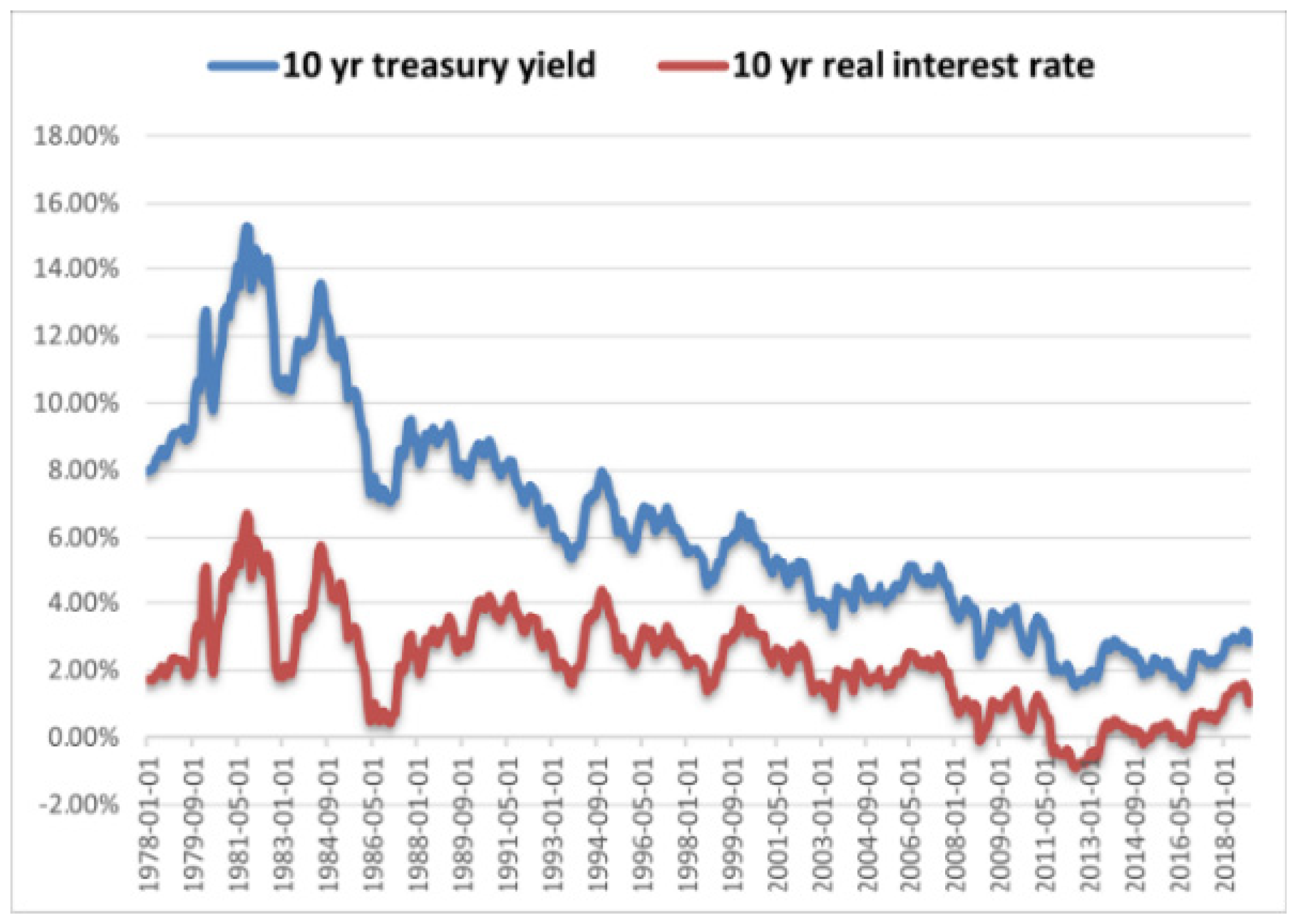
3.1.1. Market Interest Rate

Campbell and Shiller (1988) indicated that, in asset pricing, the discount rate stands for the capitalisation of dividends, or equity financing costs should be the real interest rate, not the nominal interest rate. Campbell and Shiller (1998) found that the real excess return on stocks relative to bonds is affected by the cyclically adjusted price-to-earnings ratio (CAPE). Subsequently, Shiller et al. (2020) surveyed the effect of the COVID-19 pandemic on the stock markets of five major economies and found that the CAPE does not consider the interest rate effect on the market. Hence, the excess CAPE yield (ECY) is proposed as a measure of the equity risk premium. Shiller et al. explained that the ECY indicator represents adjusted excess return, which can effectively evaluate the interaction between stock long-term valuation and long-term interest rate. The equation for ECY is the current reciprocal of CAPE minus the current 10-year real interest rate:

Excess CAPE yield_t = (1/CAPE_t) − 10 year interest rate_t

We adopt Shiller’s long-term real interest rate, that is, the 10-year real interest rate (variable termed RIS) as the proxy variable for the market interest rate for two reasons: first, the long-term real interest rate incorporates the effect of expected inflation on the stock market; second, the real interest rate is more likely than the nominal interest rate to respond to the economic implications of the negative interest rate policy. The long-term real interest rate data are derived from Shiller Online Data, which covers the period from January 1871 to the present.1 We calculate the long-term real interest rate by extracting the ECY indicator in the monthly database.

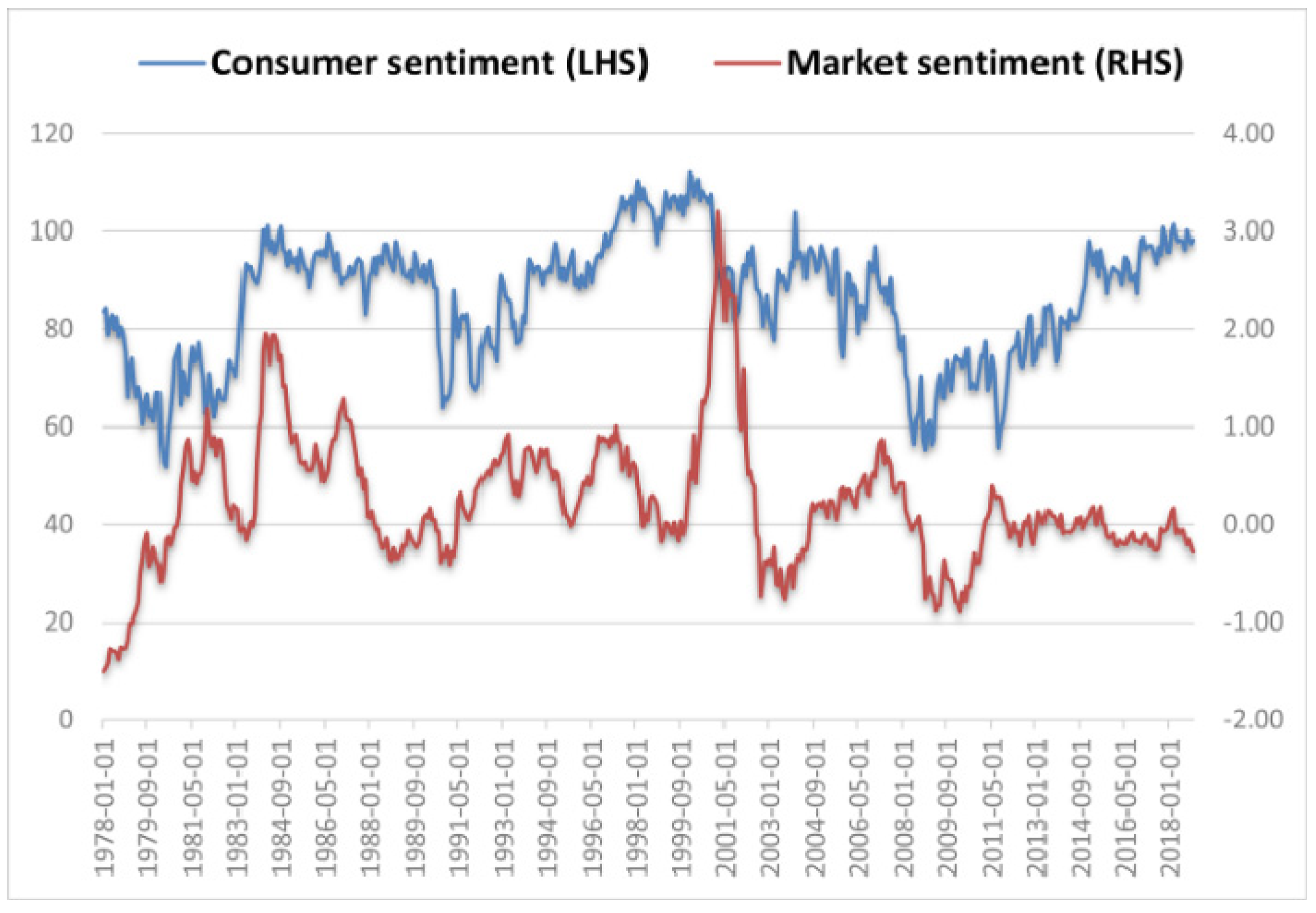
3.1.2. Market Sentiment

Many proxies are used in the literature to gauge investor sentiment. For instance, Brown and Cliff (2004) divided the measure of investor sentiment into two categories, namely, (1) direct sentiment indicators, which are usually applied by investors to conduct surveys on the public, such as the Consumer Sentiment Index of the University of Michigan; and (2) indirect sentiment indicators, where stock market information is used to capture investor sentiment. Baker and Wurgler (2006) employed six sentiment variables to extract an integrated sentiment index using principal component analysis to measure investor sentiment. Subsequently, they constructed an orthogonal sentiment index as market sentiment by regressing the six macroeconomic variables to eliminate the influence of macroeconomics on sentiment. To effectively gauge the effect of changes in market sentiment on the stock market rather than the direct sentiment of investors, we adopt Baker–Wurgler’s orthogonal sentiment indicator (variable termed STI) from Jeffrey Wurgler’s academic website as a proxy variable for market sentiment.2 The data were collected from July 1965 to December 2018.

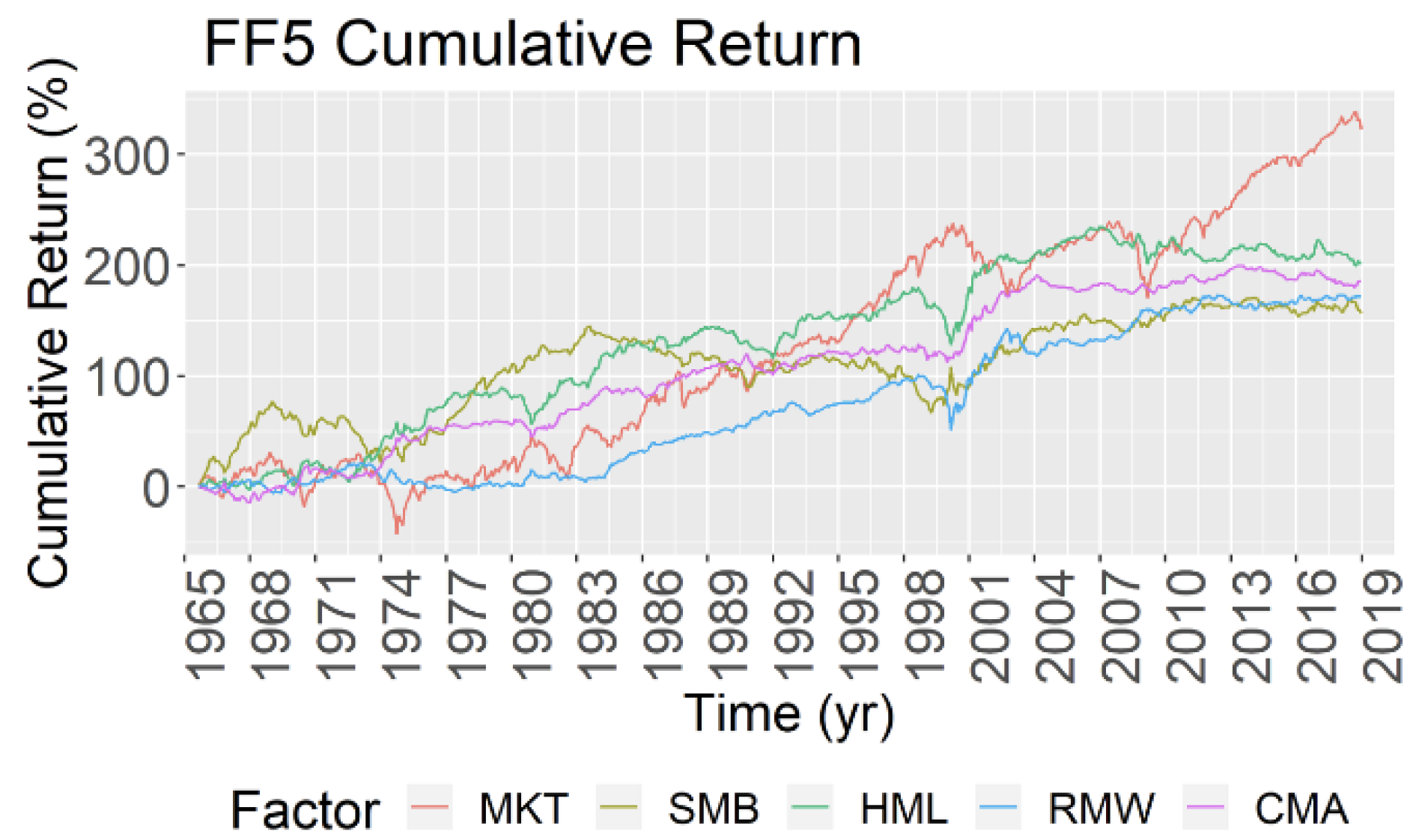
3.1.3. Five-Factor Returns

Using the Fama–French data library, we adopt the FF5 model developed by Fama and French (2015), which contains the monthly five-factor returns from July 1963 to the present.3 Additionally, the empirical analysis extracts the S&P 500 monthly price from the Compustat^® database and calculates its monthly return accordingly, which represents the monthly return of the US stock market. The variable RETURN denotes the monthly return of the S&P 500. MKT, SMB, HML, RMW, and CMA denote the monthly return of the market, size, value, profitability, and investment factors, respectively.4

Table 1. Summary statistics and correlation of the five factors.

Panel A: Summary Statistics
Factor	Mean	Std Dev	Skewness	Kurtosis	Min.	Max.	J-B p-Value
MKT	0.50%	4.46%	−0.53	4.86	−23.24%	16.10%	0 ***
SMB	0.24%	3.06%	0.36	5.94	−14.89%	18.08%	0 ***
HML	0.31%	2.84%	0.18	4.88	−11.12%	12.58%	0 ***
RMW	0.27%	2.22%	−0.36	14.91	−18.48%	13.38%	0 ***
CMA	0.29%	2.02%	0.29	4.57	−6.86%	9.56%	0 ***
Panel B: Correlation
Factor	MKT	SMB	HML	RMW	CMA
MKT	1
SMB	0.2753	1
HML	−0.2628	−0.0720	1
RMW	−0.2276	−0.3497	0.0749	1
CMA	−0.3868	−0.1094	0.6982	−0.0208	1

Note: *** denotes significance at the 1% level.

presents the summary statistics of five factors throughout the sample period. Panel A shows that the market factor averages a monthly return of 0.5%, the best amongst the five-factor returns, with the other four-factor returns ranging between 0.24% and 0.31%. The higher average monthly return of the market factor is accompanied by comparatively higher monthly volatility. Market and profitability factors are negatively skewed, whilst the other factors are positively skewed. The Jarque–Bera test rejects the assumption of the normal distribution of the five factors. Panel B shows the correlation coefficients of the five factors. Apart from the high correlation between the value and investment factors, the correlation between other factors is low overall. The market factor is positively correlated only with the size factor and negatively correlated with the other three factors.

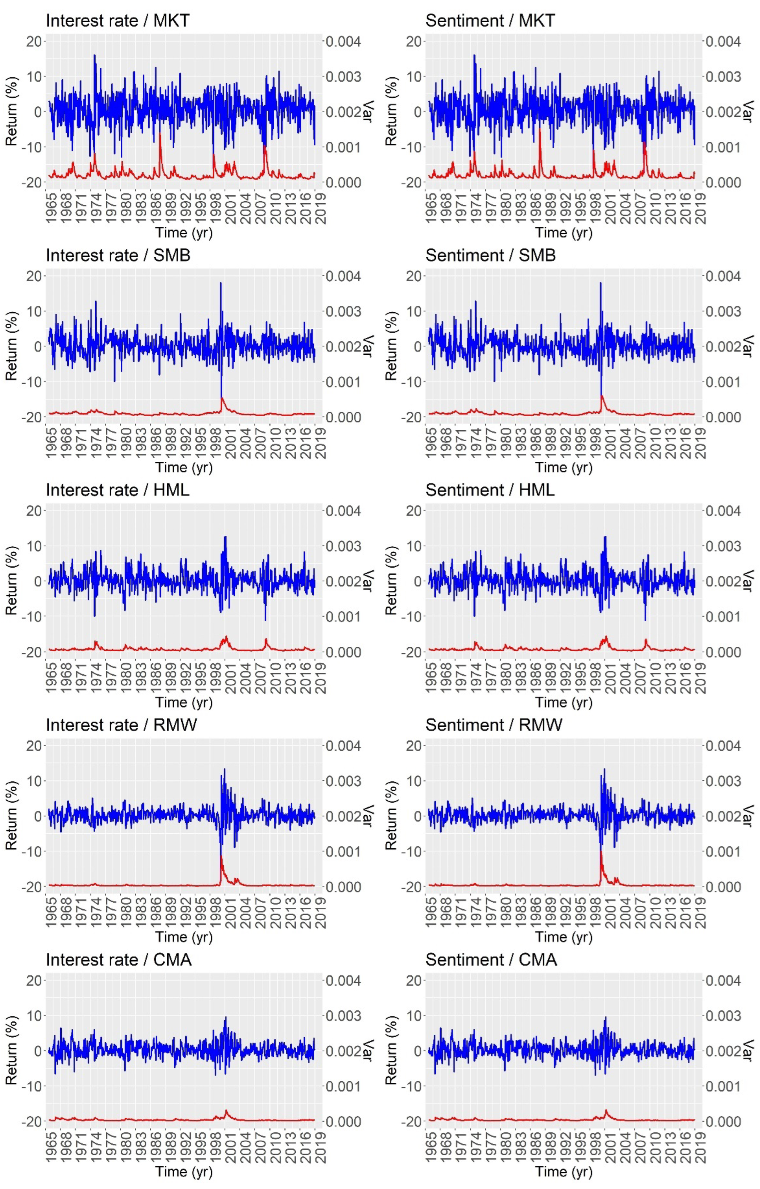
3.2. Construction of Asymmetric GARCH Model on Five-Factor Returns

Specifically, the empirical objectives of this study are to verify the asymmetric effect of interest rate and sentiment variables on the five-factor characteristics, and demonstrate the asymmetric effect of interest rate and sentiment cycles on the stock and five-factor returns.

By empirical arguments, theoretically, the five factors are convolutions of returns and time-series stationary. In the field of finance, holding risk assets often requires the risk premium, that is, the asset return is determined by risk (volatility). This model, proposed by Engle et al. (1987), is called the GARCH-in-mean model, or GARCH-M, which incorporates the GARCH variation into the mean equation.

According to Bollerslev et al. (1992), the GARCH(1,1) model can adequately capture the fluctuation process of the stock return series. Additionally, Glosten et al. (1993) modified the GARCH model to allow both positive and negative unexpected shocks to have varying influences on conditional variances, where volatility asymmetry comes from the leverage effect. Therefore, the GJR-GARCH(1,1) model is applicable for exploring the heteroscedastic variations and asymmetry in the effect of the market interest rate and market sentiment on five-factor returns.

We integrate the GJR-GARCH (1,1) and GARCH-M models into the GJR-GARCH (1,1)-M model to test whether the five factors possess a risk premium and the asymmetric effect of the rise (fall) of interest rates or sentiments in the previous period on the volatility of current five-factor returns. The empirical model is organised as follows:

R_t = α₀ + α₁ R_t−1 + θh_t + ε_t + α₂ ε_t−1, ε_t|Ω_t−1 ~ N(0, h_t),

(1)

$$h_t=c+{\beta }_0{h}_{t-1}+{\beta }_1{\epsilon }_{t-1}^2+\gamma s_{t-1}^{-}{\epsilon }_{t-1}^2+{\delta }_{1}RI{S}_{t-1}+{\delta }_{2}D RI{S}_{t-1},$$

(2)

$$h_t=c+{\beta }_0{h}_{t-1}+{\beta }_1{\epsilon }_{t-1}^2+\gamma s_{t-1}^{-}{\epsilon }_{t-1}^2+{\delta }_{1}ST{I}_{t-1}+{\delta }_{2}D ST{I}_{t-1},$$

(3)

Equation (1) is the mean equation, and Equations (2) and (3) refer to the conditional variance equation of interest rates and sentiments, respectively, where R_t represents the factor return in period t and the five-factor returns are respectively brought into the equation. RIS_t−1 is the market interest rate at period t − 1, STI_t−1 is the market sentiment at period t − 1; $s_{t-1}^{-}$ is a dummy variable, when ε_t−1 is negative, $s_{t-1}^{-}$ equals 1, and 0 otherwise. As the conditional variance is permanently positive, the parameters must be satisfied as follows: c > 0, the ARCH effect parameter β₁ ≥ 0, the GARCH effect parameter β₀ ≥ 0, the fluctuation asymmetric parameter γ ≥ 0, and β₁ + γ ≥ 0, β₀ + β₁ + γ ≤ 1. D is a dummy variable: when the index RIS_t−1 (STI_t−1) rises, D equals 1, and 0 otherwise. The parameter θ is the influence of fluctuation on average return. γ is the asymmetric coefficient; a significantly positive estimated parameter γ indicates the leverage effect; that is, the negative unexpected shock causes greater fluctuation than the positive unexpected shock.

3.3. Five-Factor Model of Bivariate Market Cycles

To formulate the economic regime to test our conjectures, we construct four market cycles through double sorting in combination with interest rate and sentiment variables, namely, high-interest rate and high-sentiment (HH), high-interest rate and low-sentiment (HL), low-interest rate and high-sentiment (LH), and low-interest rate and low-sentiment (LL) cycles.5 Due to the lagging effect of research variables, we employ a predictive regression model to explore the effect of the previous period’s market interest rate and market sentiment on the current period’s stock returns and five-factor returns.

Primarily, to effectively examine the significance of interest rate cycles and sentiment cycles on five-factor returns, we used dummy variables to distinguish amongst cycles to verify the asymmetric effect. Due to the binary nature of dummy variables, we adopt a regression model with no intercept term to eliminate the unreasonable conclusion of complete collinearity. The predictive regression models of five-factor returns on interest rate cycles and sentiment cycles are as follows:

FF5_t =α_HDrH_t−1 + α_LDrL_t−1 + e_it,

(4)

FF5_t =β_HDsH_t−1 + β_LDsL_t−1 + e_it,

(5)

Equations (4) and (5) represent five-factor returns in interest rate cycles and sentiment cycles, respectively, where the dependent variable FF5_t indicates the five-factor returns(MKT_t, SMB_t, HML_t, RMW_t, CMA_t) which are separately brought into the regression model in order. If dummy variable DrH equals 1, it indicates a high-interest rate cycle, and 0 otherwise; if DrL equals 1, it indicates a low-interest rate cycle, and 0 otherwise. Similarly, if dummy variable DsH equals 1, it indicates a high-sentiment cycle, and 0 otherwise; if DsL equals 1, it indicates a low-sentiment cycle, and 0 otherwise. α_H and α_L are the estimated coefficients of the dummy variable of interest rates; β_H and β_L are the estimated coefficients of the dummy variable of sentiments.

Furthermore, we explore whether interest rate cycles and sentiment cycles have an asymmetric effect on stock returns. For the empirical analysis, dummy variables are used to divide the market interest rate into high- and low-interest rate cycles and market sentiment into high- and low-sentiment cycles. Regression tests for S&P 500 returns are carried out.

The non-intercept predictive regression model of five-factor adjusted returns of the S&P 500 in interest rate cycles is as follows:

RETURN_t = α_HDrH_t−1 + α_LDrL_t−1 + m_iMKT_t + s_iSMB_t + h_iHML_t + r_iRMW_t + c_iCMA_t + ε_it,

(6)

The non-intercept predictive regression model of five-factor adjusted returns of the S&P 500 in sentiment cycles is as follows:

RETURN_t = β_HDsH_t−1 + β_LDsL_t−1 + m_iMKT_t + s_iSMB_t + h_iHML_t + r_iRMW_t + c_iCMA_t + ε_it,

(7)

In Equations (6) and (7), RETURN_t denotes the S&P 500 return in period t, MKT_t, SMB_t, HML_t, RMW_t, CMA_t denote the five-factor returns in period t.

Ultimately, to investigate the excess returns in each cycle of the four market cycles formed by the interest rates and sentiments, we use additional dummy variables to divide the four cycles and regress the stock return as follows:6

RETURN_t = α₀ + γ_rDr_t−1 + γ_sDs_t−1+ m_iMKT_t + s_iSMB_t + h_iHML_t + r_iRMW_t + c_iCMA_t + ε_it,

(8)

In Equation (8), if the dummy variable Dr equals 1, it indicates a high-interest rate cycle, and 0 otherwise; if the dummy variable Ds equals 1, it indicates a high-sentiment cycle, and 0 otherwise. α₀ is the intercept representing excess returns in each market cycle, γ_r is the estimated coefficient of the dummy variable of interest rates, and γ_s is the estimated coefficient of the dummy variable of sentiments.

4. Empirical Results and Analyses

4.1. Results of Asymmetric GARCH Model on Five-Factor Returns

We employ the market interest rate (RIS) and market sentiment (STI) as exogenous variables using the GJR-GARCH(1,1)-M model to analyse the volatility clustering, risk premium, and asymmetric leverage effects for the five-factor returns.

Table 2. Results of the GJR-GARCH(1,1)-M model on five-factor returns. The empirical setting is ARMA(1,1) effect prior to performing the GJR-GARCH(1,1)-M model. Q and Q-squared values indicate Ljung–Box Q statistics, which verify the autocorrelation of residuals and squared residuals of the model. LR represents the statistics of the likelihood ratio, and sig. denotes significance level. MKT, SMB, HML, RMW, and CMA denote the monthly return of the market, size, value, profitability, and investment factors, respectively. The sample period spans from July 1965 to December 2018.

Panel A: Market Interest Rate
Mean equation	MKT	sig.	SMB	sig.	HML	sig.	RMW	sig.	CMA	sig.
α0	0.006795406	***	−0.003629754		−0.003479769		0.00052994		−0.000456219
α1	−0.973851351	***	0.286024613		0.107339715		0.152218445		−0.187890021
α2	0.997752256	***	−0.229988333		0.081121286		0.034077168		0.34468827
θ	−0.604867658		6.22177931	**	8.803958089	**	5.15587362		8.646080338	**
Variation equation	MKT	sig.	SMB	sig.	HML	sig.	RMW	sig.	CMA	sig.
c	0.000117513		1.36498 × 10−5	***	5.6773 × 10−5		2.03594 × 10−5	**	1.59796 × 10−5	***
β0	0.782318086	***	0.900480245	***	0.769263822	***	0.76033416	***	0.805079476	***
β1	6.32604 × 10−7		0.041221065	**	0.136872996	***	0.099573185	***	0.165594664	***
γ	0.237598736	**	0.06034208	**	0.03500549		0.119326942	***	−0.015304667
δ1	3.72661 × 10−8		2.39482 × 10−8		1.14986 × 10−9		1.64954 × 10−8		1.23424 × 10−8
δ2	0.000153546	*	2.76056 × 10−5	**	7.49583 × 10−11		1.3496 × 10−5	***	2.05207 × 10−14
Q (1)	0.4017		0.3313		0.1469		0.2168		0.01182
Q2(1)	1.131		2.983	*	0.1331		0.001119		0.02039
LR	1120.5735		1361.4760		1449.7505		1691.6370		1663.4572
Panel B: Market Sentiment
Mean equation	MKT	sig.	SMB	sig.	HML	sig.	RMW	sig.	CMA	sig.
α0	0.005186875	***	−0.0036223		−0.004262586	*	0.000387967		−0.000322223
α1	−0.968695186	***	0.29744931		0.051987334		0.146189831		−0.203586676
α2	0.99756942	***	−0.23678886		0.134076416		0.039879886		0.36061074
θ	0.174393636	***	6.063753787	**	9.956908309	**	5.533532516		8.466187894	***
Variation equation	MKT	sig.	SMB	sig.	HML	sig.	RMW	sig.	CMA	sig.
c	0.000299818		3.18093 × 10−5	*	2.77249 × 10−5	***	1.76581 × 10−5		1.29522 × 10−5
β0	0.710886661	**	0.885483718	***	0.767125912	***	0.715696254	***	0.80590199	***
β1	1.57348 × 10−5		0.052530383	***	0.143508512	***	0.124978501	**	0.168393785	***
γ	0.267358116		0.058797585	*	0.020556351		0.125660482		−0.029136122	***
δ1	1.51625 × 10−7		8.06477 × 10−12		2.47578 × 10−6	***	3.92106 × 10−6	***	4.24528 × 10−6	***
δ2	3.12517 × 10−15		9.93627 × 10−9		6.01189 × 10−5	*	3.12318 × 10−5		8.21522 × 10−6	***
Q (1)	0.6886		0.2647		0.1391		0.342		0.01711
Q2(1)	1.154		1.923		0.1197		0.1714		0.003999
LR	1119.4598		1361.1512		1451.0504		1692.7932		1664.2625

Note: *, **, and *** denote significance at the 10%, 5%, and 1% levels, respectively.

summarises the empirical analysis of regression models (1) to (3), where Panels A and B present distinct results of interest rates and sentiments on the five-factor returns. As both Q and Q squared values are not significant (at 5% significance level), this model can appropriately capture the fluctuations in five-factor returns.

Market interest rate on five-factor returns (Panel A): In response to the effect of volatility on average returns (parameter θ), the coefficients of size, value, and investment factors are statistically significant, indicating that the greater the fluctuation in interest rates, the more positive the effect on factor returns. Apart from the market factor, the risk premium on the profitability factor is not significantly affected by interest rate fluctuations. In addition, the β₁ coefficients are all significant, indicating that all factor returns exhibit volatility clustering. For the asymmetric leverage effect of volatility (parameter γ), the estimated coefficients of the market, size, and profitability factors are positively significant, which means that negative unexpected shocks cause greater volatility than positive unexpected shocks. Regarding the level of asymmetric effect (parameter δ2), the coefficient estimations of the market, size, and profitability factors are all significant, which shows that the fluctuation in factor returns would be exacerbated with the rise of market interest rate.

Market sentiment on five-factor returns (Panel B): Regarding the effect of volatility on average returns (parameter θ), except for the profitability factor, the coefficients of the other four factors are all statistically significant, indicating that the greater the fluctuation in sentiment, the greater the positive effect on factor returns. Apart from the market factor, the β₁ coefficients of the other factors in the asymmetric GARCH model all reach significance, indicating the volatility clustering of factor returns. For the direction of volatility (parameter δ1), the coefficient estimations of the value, profitability, and investment factors are all significantly positive, exhibiting the trend of fluctuating in the same direction as the sentiment variable. In the coefficient estimation of the asymmetric effect (parameter δ2), only the value factor and investment factor are significant, indicating that the fluctuation in factor returns exacerbates with the rise of market sentiment.

Figure 1 shows the factor return and the conditional variance of interest rates and sentiment variables in the asymmetric GARCH model for the five factors. The magnitudes of the worst drawdowns in each of the five-factor returns were overwhelmingly different during the declines of the US stock market in 1973–1974, 1987, 1998, 2000, and 2007–2008. From the conditional variance, the factors other than the market factor had the most obvious oscillations during the dot-com bubble crisis, whilst the oscillation of the investment factor was comparatively flat during the sample period.

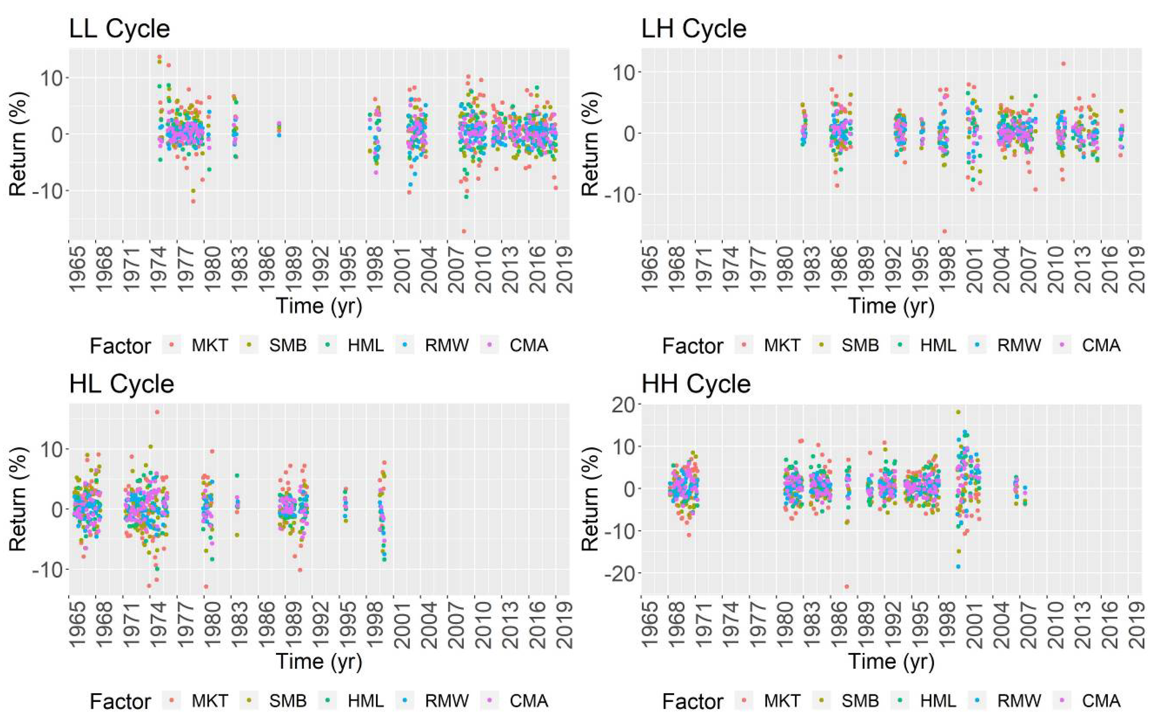
4.2. Results of Interest Rate Cycles and Sentiment Cycles on Five-Factor Returns

Panel A in

Table 3. Interest rate cycles and sentiment cycles on five-factor returns. Panel A presents the significance of five-factor returns in interest rate cycles for Equation (4); Panel B presents the significance of five-factor returns in sentiment cycles for Equation (5). The median of long-term real interest rate is 2.42%, greater than (less than) the median defined as a high-interest rate (low-interest rate) cycle; the median of market sentiment is 0.03, greater than (less than) the median defined as a high-sentiment (low-sentiment) cycle. All t-statistics are based on the Heteroskedasticity-Autocorrelation-Consistent standard errors. **, and *** denote significance at the 5%, and 1% levels, respectively.

Panel A: Interest Rate Cycles					Panel B: Sentiment Cycles
FF5	High-Interest Rate		Low-Interest Rate		FF5	High-Sentiment		Low-Sentiment
	αH	p-Value	αL	p-Value		βH	p-Value	βL	p-Value
MKT	0.0011	0.6653	0.0089	0.0002 ***	MKT	0.0031	0.2142	0.0069	0.0058 ***
SMB	0.0006	0.7339	0.0042	0.0049 ***	SMB	0.0004	0.7977	0.0044	0.0106 **
HML	0.0056	0.0015 ***	0.0007	0.6053	HML	0.0052	0.0018 ***	0.0012	0.4438
RMW	0.0042	0.0040 ***	0.0012	0.2321	RMW	0.0051	0.0003 ***	0.0003	0.7426
CMA	0.0047	0.0003 ***	0.0011	0.2469	CMA	0.0041	0.0007 ***	0.0017	0.105

shows the significance of the five-factor returns in the interest rate cycles. The value, profitability, and investment factors are significant in the high-interest rate cycle but not in the low-interest rate cycle. The market and size factors are significant in the low-interest rate cycle but not in the high-interest rate cycle. As the low-interest rate cycle benefits expansionary monetary policy, the size factor is speculated to obtain a higher premium. Similarly, Jensen and Mercer (2002) found that monetary policy has an obvious asymmetric effect on the size factor for the small-cap premium. Moreover, the value factor has asymmetric risks in the business cycle (Zhang 2005). The significance of the value factor in the high-interest rate cycle can also explain the correlation between the value premium and the rising long-term interest rates (Black et al. 2009).

Panel B in Table 3 shows the significance of five-factor returns in the sentiment cycles. Impressively, the value, profitability, and investment factors are significant in the high-sentiment cycle but not in the low-sentiment cycle. Similarly, the market and size factors are significant only in the low-sentiment cycle. In brief, the size factor is significant in the low-sentiment cycle, and the size premium is accompanied by the effect of return reversal in the high-sentiment cycle. The value factor is only significant in the high-sentiment cycle, in contrast to previous studies in which the value factor does not differ in high- and low-sentiment periods (Baker and Wurgler 2006; Stambaugh et al. 2012). Evidently, the behavioural biases that are driven by investors’ overreactions and underreactions during the high- and low-sentiment cycles cause asymmetric effects on the value factor.

Overall, the interest rate cycles and sentiment cycles asymmetrically affect the five-factor returns, and the factor premium seems to be intimately associated with market cycles. Regarding the macroeconomic and sentiment circumstances in business cycles, the supportive monetary policy that initiates low-interest rate cycles and the investors’ risk aversion during the low-sentiment cycles remarkably affects the market and size factors. We can assume that this effect is connected to the investment cycles accompanying bear markets and recovery periods following economic recessions. Additionally, during high-interest rate and high-sentiment cycles, the bull market and positive sentiment remarkably drive the value, profitability, and investment factors.

4.3. Results of Interest Rate Cycles and Sentiment Cycles on Stock Returns

Panel A in

Table 4. Interest rate cycles and sentiment cycles on stock returns. Panel A presents the five-factor adjusted returns of the S&P 500 in interest rate cycles for Equation (6); Panel B presents the five-factor adjusted returns of the S&P 500 in sentiment cycles for Equation (7). The median of long-term real interest rate is 2.42%, greater than (less than) the median defined as a high-interest rate (low-interest rate) cycle; the median of market sentiment is 0.03, greater than (less than) the median defined as a high-sentiment (low-sentiment) cycle. All t-statistics are based on the Heteroskedasticity-Autocorrelation-Consistent standard errors. *, **, and *** denote significance at the 10%, 5%, and 1% levels, respectively.

Panel A: Interest Rate Cycles				Panel B: Sentiment Cycles
Variables	Coefficient	t-Statistics	p-Value	Variables	Coefficient	t-Statistics	p-Value
DrH	0.0024	8.864	0.0000 ***	DsH	0.0018	6.9912	0.0000 ***
DrL	0.0001	0.4152	0.6781	DsL	0.0008	2.8437	0.0046 ***
MKT	0.9987	194.0783	0.0000 ***	MKT	0.9974	191.0676	0.0000 ***
SMB	−0.1658	−23.3289	0.0000 ***	SMB	−0.1663	−23.1701	0.0000 ***
HML	0.0375	4.002	0.0001 ***	HML	0.0383	3.9306	0.0001 ***
RMW	0.0515	4.2948	0.0000 ***	RMW	0.0518	4.2941	0.0000 ***
CMA	0.0307	1.9104	0.0565 *	CMA	0.0326	1.9933	0.0467 **
Adj. R²	0.9902			Adj. R²	0.9897
Obs. (N)	641			Obs. (N)	641

shows the asymmetric effect of interest rate cycles on S&P 500 returns, which supports Hypothesis 1; that is, in the high-interest rate cycle, long-term real interest rates have a significant effect on stock returns with a positive coefficient (0.0024), whilst the low-interest rate cycle has no significant effect on stock returns (the coefficient approaches zero). As a high-interest rate cycle generally occurs in the period of economic expansion, which is normally accompanied by a higher level of inflation, the effect of interest rates on stock returns is relatively significant. In addition, the interest rate cycle also includes a period of negative real interest rates, for which we explore the effect of negative interest rates on stock returns in Section 5.

Panel B in Table 4 also shows the asymmetric effect of sentiment cycles on S&P 500 returns, which also supports Hypothesis 1; that is, the effects of both high- and low-sentiment cycles on S&P 500 returns are significant, where the effect of a high-sentiment cycle on stock returns (coefficient 0.0018) is greater than that of a low-sentiment cycle (coefficient 0.0008). The asymmetric effect of the sentiment cycle is consistent with this inference, and is possibly explained by behavioural finance—investors are more likely to engage in irrational behaviour when market sentiment is improving (Brown and Cliff 2005; Daniel et al. 1998).

4.4. Results of Five-Factor Adjusted Stock Returns in Market Cycles

Table 5. Five-factor adjusted stock returns in market cycles (real interest rate and market sentiment). The table reports five-factor adjusted returns of the S&P 500 in the four market cycles for Equation (8). The median of long-term real interest rate is 2.42%, greater than (less than) the median defined as a high-interest rate (low-interest rate) cycle; the median of market sentiment is 0.03, greater than (less than) the median defined as a high-sentiment (low-sentiment) cycle. Adjusted R-square: 0.9894 (LL), 0.9943 (LH), 0.9896 (HL), 0.9899 (HH). All t-statistics are based on the Heteroskedasticity-Autocorrelation-Consistent standard errors. *, **, and *** denote significance at the 10%, 5%, and 1% levels, respectively.

Low-Interest Rate, Low-Sentiment (LL)				Low-Interest Rate, High-Sentiment (LH)
	Coefficient	t-Statistics	p-Value		Coefficient	t-Statistics	p-Value
α0	−0.0004	−1.2063	0.2293 *	α0	0.0007	2.5669	0.0114 **
MKT	1.0045	100.7429	0.0000 ***	MKT	1.0103	135.173	0.0000 ***
SMB	−0.1608	−10.8232	0.0000 ***	SMB	−0.1617	−12.3898	0.0000 ***
HML	0.0214	1.4297	0.1545	HML	−0.0043	−0.2074	0.836
RMW	0.0211	0.8392	0.4025	RMW	0.0162	0.9154	0.3617
CMA	0.0378	1.348	0.1793	CMA	0.1082	5.0722	0.0000 ***
High-Interest Rate, Low-Sentiment (HL)				High-Interest Rate, High-Sentiment (HH)
	Coefficient	t-Statistics	p-Value		Coefficient	t-Statistics	p-Value
α0	0.0022	5.4594	0.0000 ***	α0	0.0028	6.5045	0.0000 ***
MKT	0.9908	73.4711	0.0000 ***	MKT	0.9796	72.2565	0.0000 ***
SMB	−0.1467	−11.3989	0.0000 ***	SMB	−0.1826	−12.7264	0.0000 ***
HML	0.0657	3.1738	0.0019 ***	HML	0.0397	1.9107	0.0577 *
RMW	0.1067	4.5282	0.0000 ***	RMW	0.0522	2.7324	0.0069 ***
CMA	0.0286	0.88	0.3805	CMA	−0.0079	−0.2086	0.835

shows the results of the predictive regression model (8). After the five-factor adjusted stock return, the stock market yields the highest monthly excess return (0.28%) in the HH cycle amongst the four market cycles, whilst the lowest and negative monthly excess return (−0.04%) results from the LL cycle. The results in Table 5 support the inference of Hypothesis 2; that is, market cycles have an asymmetric effect on the five-factor adjusted returns of the stock market. This asymmetric effect reflects the monetary easing period with low interest rates; the market capital features a risk appetite that evokes widespread mispricing of the stock market for the convergence of subsequent excess returns. When the interest rates are raised after economic expansion, market sentiment is depressed and the level of investors’ risk aversion increases, resulting in the correction of augmented market valuation for higher excess returns.

In summary, the results in Table 4 and Table 5 show that changes in interest rates and sentiments have an asymmetric effect on the five-factor returns and stock returns, which verifies our Hypotheses 1 and 2. The market factor and size factor are significant in the low-interest rate and low-sentiment cycles. The value factor, profitability factor, and investment factor are significant in the high-interest rate and high-sentiment cycle. Moreover, the five-factor adjusted return of the stock market obtains the highest excess return in the high-interest rate, high-sentiment cycle in contrast to the negative excess return in the low-interest rate, low-sentiment cycle. Consequently, the stock excess returns can be evaluated discriminatively by the market cycles.

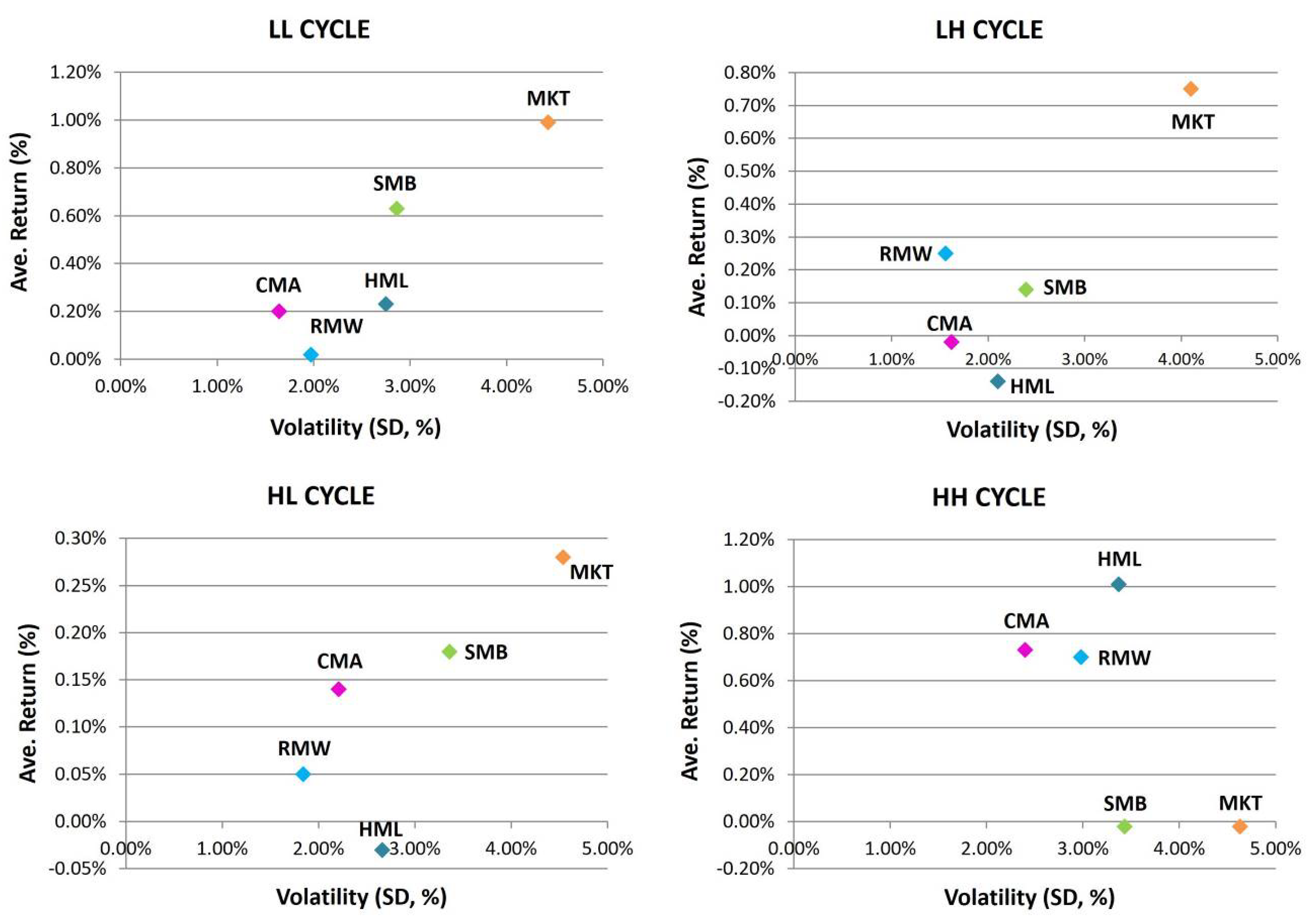
4.5. Factor-Based Investing in Market Cycles

For factor investing strategies, factor premiums should be evaluated in each market cycle as investment horizons in order to optimise portfolio performance.

Table 6. Five-factor returns and Sharpe ratio in market cycles. The sample period spans from July 1965 to December 2018; 642 monthly observations: LL (186), LH (135), HL (139), HH (181). All values and percentages in the table are monthly data (not annualised).

Panel A: Low-Interest Rate, Low-Sentiment (LL)				Panel B: Low-Interest Rate, High-Sentiment (LH)
	Mean	Std Dev	Sharpe ratio		Mean	Std Dev	Sharpe ratio
MKT	0.99%	4.43%	0.1759	MKT	0.75%	4.10%	0.1167
SMB	0.63%	2.86%	0.1461	SMB	0.14%	2.39%	−0.0585
HML	0.23%	2.75%	0.0041	HML	−0.14%	2.10%	−0.1979
RMW	0.02%	1.97%	−0.0969	RMW	0.25%	1.56%	−0.0137
CMA	0.20%	1.64%	−0.0099	CMA	−0.02%	1.62%	−0.1841
Panel C: High-Interest Rate, Low-Sentiment (HL)				Panel D: High-Interest Rate, High-Sentiment (HH)
	Mean	Std Dev	Sharpe ratio		Mean	Std Dev	Sharpe ratio
MKT	0.28%	4.54%	−0.0507	MKT	−0.02%	4.63%	−0.1221
SMB	0.18%	3.36%	−0.099	SMB	−0.02%	3.43%	−0.1658
HML	−0.03%	2.66%	−0.2049	HML	1.01%	3.37%	0.1381
RMW	0.05%	1.84%	−0.252	RMW	0.70%	2.98%	0.0508
CMA	0.14%	2.21%	−0.171	CMA	0.73%	2.40%	0.0782

shows the five-factor monthly average returns, volatility, and Sharpe ratios for the bivariate market cycles. Apart from the high-interest rate and high-sentiment cycle, the market factor acquires the best returns in the other three market cycles. In traditional asset pricing models, the market factor can explain most of the return pattern, whereas mainstream active investing does not focus on the market factor. In contrast, the market premium is measured relative to the risk-free yield rather than the long-short portfolio. Hence, the major concerns of investment strategies remain on the other four factors of the FF5 model. In Table 6, the discrepancy of factor premiums across four market cycles produces several consequences for factor screening.

The LL cycle (Panel A, Table 6). Though all five factors generate positive premia, the market factor has the best average return (0.99%), followed by the size factor (0.63%). As the size factor is significant for the low-interest rate cycles and low-sentiment cycles (see Table 3), it is the preferred factor and has the highest Sharpe ratio besides the market factor. An active monetary policy with low-interest rate cycles is conducive to the size factor, whilst the momentum lifecycle effect may lead to a reward reversal following periods of high sentiment of the size factor.

The LH cycle (Panel B, Table 6). The market factor has the best average return (0.75%) followed by the profitability factor (0.25%). As the profitability factor is significant for high-sentiment cycles (see Table 3), it is the optimal factor besides the market factor. However, the profitability factor performs poorly in low-sentiment cycles (LL, HL), in contrast to its better performance in high-sentiment cycles (LH, HH), which normally occur during a rising business cycle. Benefiting from the capital momentum during low-interest rate cycles, the growth stocks of highly profitable companies are mostly pursued by investors as attractive underlying assets.

The HL cycle (Panel C, Table 6). After the market factor, the size factor is the next best factor in terms of average return due to the significance in the low-sentiment cycles (see Table 3). The five-factor returns in the HL cycle are lower on average than in the other three cycles, indicating that, in the cycle of upward interest rates (economic expansion, rising inflation, or monetary tightening) and downward market sentiment (investors’ risk aversion), the five factors do not reveal a rational risk–reward offset.

The HH cycle (Panel D, Table 6). The value factor obtains the highest return (1.01%) with the highest Sharpe ratio amongst the four cycles. As it is significant in the high-interest rate cycles and high-sentiment cycles (see Table 3), the value factor is the optimal factor. Value investing is highly associated with the macroeconomy. Investors usually invest in value stocks in periods of economic booms resulting from the asymmetric risk of the value factor. Moreover, the investment factor does not obtain a relatively better factor premium in any of the four market cycles. As a result of a high positive correlation (see Table 1) and similar factor characteristics (see Table 2) between the investment and value factor, the investment factor appears to be presumably absorbed by the value factor.

In summary, the results indicate that market cycles play a crucial role in investment strategies, which we call the ‘market cycle effect’ of factor-based investing. Figure A1 in Appendix A provides a scatter diagram of the five-factor returns in the four market cycles based on time-series data. Figure A2 in Appendix B exhibits sequentially the risk–return relationship of the five factors in four market cycles.

5. Discussions

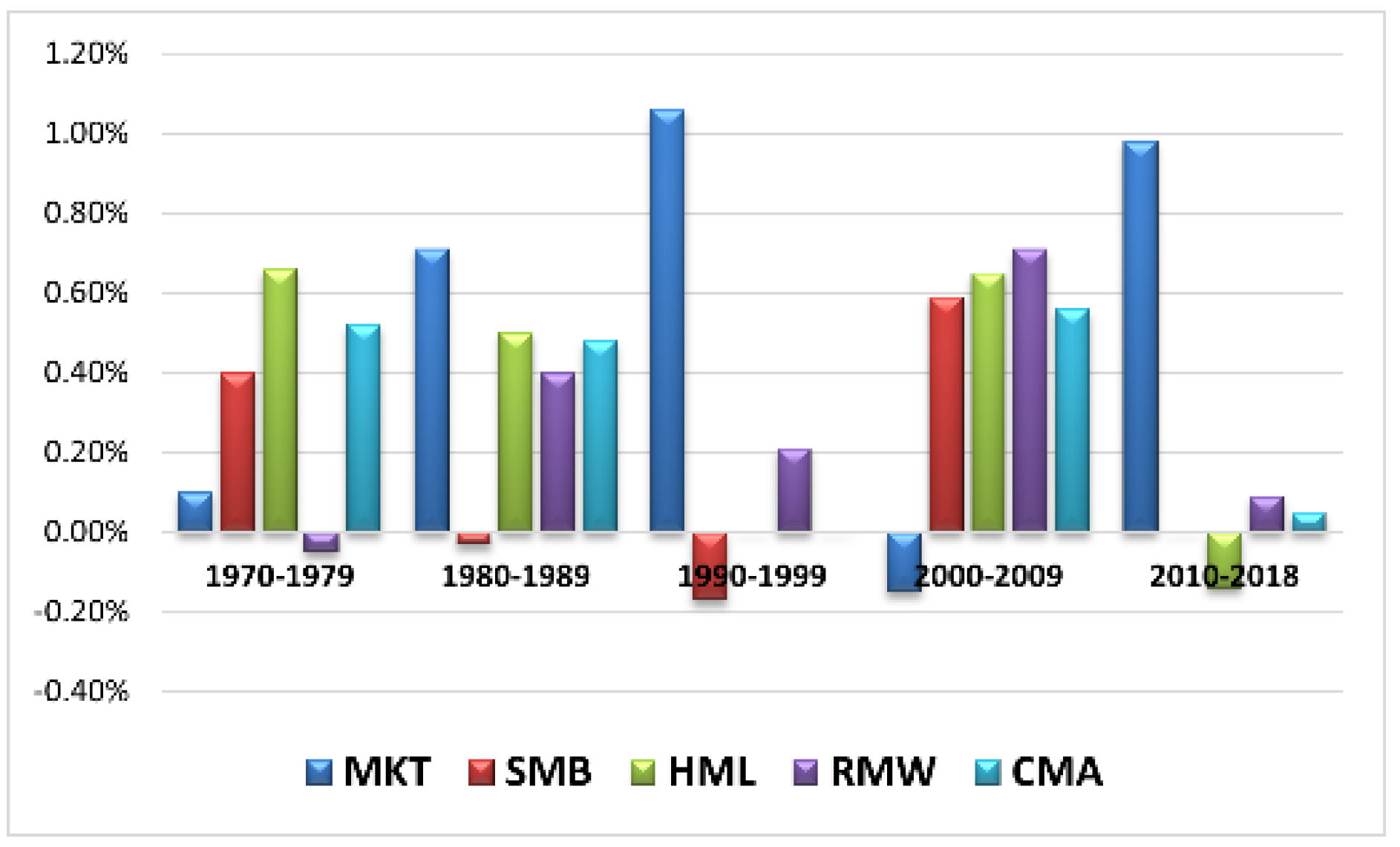
5.1. Five-Factor Returns Based on the Decade

Generally, a universal approach to evaluating factor investing in practice is to survey the factor premium in each decade. Figure 2 shows that, during the period from stagflation in the 1970s to the great inflation in the early 1980s, the Federal Reserve significantly raised its interest rates. The value factor performed best (average monthly return 0.66%) in the high-interest rate and high-sentiment environment. From the late 1980s to the mid-1990s, while bond yields gradually declined, the stock market fell as the post-inflation period set in. Following low-sentiment in the early and late 1990s, the market premium was the highest (average monthly return 1.06%) throughout the decade. After the dot-com bubble burst in 2000, during the low-interest rate and high-sentiment period that began in 2002, the profitability factor attained the highest return (average monthly return 0.71%). The market factor generated a higher-than-average factor premium in the 1990s and 2010s, whilst the size premium and value premium were negative, reflecting the effect of the interest rates and sentiments on the five-factor returns during those decades.

As the Federal Reserve adopted a long-term monetary easing policy in response to the global financial crisis, the market premium has been relatively robust (0.98%). The stock return paradigm during this period showed that the factor premium is almost absorbed by the market factor, with the sum of the other four factors being nearly zero. Figure 3 shows the cumulative returns of the five factors for the entire sample period. The market factor yielded the highest cumulative return (322%), whereas the size factor had the lowest cumulative return (156%). The slope of the cumulative return of the market factor in the post-financial crisis period surged sharply. A possible explanation is that the US financial market experienced negative interest rates numerous times in this business cycle.

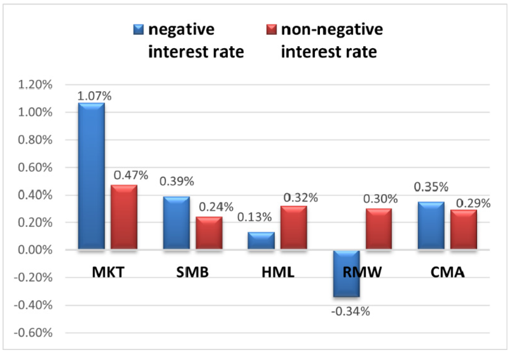
5.2. Five-Factor Returns in Negative Real Interest Rate Cycle

Economic cycles or inflationary environments have caused the US financial market to confront several periods of low-interest rates over the past 50 years, such as in the early 1960s, mid-1970s, mid-to-late 1980s, the early 1990s, the early 2000s, and following the financial crisis in 2008. Periods of negative real interest rates have nevertheless been infrequent. During the sample period, negative interest rates were mainly concentrated after the global financial crisis, from the end of 2008, August 2011 to June 2013, and 2015 to 2016. The US Federal Reserve initiated several interest rate cuts to support its quantitative easing policies. We establish the predictive regression model in order to profile the stock returns through negative real interest rate cycle. Expressed as follows:

RETURN_t = α₀ + β_nDn_t−1 + m_iMKT_t + s_iSMB_t + h_iHML_t + r_iRMW_t + c_iCMA_t + ε_it,

(9)

Table 7. Five-factor adjusted stock returns in negative real interest rate cycle. The table reports five-factor adjusted returns of the S&P 500 in negative real interest rate cycle. The long-term negative real interest rates are extracted and calculated from Shiller Online Data. In Equation (9), if the dummy variable Dn equals 1, indicates negative real interest rate cycle, and 0 otherwise. All t-statistics are based on the Heteroskedasticity-Autocorrelation-Consistent standard errors. **, and *** denote significance at the 5%, and 1% levels, respectively.

Variables	Coefficient	t-Statistics	p-Value
α0	0.0015	7.5624	0.0000 ***
Dn	−0.0041	−8.0967	0.0000 ***
MKT	0.9981	195.3209	0.0000 ***
SMB	−0.1671	−23.5883	0.0000 ***
HML	0.038	4.1087	0.0000 ***
RMW	0.0515	4.2983	0.0000 ***
CMA	0.035	2.1701	0.0304 **
Adj. R²	0.9898

shows the five-factor adjusted returns of the S&P 500 during the period of negative real interest rates. The negative real interest rate cycle creates a higher monthly excess return (0.15%) than during the entire sample period (monthly excess return 0.12% computed by unattached analysis), and the coefficient β_n of the dummy variable Dn is negative (−0.0041), indicating that the negative interest rate cycle has a negative correlation with stock returns. The size factor acquires the only negative coefficient amongst the five factors, consistent with the conclusions of the four market cycles (see Table 5).

Next, we divide the sample data into subsample periods of negative interest rates and non-negative interest rates (including zero interest rates) to distinguish five-factor returns during these two distinct interest rate cycles. The result in Figure 4 shows that, in the negative interest rate cycle, the market factor obtains the highest factor premium, which is more than twice the sum of the average returns of the other four factors. Only the profitability factor has a negative average return. Similarly, the market premium in the negative interest rate cycle is more than twice the market premium in the non-negative interest rate cycle. Correspondingly, the negative value premium during low-interest rates and the negative profitability premium during negative interest rates are possibly caused by the unprecedented cycle of low-interest rate in the US stock market after the global financial crisis.

The historical data of the negative interest rate cycle shows that capital momentum and investor pursuit of higher risk premiums contributed to the soaring market premium. By contrast, growth stocks based on the profitability factor are generally regarded as having a longer equity duration and a high sensitivity to interest rate changes. The negative return of the profitability factor may result from investors’ anxieties about the risk of an economic recession.

In general, the above analyses lead to the empirical results of this study: (1) The value factor gains a better factor premium in the high-interest rate, high-sentiment cycle; and the profitability premium performs better in the low-interest rate, high-sentiment cycle. The above factor performance by decade is fairly consistent with empirical results in this study. Although the size premium approached zero in the low-interest rate cycle in the 2010s, it was probably affected by investor sentiment in preference to large growth stocks during this period. (2) As shown in the empirical results, the value factor and profitability factor are not significant in the low-interest rate cycle. The results in the negative interest rate cycle also indicate that the performance of these two factor premiums is relatively poor. The factor premiums in the negative interest rate cycle are influenced by low-interest rate policy, which is in line with our inferences in market cycles.

6. Robustness

Among the variables used in the empirical analysis, we employ the long-term real interest rate and market sentiment as research variables. Inversely, we employ the opposite variables as robustness tests: the long-term nominal interest rate (US 10-year treasury yield) and direct sentiment indices (University of Michigan Consumer Sentiment Index). The data source for these two variables is derived from the US Federal Reserve.7 As the sample period for consumer sentiment is relatively short (only quarterly data before 1978), our sample period for the robustness analysis is from January 1978 to December 2018, which yielded 492 monthly samples (491 monthly observations in predictive regression). We investigate the effect of interest rates and sentiments on stock returns using the predictive regression models as follows, respectively.

RETURN_t = α_HDrH_t−1 + α_LDrL_t−1 + m_iMKT_t + s_iSMB_t + h_iHML_t + r_iRMW_t + c_iCMA_t + e_it,

(10)

RETURN_t = β_HDsH_t−1 + β_LDsL_t−1 + m_iMKT_t + s_iSMB_t + h_iHML_t + r_iRMW_t + c_iCMA_t + e_it,

(11)

The empirical results in Panels A and B in

Table 8. Nominal interest rate cycles and consumer sentiment cycles on stock returns. Panel A presents the five-factor adjusted returns of the S&P 500 in interest rate cycles, Panel B presents the five-factor adjusted returns of the S&P 500 in sentiment cycles. The median of the long-term nominal interest rate is 5.81%, greater than (less than) the median defined as a high-interest rate (low-interest rate) cycle. The median of consumer sentiment is 89.6, greater than (less than) the median defined as a high-sentiment (low-sentiment) cycle. If dummy variable DrH equals 1, it indicates a high-interest rate cycle, and 0 otherwise; if DrL equals 1, it indicates a low-interest rate cycle, and 0 otherwise. If dummy variable DsH equals 1, it indicates a high-sentiment cycle, and 0 otherwise; if DsL equals 1, it indicates a low-sentiment cycle, and 0 otherwise. All t-statistics are based on the Heteroskedasticity-Autocorrelation-Consistent standard errors. **, and *** denote significance at the 5%, and 1% levels, respectively.

Panel A: Nominal Interest Rate Cycles				Panel B: Consumer Sentiment Cycles
Variables	Coefficient	t-Statistics	p-Value	Variables	Coefficient	t-Statistics	p-Value
DrH	0.0026	8.5855	0.0000 ***	DsH	0.0016	5.0312	0.0000 ***
DrL	−0.0003	−1.1637	0.2451	DsL	0.0006	2.081	0.0380 **
MKT	0.9997	168.7748	0.0000 ***	MKT	1.0016	159.0878	0.0000 ***
SMB	−0.1801	−20.7159	0.0000 ***	SMB	−0.1798	−20.1159	0.0000 ***
HML	0.0267	2.6221	0.0090 ***	HML	0.0281	2.5414	0.0114 **
RMW	0.0502	3.6999	0.0002 ***	RMW	0.0489	3.6333	0.0003 ***
CMA	0.0455	2.3713	0.0181 **	CMA	0.0475	2.4752	0.0137 **
Adj. R²	0.9904			Adj. R²	0.9894
Obs. (N)	491			Obs. (N)	491

show that interest rate cycles and sentiment cycles have an asymmetric effect on S&P 500 returns, which supports Hypothesis 1 and is consistent with the results in Table 4. In Panel A, the long-term nominal interest rate has a significant effect on stock returns with a positive coefficient (0.0026) in the high-interest rate cycle, but has no significant effect on stock returns in the low-interest rate cycle. In Panel B, both high- and low-sentiment cycles are significant for stock returns, whilst the high-sentiment cycle has a greater effect on stock returns (coefficient 0.0016) than the low-sentiment cycle (coefficient 0.0006).

To infer Hypothesis 2, we further verify the asymmetric effect of the four market cycles constituted by two alternative variables on stock returns. The predictive regression model is as follows:

RETURN_t = α₀ + γ_rDr_t−1 + γ_sDs_t−1+ m_iMKT_t + s_iSMB_t + h_iHML_t + r_iRMW_t + c_iCMA_t + e_it,

(12)

According to the results summarised in

Table 9. Five-factor adjusted stock returns in market cycles (nominal interest rate and consumer sentiment). The table reports the five-factor adjusted returns of the S&P 500 in the four market cycles. The median of the long-term nominal interest rate is 5.81%, greater than (less than) the median defined as a high-interest rate (low-interest rate) cycle. The median of consumer sentiment is 89.6, greater than (less than) the median defined as a high-sentiment (low-sentiment) cycle. If the dummy variable Dr equals 1, it indicates a high-interest rate cycle, and 0 otherwise; if the dummy variable Ds equals 1, it indicates a high-sentiment cycle, and 0 otherwise. Adjusted R-square: 0.9962 (LL); 0.9825 (LH); 0.9899 (HL); 0.9921 (HH). All t-statistics are based on the Heteroskedasticity-Autocorrelation-Consistent standard errors. *, **, and *** denote significance at the 10%, 5%, and 1% levels, respectively.

Low-Interest Rate, Low-Sentiment (LL)				Low-Interest Rate, High-Sentiment (LH)
	Coefficient	t-Statistics	p-Value		Coefficient	t-Statistics	p-Value
α0	−0.001	−4.0213	0.0001 ***	α0	0.0005	1.1502	0.2527
MKT	1.0079	160.7171	0.0000 ***	MKT	0.9847	46.8232	0.0000 ***
SMB	−0.1554	−12.0788	0.0000 ***	SMB	−0.1239	−6.7069	0.0000 ***
HML	0.015	1.0614	0.2905	HML	0.0253	0.8877	0.3767
RMW	0.0243	1.7982	0.0745 *	RMW	0.0416	1.0272	0.3067
CMA	0.0293	1.5436	0.1252	CMA	0.0202	0.5362	0.593
High-Interest Rate, Low-Sentiment (HL)				High-Interest Rate, High-Sentiment (HH)
	Coefficient	t-Statistics	p-Value		Coefficient	t-Statistics	p-Value
α0	0.0028	5.3776	0.0000 ***	α0	0.0024	5.6847	0.0000 ***
MKT	0.9842	72.9481	0.0000 ***	MKT	0.9991	59.0599	0.0000 ***
SMB	−0.2137	−12.6005	0.0000 ***	SMB	−0.1918	−7.2861	0.0000 ***
HML	−0.026	−0.9459	0.3463	HML	−0.0084	−0.3709	0.7113
RMW	0.0515	1.6182	0.1086	RMW	0.0911	3.2039	0.0017 ***
CMA	0.1031	2.5057	0.0137 **	CMA	0.0912	2.6977	0.0079 ***

, after the five-factor adjustment, the stock market has the lowest and negative monthly excess return (−0.1%) in the low-interest rate and low-sentiment cycle, which contrasts with the relatively higher and positive monthly excess returns (0.24%) in the high-interest rate and high-sentiment cycle. This result is identical to the conclusion in Table 5 and supports Hypothesis 2. Even though the highest monthly excess return (0.28%) arises in the high-interest rate and low-sentiment cycle, which is distinct from the high-interest rate and high-sentiment cycle in Table 5, it still does not negate Hypothesis 2.

The above findings illustrate the asymmetric effects of interest rates, sentiments, and market cycles on stock returns. Intuitively, Figure 5 shows that the real interest rate and nominal interest rate have roughly equivalent tendencies. The difference between the two lies in the inflation rate, where the real interest rate is the implicit information of the negative real interest rates. Figure 6 shows that, after the global financial crisis, market sentiment deviated significantly from consumer sentiment. Although the global environment of low-interest rates during this period supported bullish consumer confidence, in the financial market, the market sentiment tended to be depressed, showing sluggish oscillation.

7. Conclusions

In this article, we employ market cycles based on Shiller’s market interest rate and Baker–Wurgler’s market sentiment with the FF5 model to verify three return patterns of the asset pricing model: (1) Market risk premium: from the perspective of market cycles, the market factor has a comparatively reliable risk premium in three cycles, except the high-interest rate and high-sentiment cycle. Even taking the decade as the base period, the market premium shows superior returns in the 1990s and 2010s. ‘Beating the market’ in the low-interest rate (or negative interest rate) cycle of loose funds has become increasingly difficult. (2) Factor premium: The empirical analysis of five-factor returns in the US stock market reveals that the five factors dominate separately in different market cycles. Essentially, the factor premium appears to be the risk compensation for the five factors in market cycles. Presumably, the disappearance of the value premium in the 1990s and 2010s seems to highlight the role of market cycles in the five-factor returns. (3) Excess return: Our findings show that the high-interest rate and high-sentiment cycle generates a higher excess return, whilst the low-interest rate and low-sentiment cycle produces a lower excess return. Even if the alternative variables of interest rates and sentiments are substituted in the robustness analysis, our hypotheses are still convincing.

In terms of factor investing strategies, in a broad multi-factor portfolio, the value investing strategy of the value factor performs best in the high-interest rate and high-sentiment cycle. The growth investing strategy based on the profitability factor outperforms in the high-sentiment cycles. The long-short portfolio with the size factor obtains better returns in the low-interest rate and low-sentiment cycle. Additionally, our evidence reveals that the value factor is significant in the high-sentiment cycle and insignificant in the low-sentiment cycle, which differs from the previous studies.

Considering the factor characteristics of the FF5 model, the results of the asymmetric GARCH model present an asymmetric effect on volatility; that is, the market, size, and profitability factors exhibit similar factor characteristics for changes in market interest rate, whilst the value and investment factors exhibit similar factor characteristics for changes in market sentiment. Furthermore, the size factor has an asymmetric leverage effect on the changes in interest rates and sentiments, and the profitability factor is the only one amongst the five factors that does not possess a risk premium for the changes in interest rates or sentiments. Importantly, understanding the internal mechanism of interest rate and sentiment variables on the asymmetry of five-factor characteristics requires more empirical evidence based on econometrics.

This study demonstrates the asymmetric effect on stock returns and five-factor returns through market cycles. In contrast to the previous factor spanning test, we provide a cyclical template for investment theory—factor-based investing in market cycles. We further assume that the market cycle has an asymmetric effect on cross-asset classes and cross markets, where, of course, there may be limitations to the lack of market sentiment indices besides the US financial market. The specific formation of factor-based investing involves investment targets (factors), funds (interest rate policies), and investor behaviours (sentiments). Therefore, future research can be extended to integrate an asset pricing model that incorporates the interest rate and sentiment variables. Regardless of whether factor premia are derived from the interpretation of risk or behaviour premia, investors should identify where we are in the cycle. By penetrating market cycles as investment horizons, investors are able to position investment strategies to optimise portfolio performance.

References

1. Abdullah, Dewan A., and Steven C. Hayworth. 1993. Macroeconometrics of Stock Price Fluctuations. Quarterly Journal of Business and Economics 32: 50–67. [Google Scholar]
2. Amenc, Noël, Mikheil Esakia, Felix Goltz, and Ben Luyten. 2019. Macroeconomic Risks in Equity Factor Investing. The Journal of Portfolio Management 45: 39–60. [Google Scholar] [CrossRef]
3. Ang, Andrew, Ked Hogan, and Sara Shores. 2018. Factor Risk Premiums and Invested Capital: Calculations with Stochastic Discount Factors. Journal of Asset Management 19: 145–55. [Google Scholar] [CrossRef]
4. Arnott, Robert D., Campbell R. Harvey, Vitali Kalesnik, and Juhani T. Linnainmaa. 2021. Reports of Value’s Death May Be Greatly Exaggerated. Financial Analysts Journal 77: 44–67. [Google Scholar] [CrossRef]
5. Arnott, Robert D., Jason Hsu, and Philip Moore. 2005. Fundamental Indexation. Financial Analysts Journal 61: 83–99. [Google Scholar] [CrossRef]
6. Asness, Clifford, Andrea Frazzini, Ronen Israel, and Tobias Moskowitz. 2015. Fact, Fiction, and Value Investing. The Journal of Portfolio Management 42: 34–52. [Google Scholar] [CrossRef]
7. Asness, Clifford S., Jacques A. Friedman, Robert J. Krail, and John M. Liew. 2000. Style Timing. The Journal of Portfolio Management 26: 50–60. [Google Scholar] [CrossRef]
8. Asness, Clifford S., Tobias J. Moskowitz, and Lasse Heje Pedersen. 2013. Value and Momentum Everywhere. The Journal of Finance 68: 929–85. [Google Scholar] [CrossRef] [Green Version]
9. Baker, Malcolm, and Jeffrey Wurgler. 2006. Investor Sentiment and the Cross-Section of Stock Returns. The Journal of Finance 61: 1645–80. [Google Scholar] [CrossRef] [Green Version]
10. Baker, Malcolm, and Jeremy C Stein. 2004. Market Liquidity as a Sentiment Indicator. Journal of Financial Markets 7: 271–99. [Google Scholar] [CrossRef] [Green Version]
11. Baks, Klaas, and Charles Frederick Kramer. 1999. Global Liquidity and Asset Prices: Measurement, Implications, and Spillovers. IMF working paper. SSRN Electronic Journal 99: 168. [Google Scholar] [CrossRef]
12. Banz, Rolf W. 1981. The Relationship between Return and Market Value of Common Stocks. Journal of Financial Economics 9: 3–18. [Google Scholar] [CrossRef] [Green Version]
13. Barberis, Nicholas, and Andrei Shleifer. 2003. Style Investing. Journal of Financial Economics 68: 161–99. [Google Scholar] [CrossRef] [Green Version]
14. Barberis, Nicholas, and Ming Huang. 2008. Stocks as Lotteries: The Implications of Probability Weighting for Security Prices. American Economic Review 98: 2066–100. [Google Scholar] [CrossRef] [Green Version]
15. Black, Angela J., Bin Mao, and David G. McMillan. 2009. The Value Premium and Economic Activity: Long-Run Evidence from the United States. Journal of Asset Management 10: 305–17. [Google Scholar] [CrossRef]
16. Blitz, David, Eric Falkenstein, and Pim van Vliet. 2014. Explanations for the Volatility Effect: An Overview Based on the CAPM Assumptions. The Journal of Portfolio Management 4: 61–76. [Google Scholar] [CrossRef]
17. Blitz, David. 2015. Factor Investing Revisited. The Journal of Index Investing 6: 7–17. [Google Scholar] [CrossRef]
18. Blitz, David. 2020. Factor Performance 2010–2019: A Lost Decade? The Journal of Index Investing 11: 57–65. [Google Scholar] [CrossRef]
19. Bollerslev, Tim, Ray Y. Chou, and Kenneth F. Kroner. 1992. Arch Modeling in Finance. Journal of Econometrics 52: 5–59. [Google Scholar] [CrossRef]
20. Brown, Gregory W., and Michael T. Cliff. 2004. Investor Sentiment and the near-Term Stock Market. Journal of Empirical Finance 11: 1–27. [Google Scholar] [CrossRef]
21. Brown, Gregory W., and Michael T. Cliff. 2005. Investor Sentiment and Asset Valuation. The Journal of Business 7: 405–40. [Google Scholar] [CrossRef]
22. Campbell, John Y. 1987. Stock Returns and the Term Structure. Journal of Financial Economics 18: 373–99. [Google Scholar] [CrossRef] [Green Version]
23. Campbell, John Y., and Robert J. Shiller. 1988. Stock Prices, Earnings, and Expected Dividends. The Journal of Finance 43: 661–76. [Google Scholar] [CrossRef]
24. Campbell, John Y., and Robert J. Shiller. 1998. Valuation Ratios and the Long-Run Stock Market Outlook. The Journal of Portfolio Management 24: 11–26. [Google Scholar] [CrossRef]
25. Carhart, Mark M. 1997. On Persistence in Mutual Fund Performance. The Journal of Finance 52: 57–82. [Google Scholar] [CrossRef]
26. Daniel, Kent, and Sheridan Titman. 1998. Characteristics or Covariances? The Journal of Portfolio Management 24: 24–33. [Google Scholar] [CrossRef]
27. Daniel, Kent, David Hirshleifer, and Avanidhar Subrahmanyam. 1998. Investor Psychology and Security Market under- and Overreactions. The Journal of Finance 53: 1839–85. [Google Scholar] [CrossRef] [Green Version]
28. De Bondt, Werner F., and Richard Thaler. 1985. Does the Stock Market Overreact? The Journal of Finance 40: 793–805. [Google Scholar] [CrossRef]
29. Dimson, Elroy, Paul Marsh, and Mike Staunton. 2017. Factor-Based Investing: The Long-Term Evidence. The Journal of Portfolio Management 43: 15–37. [Google Scholar] [CrossRef]
30. Engle, Robert F., David M. Lilien, and Russell P. Robins. 1987. Estimating Time Varying Risk Premia in the Term Structure: The ARCH-M Model. Econometrica 55: 391. [Google Scholar] [CrossRef]
31. Fama, Eugene F., and Kenneth R. French. 1993. Common risk factors in the returns on stocks and bonds. Journal of Financial Economics 33: 3–56. [Google Scholar] [CrossRef]
32. Fama, Eugene F., and Kenneth R. French. 2006. Profitability, Investment and Average Returns. Journal of Financial Economics 82: 491–518. [Google Scholar] [CrossRef]
33. Fama, Eugene F., and Kenneth R. French. 2015. A Five-Factor Asset Pricing Model. Journal of Financial Economics 116: 1–22. [Google Scholar] [CrossRef] [Green Version]
34. Fama, Eugene F., and Kenneth R. French. 2017. International Tests of a Five-Factor Asset Pricing Model. Journal of Financial Economics 123: 441–63. [Google Scholar] [CrossRef]
35. Fama, Eugene F., and Kenneth R. French. 2021. The Value Premium. The Review of Asset Pricing Studies 11: 105–21. [Google Scholar] [CrossRef]
36. Flannery, Mark J., and Christopher M. James. 1984. The Effect of Interest Rate Changes on the Common Stock Returns of Financial Institutions. The Journal of Finance 39: 1141–53. [Google Scholar] [CrossRef]
37. Glosten, Lawrence R., Ravi Jagannathan, and David E. Runkle. 1993. On the Relation between the Expected Value and the Volatility of the Nominal Excess Return on Stocks. The Journal of Finance 48: 1779–1801. [Google Scholar] [CrossRef]
38. Gompers, Paul A., and Andrew Metrick. 2001. Institutional Investors and Equity Prices. The Quarterly Journal of Economics 116: 229–59. [Google Scholar] [CrossRef]
39. Gregoriou, Andros, Jerome V. Healy, and Huong Le. 2019. Prospect Theory and Stock Returns: A Seven Factor Pricing Model. Journal of Business Research 101: 315–22. [Google Scholar] [CrossRef]
40. Harvey, Campbell R., Yan Liu, and Heqing Zhu. 2015. … And the Cross-Section of Expected Returns. Review of Financial Studies 29: 5–68. [Google Scholar] [CrossRef] [Green Version]
41. Hirshleifer, David. 2001. Investor Psychology and Asset Pricing. The Journal of Finance 56: 1533–97. [Google Scholar] [CrossRef]
42. Horowitz, Joel L., Tim Loughran, and N. E. Savin. 2000. Three Analyses of the Firm Size Premium. Journal of Empirical Finance 7: 143–53. [Google Scholar] [CrossRef]
43. Israel, Ronen, Kristoffer Laursen, and Scott Richardson. 2021. Is (Systematic) Value Investing Dead? The Journal of Portfolio Management 47: 38–62. [Google Scholar] [CrossRef]
44. Jegadeesh, Narasimhan, and Sheridan Titman. 1993. Returns to Buying Winners and Selling Losers: Implications for Stock Market Efficiency. The Journal of Finance 48: 65–91. [Google Scholar] [CrossRef]
45. Jensen, Gerald R., and Jeffrey M. Mercer. 2002. Monetary Policy and the Cross-Section of Expected Stock Returns. Journal of Financial Research 25: 125–39. [Google Scholar] [CrossRef]
46. Jensen, Gerald R., and Robert R. Johnson. 1995. Discount Rate Changes and Security Returns in the U.S., 1962–1991. Journal of Banking & Finance 19: 79–95. [Google Scholar]
47. Lakonishok, Josef, Andrei Shleifer, and Robert W. Vishny. 1994. Contrarian Investment, Extrapolation, and Risk. The Journal of Finance 49: 1541–78. [Google Scholar] [CrossRef]
48. Lee, Charles M. C., and Bhaskaran Swaminathan. 2000. Price Momentum and Trading Volume. The Journal of Finance 55: 2017–69. [Google Scholar] [CrossRef]
49. Liu, Ryan. 2015. Profitability Premium: Risk or Mispricing. Working Paper. Berkeley: University of California at Berkeley. [Google Scholar]
50. Lucas, André, Ronald van Dijk, and Teun Kloek. 2002. Stock Selection, Style Rotation, and Risk. Journal of Empirical Finance 9: 1–34. [Google Scholar] [CrossRef] [Green Version]
51. Novy-Marx, Robert. 2013. The Other Side of Value: The Gross Profitability Premium. Journal of Financial Economics 108: 1–28. [Google Scholar] [CrossRef] [Green Version]
52. Novy-Marx, Robert, and Mihail Velikov. 2016. A Taxonomy of Anomalies and Their Trading Costs. Review of Financial Studies 29: 104–47. [Google Scholar] [CrossRef]
53. Peng, Yulei, and Anastasia Zervou. 2022. Monetary Policy Rules and the Equity Premium in a Segmented Markets Model. Journal of Macroeconomics 73: 103448. [Google Scholar] [CrossRef]
54. Rupande, Lorraine, Hilary Tinotenda Muguto, and Paul-Francois Muzindutsi. 2019. Investor Sentiment and Stock Return Volatility: Evidence from the Johannesburg Stock Exchange. Cogent Economics & Finance 7: 1600233. [Google Scholar]
55. Ryan, Nina, Xinfeng Ruan, Jin E. Zhang, and Jing A. Zhang. 2021. Choosing Factors for the Vietnamese Stock Market. Journal of Risk and Financial Management 14: 96. [Google Scholar] [CrossRef]
56. Schmeling, Maik. 2009. Investor Sentiment and Stock Returns: Some International Evidence. Journal of Empirical Finance 16: 394–408. [Google Scholar] [CrossRef] [Green Version]
57. Shiller, Robert J., Laurence Black, and Farouk Jivraj. 2020. Cape and the COVID-19 Pandemic Effect. SSRN Electronic Journal. [Google Scholar] [CrossRef]
58. Stambaugh, Robert F., Jianfeng Yu, and Yu Yuan. 2012. The Short of It: Investor Sentiment and Anomalies. Journal of Financial Economics 104: 288–302. [Google Scholar] [CrossRef] [Green Version]
59. Yogo, Motohiro. 2006. A Consumption-Based Explanation of Expected Stock Returns. The Journal of Finance 61: 539–80. [Google Scholar] [CrossRef] [Green Version]
60. Zhang, Lu. 2005. The Value Premium. The Journal of Finance 60: 67–103. [Google Scholar] [CrossRef]
Figure 1. Five-factor returns and conditional variances of the GJR-GARCH(1,1)-M model. The left-hand side shows the effect of interest rates on five-factor asymmetric GARCH model, the right-hand side shows the effect of sentiments on five-factor asymmetric GARCH model. Blue lines and red lines indicate the factor return and conditional covariance, respectively. MKT, SMB, HML, RMW, and CMA denote the monthly return of the market, size, value, profitability, and investment factors, respectively. The sample period spans from July 1965 to December 2018.
Jrfm 15 00460 g001
Figure 2. Five-factor premiums by decade (1970–2018).
Jrfm 15 00460 g002
Figure 3. Cumulative returns of the five factors (1965–2018).
Jrfm 15 00460 g003
Figure 4. Average five-factor returns in periods of negative and non-negative interest rates.
Jrfm 15 00460 g004
Figure 5. Changes in long-term real and nominal interest rates (1978–2018).
Jrfm 15 00460 g005
Figure 6. Changes in market sentiment and consumer sentiment (1978–2018).
Jrfm 15 00460 g006