Do ESG Ratings Reduce the Asymmetry Behavior in Volatility?

Abstract

It is well noted in the literature that volatility responds differently to positive and negative shocks. In this paper, we explore the impact of ESG ratings on such asymmetric behavior of volatility. For this analysis, we use the return data, ESG ratings, and solvency ratios of the constituent stocks of S&P Europe 350 for the period January 2016–December 2021. We apply autoregressive moving average models for the conditional means and GARCH and stochastic volatility models for the conditional variances to estimate the asymmetry coefficients. Afterwards, these coefficients are regressed via Arellano–Bond and lagged first difference methods to estimate the impact of ESG ratings. Our findings confirm that stocks of riskier firms are more likely to suffer from asymmetry behavior of volatility. We also confirm that firm leverage is linked to this asymmetry behavior. We found evidence that the impact of ESG ratings was negative before COVID-19, but positive afterwards. For some sectors, higher ESG ratings are linked to higher asymmetry. Finally, we found that during COVID-19, the asymmetry behavior became more pronounced.

1. Introduction

One of the stylized facts about financial returns is the leverage effect, which refers to the negative correlation between the current return shocks and future volatility shocks. A special case of the leverage effect is the asymmetric effects in volatility, which implies that a negative return shock would increase the volatility much more than a positive return shock of the same magnitude. It may even be the case that positive return shocks would decrease future volatility. Hence, as explained in Asai et al. (2006), not all asymmetric effects would imply leverage effects.

There have been many papers proposed to capture asymmetric effects in the conditional volatility models such as the Glosten, Jagganathan, and Runkle (GJR)-GARCH of Glosten et al. (1993), the asymmetric GARCH (AGARCH) and nonlinear asymmetric GARCH (NAGARCH) of Engle and Ng (1993), and the exponential GARCH (EGARCH) of Nelson (1991), among many others. Teräsvirta (2009) gives a good overview of the conditional volatility models, including those that adapt for asymmetric effects.

The asymmetry behavior in volatility is in a way related to how the investors react to good and bad news (Black 1976; Christie 1982; Nelson 1991 among others). Bad news brings about more uncertainty, hence increased risk, in the stocks they invest in. Christie (1982) points out that the asymmetric effect can be related to the financial leverage of the firms. As noted in Ghysels et al. (1996), falling stock prices imply a lower equity value for the firms, and if the debt level stays the same, this implies an increased leverage for the firms. This, in turn, would bring more uncertainty, and hence more volatility. However, Black (1976), Christie (1982), Schwert (1989), and Ghysels et al. (1996) note that financial leverage of firms may not be sufficient to explain the leverage effects in financial returns.

There are some contradictory findings in the literature with regard to explaining leverage effects with firm leverage. Choi and Richardson (2016) for example find evidence that financial leverage has a significant and large influence on the equity volatility. However, Hens and Steude (2009) state that the leverage effect does not necessarily come from the financial leverage of the firms.

In this paper, we explore if firms maintain higher ESG profiles, the asymmetric effects in the volatility of their stocks is reduced. In other words, we analyze if high ESG ratings would reduce the size of the increase in the volatility of a stock in the face of negative news. The motivation follows from the fact that investors may perceive stocks with higher ESG profiles as long-run investments and hence less risky. Therefore, their reaction to bad news is relatively more stable. The argument here is in line with the discussion of Cerqueti et al. (2021) that ESG-related assets are not likely to be sold in the event of crisis since the investors consider them as long-term investments. Moreover, they are not yet commonly preferred assets; hence, they are less vulnerable to shocks. On the other hand, it has been documented that the investors may see ESG-related activities as an additional risk (see, for example, Lundgren et al. 2018; Ionescu et al. 2019; Friede et al. 2015). Although the impact of ESG ratings on the financial performances of firms is studied extensively in the literature, to the best of our knowledge, there is no work relating it to the asymmetry behavior in volatility.

The chosen research problem is important at least in two directions. Stock market investors definitely care about all the possible leading information that could signal how the stock returns and volatility will evolve. If a firm’s stock is suffering from asymmetric effects, it is valuable to investors to know what further ESG-related investments would bring about. Naturally, the investors would consider if the firm is taking additional risks or perhaps taking a step to reduce the asymmetric effect. On the other hand, asymmetric effects that individual stocks are suffering can be related to the overall risk of the stock market. Firms who are riskier than the market, suffering from the asymmetric effect, and taking additional risks while engaging in ESG-related activities bring about higher threat to the stock market. Hence, researchers and practitioners working in the field of systemic risk would find the research of this paper useful.

For this analysis, we used the constituent stocks of S&P Europe 350 for the period January 2016–December 2021. The data partly correspond to the COVID-19 pandemic period, which provides an option to study its influence on the partial effects. We take the return data of each year separately and fit autoregressive moving average models to each stock return, taking into account the outliers and market returns. Afterwards, we fit the GJR-GARCH model of Glosten et al. (1993), the AGARCH and NAGARCH models of Engle and Ng (1993), and the SVL model of Harvey and Shephard (1996) to each series. Therefore, for each year between 2016 and 2021 and for each stock, we obtain asymmetric effects and leverage effects’ coefficients. Using the ESG ratings we collected for each stock and the solvency ratios of each corresponding firm, we estimate fixed effects models to study the effect of ESG ratings on the asymmetry coefficients. To alleviate the heteroscedasticity of using an estimated dependent variable, we weight the regressors by the standard error of the dependent variable following Hornstein and Greene (2012). On the other hand, we apply Arellano–Bond and lagged first difference methods to account for possible reverse causality (see Arellano and Bond 1991; Allison 2009; Leszczensky and Wolbring 2022).

Our findings suggest that for stock prices, firms that are riskier than the market, i.e., firms with higher betas, are more likely to suffer from the asymmetric behavior. One explanation could be that if the market is experiencing a shock and a stock is riskier than the market, the investors are likely to react strongly, and this reflects as a strong jump in the volatility process. We also found that solvency ratios are negatively linked with the asymmetry behavior. Since the solvency ratio is related to the inverse of firm leverage, we can confirm the existing results in the literature that firm leverage is linked to the asymmetry behavior. We also found that during COVID-19, the asymmetry behavior in volatility was higher on average. This can be explained by the increased uncertainty during the COVID-19 time, as it is understandable that investors could react more drastically to negative shocks under uncertainty. In terms of the impact of ESG ratings, the results were hard to generalize, as the effects were sector-specific. The results suggested that high ESG ratings are associated with lower asymmetry before COVID-19, but with higher asymmetry after COVID-19. We also found that higher ESG ratings are associated with higher asymmetry for the Communications, Financials, Healthcare, Industrials, and Utilities sectors. We could extrapolate this finding to the Consumer Discretionary, Energy, and Real Estate sectors as well.

The rest of the paper is structured as follows. Section 2 gives a literature review on the asymmetric effects and leverage effects and also on the studies of the impact of ESG ratings on the financial performances of firms. Section 3 explains the conditional mean and conditional variance models used to extract the asymmetry coefficients and afterwards describes the fixed effects methods used for exploring the causality between ESG ratings and asymmetry behavior. Section 4 describes the returns data of the stocks and also provides descriptive statistics and histograms on the annual betas, ESG ratings, and solvency ratios of the firms by country and sector. Section 5 discusses the findings on the asymmetry coefficients and on the impact of ESG ratings following the Arellano–Bond estimation method. Section 6 discusses the other methods considered for robustness. In particular, we present here the results of the lagged first difference method and compare the findings. Section 7 concludes and gives suggestions for further research.

2. Literature Review

2.1. Asymmetric Effect and Leverage Effect in Volatility

One of the stylized facts about financial returns is the negative correlation between current returns and future volatility (Ghysels et al. 1996). This observation was noted by many papers such as Black (1976); Christie (1982); and Nelson (1991) and was considered conventionally under the general name of “leverage effects”.

The financial econometrics literature mainly mentions two possible sources for the leverage effects, namely the firm leverage and volatility feedback effects (Carr and Wu 2017). There have been many papers discussing that the leverage effect is due to the financial leverage positions of the firms. The general idea behind this way of thought is that falling stock prices imply a lower equity value for the firms, and given the same level of debt, it implies an increased leverage for the firms. This reflects as future uncertainty, hence as higher future volatility (Christie 1982; Choi and Richardson 2016). In our paper, we use asset-based solvency ratios of the firms as a proxy for the inverse of the financial leverage of the firms (Wagner 2003). The solvency ratio represent a firm’s ability to cover the long-term debt.

While this could indeed be one reason behind the leverage effect, some authors defended that there is more to it than just the financial leverage. Black (1976), Christie (1982), Schwert (1989), Ghysels et al. (1996), and Hens and Steude (2009), among others, suggest that financial leverage alone cannot explain the leverage effects in volatility.

One other explanation for the leverage effects is the volatility feedback. A particular firm’s risk position can change over time with respect to the market, and given the expectations on the cash flow, the increased future risk reflects in the current stock price of the firm, often reducing it (Carr and Wu 2017; Bekaert and Wu 2000; Campbell and Hentschel 1992). Indeed, this is also mentioned in Adrian and Shin (2010), that firms may change their financial leverage positions according to the market conditions. On the other hand, Cho and Engle (1999) suggests that the leverage effect could result from financial leverage, as well as the market risk premium. The take-away point from the volatility feedback concept for our paper is that higher risk compared to the market is one source that feeds the leverage effect. This justifies our choice of using betas of firms as one of the regressors.

Asymmetric effects in volatility comprise a particular case of the leverage effects. Often, these two terms are confused with each other. Asai et al. (2006) and Asai and McAleer (2011) clearly explain different types of asymmetry and how they relate to leverage effects. In asymmetric effects, the impact of positive and negative shocks on the future volatility can be different. In particular, a negative shock increases future volatility more than a positive shock of the same magnitude would. It is also possible that a positive shock could reduce future volatility (Asai and McAleer 2011). Therefore, although every model with leverage effects exhibits asymmetry behavior, not all asymmetric effect models present leverage effects (Asai et al. 2006).

There are many different volatility models proposed in the generalized autoregressive conditional heteroscedasticity (GARCH) and stochastic volatility (SV) context. The approaches such as the GJR-GARCH model of Glosten et al. (1993) and the threshold GARCH model of Zakoian (1994) use a direct and linear approach to distinguish the impact of positive and negative return shocks. On the other hand, there are nonlinear other methods such as the exponential GARCH (EGARCH) model of Nelson (1991), the asymmetric GARCH (AGARCH) and nonlinear asymmetric GARCH (NAGARCH) models of Engle and Ng (1993), and the asymmetric power ARCH model of Ding et al. (1993), among others. Hentschel (1995) and Degiannakis and Xekalaki (2004) are two survey papers covering the asymmetric GARCH models.

In the stochastic volatility context, the leverage effect is represented by the negative correlation between current return shocks and future volatility shocks. Harvey and Shephard (1996) proposed a univariate stochastic volatility model with leverage (SVL), which assumed a multivariate normal distribution for the standardized return and volatility shocks, whose variance matrix was non-diagonal. The off-diagonal term of this variance matrix was the leverage effect coefficient. Jacquier et al. (2004) proposed a similar model where such correlation was specified between the same period return and volatility shocks. Yu et al. (2002) provided empirical evidence supporting the version of the model of Harvey and Shephard (1996) rather than that of Jacquier et al. (2004). Another stochastic volatility model with leverage effects was proposed by So et al. (2002) under the name the threshold SV model, and Li et al. (2019) extended this model to include other explanatory variables. Li et al. (2019) also provides a short review of the other stochastic volatility models with leverage effects.

In our paper, we focus on the GJR-GARCH, AGARCH, NAGARCH, and SVL models, since they capture the asymmetry behavior with only one parameter. Once this parameter is estimated, it becomes the dependent variable in further regressions to study the impact of ESG ratings on asymmetry behavior.

2.2. ESG Ratings and Financial Performance of Firms

There has been extensive research about how the financial performance of firms is related to the corporate social responsibility (CSR) or environment, social, and governance (ESG), but they present diverging results.

On one side, we have the papers that suggest that firms should maintain high ESG-related activities and keep their ESG ratings high. For example, using daily data from the Dow Jones sustainable and conventional indices, Balcilar et al. (2017) finds that socially responsible investments help reduce the volatilities of the equity portfolios. After analyzing more than 5000 stocks from different stock markets, Lööf et al. (2021) shows that stocks with higher ESG ratings exhibit lower tail risk, but also yield lower upside return potential. The research by Giese et al. (2019) relates high ESG ratings to lower tail risk and a long-term risk premium. Furthermore, Friede et al. (2015) conducted a meta-analysis and found that ESG investments affect financial performance positively. Similar results are reported by another meta-analysis by Clark et al. (2015). There are also papers such as Boubaker et al. (2020), Lai et al. (2010), and Michelon (2011), which related high ESG ratings with a lower likelihood of financial crash. In particular, the latter two papers suggest that high ESG ratings bring better reputation for a firm’s name and hence reduce the impact of negative news on that firm’s financial performance. Along these lines, Sun and Cui (2014) suggests that corporate social responsibility reduces the default risks of firms. Oikonomou et al. (2012) finds that ESG ratings are weakly and negatively related to the firms’ own risk. Bae et al. (2021) report that higher ESG ratings help reduce the stock price crash risk, but note that firms with higher financial constraints may hide unfavorable information and that this effect may be suppressed. Using the data obtained from the S&P 1500 stocks, Gregory (2022) showed that non-financial firms with better EGS scores had better performance during COVID-19. Further supporting evidence was given by Sonnenberger and Weiss (2021) for the insurance firm, in which they found that higher ESG-related activity was linked to lower tail risk. Eratalay and Cortés Ángel (2022) found that higher ESG ratings are associated with lower systemic risk contribution and exposure in S&P Europe 350 stocks.

Another line of research suggests that maintaining high ESG ratings may not yield such benefits and perhaps would increases risk. For example, based on many studies and experiments, Revelli and Viviani (2015) concluded that socially responsible investments do not yield better financial performance as compared to conventional alternatives. Khan (2022) provides a meta-analysis on the ESG ratings and financial performance and reports contrasting findings. Luo (2022) found that high ESG ratings are related to low returns for U.K. firms. Moreover, interestingly, their results suggest that the ESG premium is only significant for the less liquid firms. Bolton and Kacperczyk (2021) found that higher carbon emissions are positively related to higher returns in U.S. stock markets. Kuzey et al. (2021) reported results that corporate social responsibility is linked to added value for the firms in the financial sector, but not in the healthcare and tourism sectors. Lundgren et al. (2018) found that European renewable energy stocks may bear more risks compared to non-renewables. Lee et al. (2013) find no significant increase in risk-adjusted returns when high sustainability stocks are considered, in comparison to low sustainability ones. Friede et al. (2015) mentions many studies where the authors found negative relations or, at best, neutral relations between ESG ratings and financial performance. Supporting this finding, Lopez-de Silanes et al. (2020) suggests that ESG performance has no impact on risk-adjusted financial performance. Ionescu et al. (2019) found evidence for the tourism sector that the governance factor in ESG ratings may have a positive impact on the value of the firms, while the social factor has a negative impact. The authors claimed that investors may regard governance investments as a sign of stability, while social investments may bring additional risk for the firms.

3. Methodology

In this section, we discuss the econometric methodology. We first estimate the financial econometrics models for the conditional mean and conditional variance equations of each series. After extracting the asymmetric effect coefficients for each volatility model, we apply fixed effects regressions where the asymmetry coefficients are the dependent variables. We analyze the impact of ESG ratings on the asymmetric volatility behavior while controlling for the effects of the firms’ betas and solvency ratios and COVID-19.

3.1. Conditional Mean

For each of the constituent stocks of S&P Europe 350, we construct an ARMA(P,Q) model in the following way:

$$\begin{array}{ccc}\hfill r_{i,t}& =& {\mu }_i+{\varphi }_i{r}_{t-1}^{SP350}+\sum _{p=1}^P{\beta }_{i,p}{r}_{i,t-p}+{\epsilon }_{i,t}+\sum _{q=1}^Q{\theta }_{i,q}{\epsilon }_{i,t-q}\hfill \\ \hfill {\epsilon }_{i,t}& \sim & N\left(0,h_{i,t}\right)\hfill \end{array}$$

(1)

where $r_{i,t}$ is the returns from series i. ${\mu }_i$ is the intercept coefficient. ${\beta }_{i,p}$ is the autoregressive coefficient that corresponds to lag p. ${\theta }_{i,q}$ is the moving average coefficient that corresponds to lag q. ${\varphi }_i$ is the coefficient of the returns on the S&P Europe 350 Index, which is included in the equation to capture the impact of the trend of the market on the series. Although we do not present it in the model, we also considered a dummy variable for each positive and negative outlier for each series. A return is marked as an outlier if it is 3 standard deviations away from the mean1. We assumed that the error term, ${\epsilon }_{i,t}$ is normally distributed with zero mean and a conditional variance $h_{it}$. The quasi-maximum likelihood estimators based on this assumption yield consistent and asymptotically normal estimators (see Bollerslev and Wooldridge 1992; Carnero and Eratalay 2014).

For each series, we considered up to five lags of autoregressive and moving average orders and chose the optimal ARMA order according to Akaike’s criterion (AIC). Using the residuals from the ARMA models, we estimated the conditional variance models. The estimation of the conditional mean and variance models in separate steps is discussed theoretically in Bollerslev and Wooldridge (1992) and analyzed with simulations in Carnero and Eratalay (2014).

3.2. Conditional Variance

In this paper, our focus is on the asymmetric volatility coefficient. We considered various volatility models to avoid model-dependent results. In a typical GARCH model, the effect of positive and negative shocks, namely ${\epsilon }_{i,t}$, is the same on volatility:

$$h_{i,t}=w_i+\sum _{k=1}^K{a}_{i,k}{\epsilon }_{i,t-k}^2+\sum _{s=1}^S{b}_{i,s}{h}_{i,t-s}$$

(2)

where i denotes the series i. In this model, the volatility at $t+1$ depends on the previous period squared residuals ${\epsilon }_{i,t}^{\left(2\right)}$ and volatilities $h_{i,t}$. The typical restrictions on the parameters $a_i$ and $b_i$ are $w_i>0$, $a_{i,k}$, $b_{i,s}$ > 0, and ${\sum }_{k,s}{a}_{i,k}+b_{i,s}<1$. The former ones guarantee that $h_{i,t}$ is always positive, and the latter one is the stationarity restriction. Since the residual is directly squared, a negative shock would increase volatility the same way as a positive shock of the same magnitude.

3.2.1. GJR-GARCH

GJR-GARCH was proposed by Glosten et al. (1993) and named after the initials of their names. In this model, there is an additional coefficient that controls for the asymmetric effect of the negative return shocks. The model is given in Equation (3) as:

$$h_{i,t}=w_i+\sum _{k=1}^K\{a_{i,k}+{\delta }_{i,k}I({\epsilon }_{i,t-k}<0)\}{\epsilon }_{i,t-k}^2+\sum _{s=1}^S{b}_{i,s}{h}_{i,t-s}$$

(3)

where $I({\epsilon }_{i,t-k}<0)$ is an indicator function that takes the value of 1 if ${\epsilon }_{i,t-k}$ is negative, and zero otherwise. Therefore, a one-unit negative shock would increase volatility by $a_{i,k}+{\delta }_{i,k}$, while a one-unit positive shock would only increase it by $a_{i,k}$. Typically, it is assumed that $w_i>0$, $a_{i,k}$, ${\delta }_{i,k}$, $b_{i,s}\ge 0$ would be a sufficient condition to have $h_{i,t}>0$ for all i and t. However, this assumption is too restrictive. Stavroyiannis (2018) notes that ${\delta }_{i,k}$ could in fact take negative values, since some assets such as gold may act as a “safe haven” in times of crisis. In such times, future volatility may be more affected by positive return shocks than negative ones. Hence, we followed the following restrictions: $w_i>0$, $a_{i,k}>0$, $a_{i,k}+{\delta }_{i,k}>0$, $b_{i,s}>0$. The stationarity restriction is given as: ${\sum }_{k,s}{a}_{i,k}+0.5{\delta }_{i,k}+b_{i,s}<1$.

3.2.2. AGARCH and NAGARCH

Asymmetric GARCH (AGARCH) and nonlinear asymmetric GARCH (NAGARCH) are given in the paper of Engle and Ng (1993). The AGARCH model has a coefficient that multiplies the return shock to generate asymmetry:

$$h_{i,t}=w_i+\sum _{k=1}^K{a}_{i,k}{({\epsilon }_{i,t-k}-{\delta }_{i,k})}^2+\sum _{s=1}^S{b}_{i,s}{h}_{i,t-s}$$

(4)

Compared to a GARCH model, in the AGARCH model, there is an extra term that generates the asymmetric effect: $-2a_{i,k}{\delta }_{i,k}{\epsilon }_{i,t-k}$. Given that $a_{i,k}>0$, when ${\delta }_{i,k}>0$, we would observe the asymmetric effect that negative return shocks increase the future volatility more than the positive ones. In fact, positive shocks would decrease the future volatility. However, following the same way of thought as in GJR-GARCH, we do not impose the restriction ${\delta }_{i,k}>0$. This is also mentioned in Engle and Ng (1993) and Teräsvirta (2009). The other parameter restrictions are as in the GARCH model.

The NAGARCH model allows for a more flexible setup by allowing the interaction of the return shock and standard deviation:

$$h_{i,t}=w_i+\sum _{k=1}^K{a}_{i,k}{({\epsilon }_{i,t-k}-{\delta }_{i,k}{h}_{i,t-k}^{1/2})}^2+\sum _{s=1}^S{b}_{i,s}{h}_{i,t-s}$$

(5)

With a similar derivation, in the NAGARCH model, the asymmetry is produced by $-2a_{i,k}{\delta }_{i,k}{\epsilon }_{i,t-k}{h}_{i,t-k}^{1/2}$. Given that $a_{i,k}>0$ and $h_{i,t-k}^{1/2}>0$, we would observe the asymmetric effect if ${\delta }_{i,k}>0$, although as in GJR-GARCH and AGARCH, we do not impose this restriction. For the stationarity of the volatility process, we assume that ${\sum }_{k,s}{a}_{i,k}(1+{\delta }_{i,k}^2)+b_{i,s}<1$. The rest of the parameter restrictions are as in the GARCH model.

For estimating the conditional mean models and the GARCH models, we used the MFE Toolbox of Kevin Sheppard (OXFORD)2. This code uses quasi-maximum likelihood estimation and imposes the parameter restrictions as discussed above.

3.2.3. Stochastic Volatility with Leverage

While conditional volatility processes are data driven, the stochastic volatility models are parameter driven (Koopman et al. 2016). In the stochastic volatility context, the leverage effect refers to the negative correlation between the return shocks and volatility shocks. Harvey and Shephard (1996) proposed the following form for the stochastic volatility model with leverage:

$$\begin{array}{c}{y}_{i,t}=h_{i,t}^{1/2}{\nu }_{i,t}\\ log\left(h_{i,t+1}\right)=c_i+{\gamma }_{i}log\left(h_{i,t}\right)+h_{i,\eta }^{1/2}{\eta }_{i,t}\\ \left(\begin{array}{c}{v}_{i,t}\\ {\eta }_{i,t}\end{array}\right)\sim N\left(\left(\begin{array}{c}0\\ 0\end{array}\right),\left(\begin{array}{cc}1& \rho \\ \rho & 1\end{array}\right)\right)\end{array}$$

(6)

In this paper, we use the estimation code of Chan and Grant (2016)3 for the stochastic volatility model with leverage, as defined by Harvey and Shephard (1996). Chan and Grant (2016) estimate the model by the Bayesian Monte Carlo Markov chain (MCMC) technique. We applied the model in Equation (6) to the residuals of the model in Equation (1). Therefore, $y_{i,t}$ in Equation (6) is nothing but the filtered errors from Equation (1).

3.3. Fixed Effects Regression

After estimating the conditional mean and conditional variance models, we obtain an asymmetry coefficient for each stock, for each year. Moreover, for every variance model, we have different asymmetry coefficients.

As explained in the literature review, the asymmetric effects in volatility could be due to the leverage of the firms. Thus, the financial leverage of the firm should be controlled for. In addition, as Aharon and Yagil (2019) found, the variance of stock returns is related to a firm’s leverage. Moreover, as discussed in Braun et al. (1995), market volatility is actually part of a stock’s volatility. Cho and Engle (1999) argues that asymmetric effects result from financial and operational leverage and market risk premium. Following these papers, we can conclude that even though a firm is financially in good shape, if the market is going down and the firm’s stock is riskier than the market, this will cause fear for its investors. Hence, we included the market beta of each stock for each year as a regressor. We calculated the market beta as the covariance between the stock returns and market returns, divided by the variance of the market returns for each year. We also included the COVID-19 dummy variable, which takes the value of 1 for years 2020 and 20214. The treatment variable in our case is the ESG ratings, since we explored empirically if maintaining higher ESG ratings would reduce asymmetric effects. In

Table 1. Short description of the variables.

Variables	Description	Source
Asymmetric effects coefficients	Estimated coefficients of asymmetry from the GJR-GARCH, AGARCH, NAGARCH, and SVL models	Author’s calculations
Market beta	A stock’s exposure to market risk, calculated as the covariance of a stock return with the market return, divided by the variance of the market return	Author’s calculations
Solvency ratio	Asset-based solvency ratios of the firms to proxy the inverse of firms’ leverage positions	Orbis Europe
ESG ratings	ESG ratings of the firms	S&P Global
COVID-19	Dummy variable for years 2020 and 2021 to account for the COVID-19 effect

Notes: This table gathers the variables we used for the fixed effects regressions and indicates their sources.

, we present the dependent and independent variables of the fixed effects regressions.

The first model that comes to mind is the typical fixed effects regression as in Equation (7), where the firm names are treated as the panel ID. In such a regression, the unobserved heterogeneity is in each firm’s own financial and operational features. The dependent variable is the asymmetry coefficient obtained from the time series models, and the independent variables are the betas, ESG ratings, solvency ratio, COVID-19 pandemic dummy variable, and their interactions:

$$y_{i,t}=\sum _{j=0}^K{\theta }_j{X}_{j,i,t}+{\alpha }_i+{\epsilon }_{i,t}$$

(7)

A possible concern arises due to reverse causality. For example, the informed investors know which stocks are riskier. Consequently, they would react very quickly when there are negative shocks to the price of these stocks. This behavior is incorporated in the volatility of the stock. Hence, asymmetry might affect the beta of a stock. Another argument could be that firms whose stocks exhibit asymmetric effects in their volatility may want to invest in ESG-related activities to soften the reactions of the investors to bad shocks. Therefore, ESG-related investments can happen because of the asymmetric effects behavior of the stocks. Hence, we should consider methods that address the effects of possible reverse causality issues. The methods we consider follow from Leszczensky and Wolbring (2022).

As Bellemare et al. (2017) discusses, quite a few articles in the past considered that if the independent variables, i.e., $X_{i,t}$, are lagged as in Equation (8), then the endogeneity problem would disappear. However, Bellemare et al. (2017) argues that while trying to solve the problem of endogeneity, this method introduces the serial correlation problem.

$$y_{i,t}=\sum _{j=0}^K{\theta }_j{X}_{j,i,t-1}+{\alpha }_i+{\epsilon }_{i,t}$$

(8)

Another model that is discussed in Leszczensky and Wolbring (2022) is the first difference model. In particular, the lagged first difference model (LFD) was proposed to handle reverse causality by Allison (2009). This approach applies a first difference to Equation (8) to eliminate the unobserved heterogeneity. Some empirical papers using this model are England et al. (2007) and Leszczensky (2013). In the LFD model, the first difference of the dependent variable is regressed on the first difference of the lagged dependent variables without a constant. Vaisey and Miles (2017) argued that if the lag specification is not correct, the results of this method can be severely biased.

Finally, the method that is favored relatively more by Leszczensky and Wolbring (2022) is the dynamic panel data method suggested by Anderson and Hsiao (1981) and Arellano and Bond (1991), which takes Equation (9) and regresses the first differenced dependent variable on its first lag and on the first differenced regressors.

$$y_{i,t}=\rho y_{i,t-1}+\sum _{j=0}^K{\theta }_j{X}_{j,i,t}+{\alpha }_i+{\epsilon }_{i,t}$$

(9)

Although the Arellano–Bond (AB) estimator effectively eliminates the reverse causality problem, it has been shown to have downward bias problems if there is a large number of moments or weak instruments (for example, see Cheng 1996 and Newey and Windmeijer 2009). Our main focus will be on the AB estimator, while we will present results for the LFD model for robustness analysis.

Whether we use the LFD or AB approach, another technical problem we run into is using estimated coefficients as dependent variables, which appears because of including asymmetric effect coefficients as the dependent variables. In the first stage, we estimated the asymmetric effects coefficients, and in the second step, we used them as dependent variables. This results in heteroscedasticity in the second step of the estimation. Hornstein and Greene (2012) argue that if the regressors of the second step estimation are weighted by the inverse of the standard error of the dependent variable, which is obtained from the first step estimation, the potential problem of heteroscedasticity in the second step estimation can be mitigated. Durnev et al. (2004) and Greene et al. (2009) are some examples where coefficient estimates from the first stage regression are used as dependent variables in the second stage panel data estimation. Our methodology here is closer to Greene et al. (2009) since the dependent variable of the second stage regression is a linear function (actually the parameter itself) of the coefficient from the first stage regression. Hence, the discussion of Hornstein and Greene (2012) directly applies to our fixed effects regression, and our variables should only be weighted by the standard error of the asymmetry coefficient estimates. We denote the two estimation methods discussed above as AB-GLS and LFD-GLS, to refer to the adjustment by the standard deviation.

To summarize, we have 4 different volatility models (AGARCH, NAGARCH, GJR-GARCH, stochastic volatility). Our focus will be on the AB-GLS estimator, but we will also report our findings for the LFD-GLS model, keeping in mind that LFD-GLS may suffer from bias if the lag is misspecified (Leszczensky and Wolbring 2022).

4. Data

We obtained the daily returns data for the constituent stocks of S&P Europe 350 for the period 4 January 2016–31 December 2021. The returns were calculated by the log-difference formula using the adjusted closing prices of the stocks. S&P Europe 350 lists the largest and most liquid stocks in developed European countries. The investors of these stocks very closely follow any news or signals that might affect the returns or volatilities of these stocks. Hence, the S&P Europe 350 market is very convenient to study if indeed the ESG ratings affect the asymmetry behavior. The list of stocks were provided to us by S&P Global as of December 2019. We retrieved the price data of these constituent stocks from Yahoo Finance on 5 May 2022. To capture the impact of the market trend on the stock returns, we also used the S&P Europe 350 Index for the same period.

We collected the annual ESG ratings data from S&P Global.5 The website makes ESG ratings available for only some firms and for the most recent 5 years. Since we retrieved the data on 25 March 2021 and 5 May 2022, we have the ESG ratings for the years 2016–2021.

To capture the impact of the leverage of the firms, we retrieved the annual asset-based solvency ratio6 data for the same firms from Orbis Europe on 17 May 2022 for the same time period7. The asset-based solvency ratios were available for most of the firms we focused on for the period in consideration.

After compiling the data from these sources based on availability, we had 254 stocks for which we had the necessary data available for all these variables. To recognize the data better, we present the bar charts to show from which countries and sectors these come from. The names of the countries and sectors are abbreviated, but the full names are available in

Table A10. Countries.

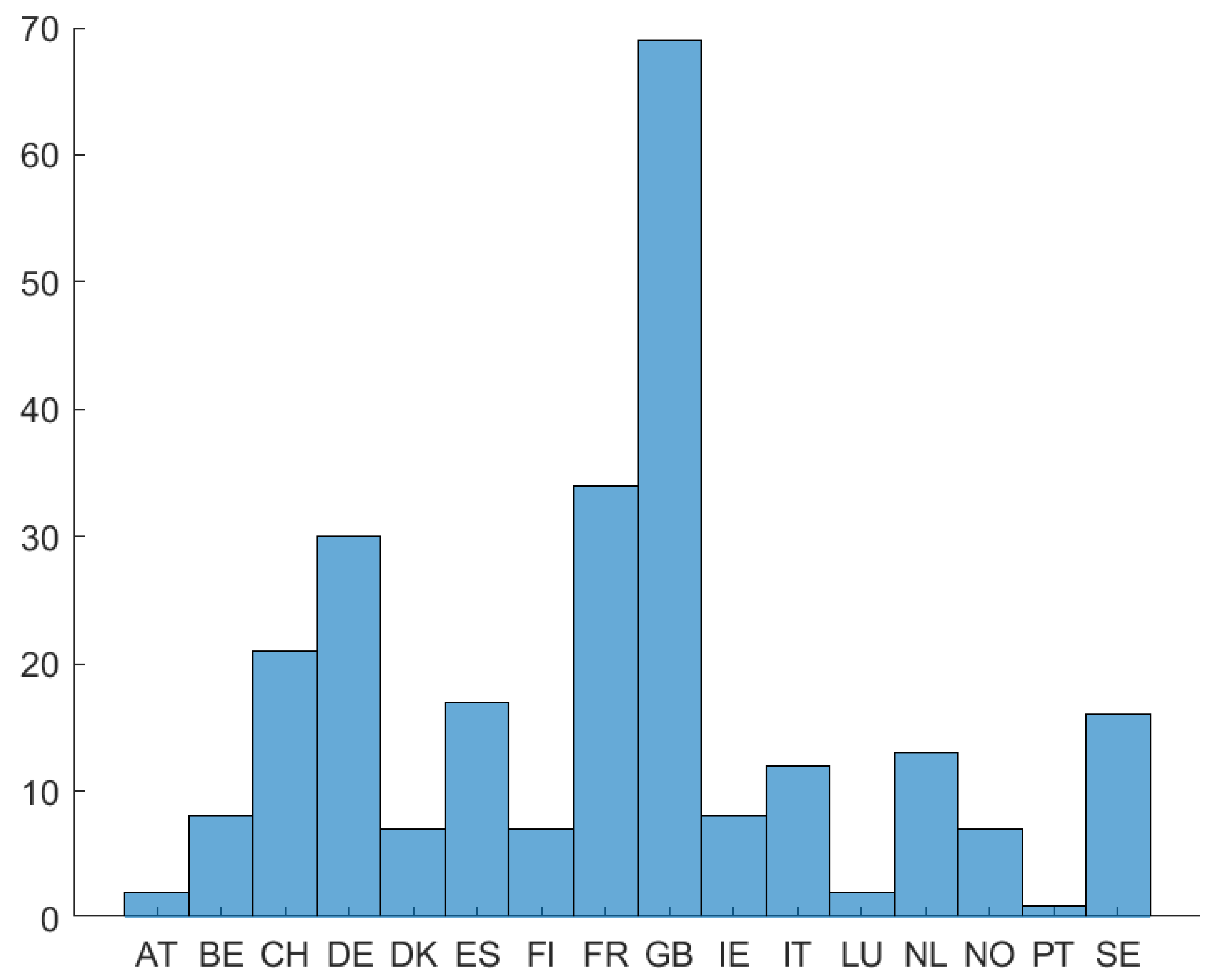
Country Code	Country	No. of Firms
AT	Austria	2
BE	Belgium	8
CH	Switzerland	21
DE	Germany	30
DK	Denmark	7
ES	Spain	17
FI	Finland	7
FR	France	34
GB	Great Britain	69
IE	Ireland	8
IT	Italy	12
LU	Luxembourg	2
NL	Netherlands	13
NO	Norway	7
PT	Portugal	1
SE	Sweden	16

Source: S&P Global and authors.

and

Table A11. Sectors.

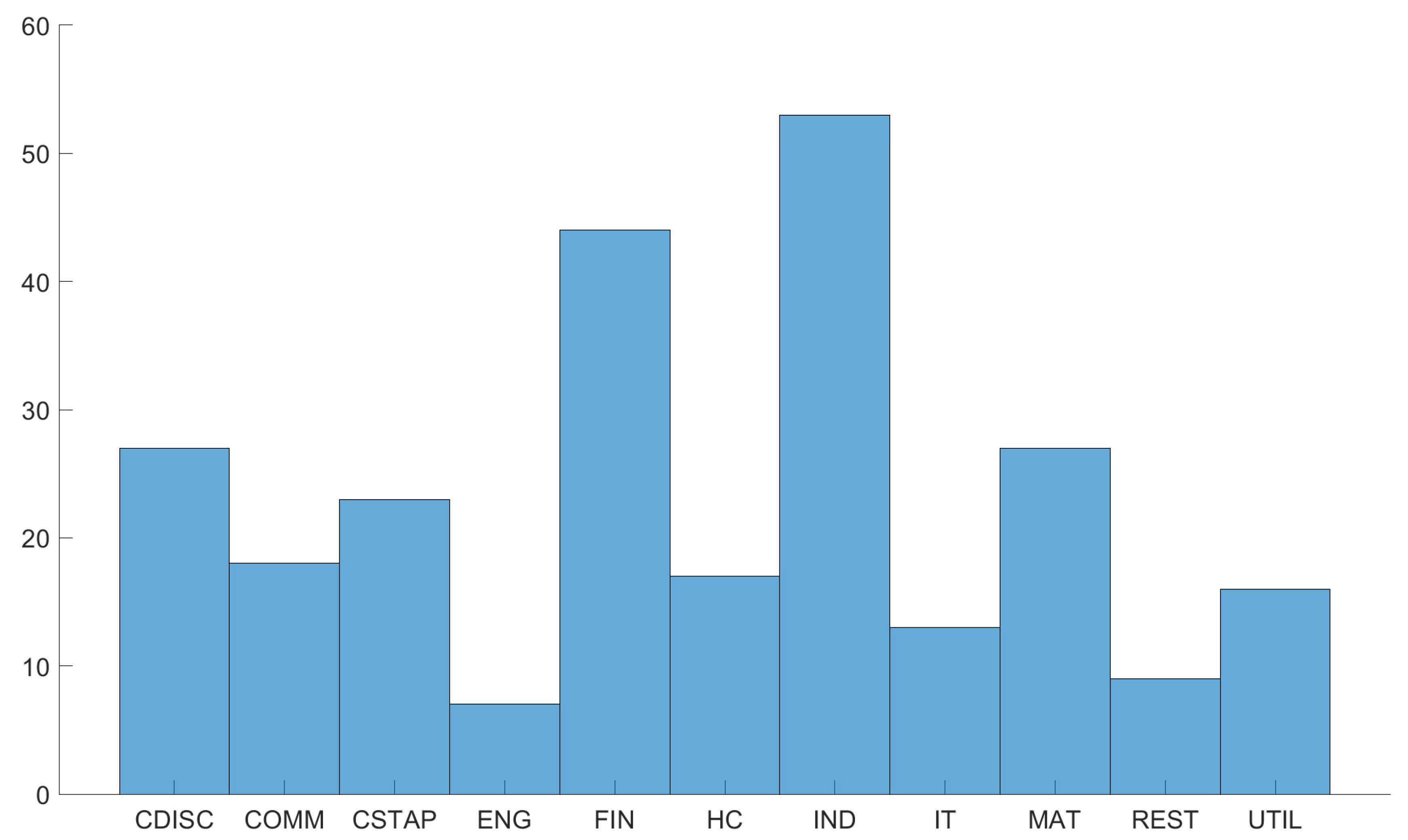
Sector Code	Sector	No. of Firms
CDISC	Consumer Discretionary	27
COMM	Communication Services	18
CSTAP	Consumer Staples	23
ENG	Energy	7
FIN	Financials	44
HC	Healthcare	17
IND	Industrials	53
IT	Information Technology	13
MAT	Materials	27
REST	Real Estate	9
UTIL	Utilities	16

Source: S&P Global and authors.

. From Figure 1, we can see that most of the firms in our data are from Great Britain, followed by France, Germany, and Switzerland. The least represented ones in the sample are Austria, Luxemburg, and Portugal. In our analysis, we considered the subsample of southern countries consisting of France, Spain, Italy, and Portugal. This subsample is largely led by France and Spain. Figure 2 shows that we have many firms from the Industrials and Financials sectors, followed by the Consumer Discretionary and Materials sectors. The least represented ones are the Energy and Real Estate sectors.

In Figure 3, we present the time series plot of the returns of all 254 stocks in our sample. As we can see, there are some positive and negative outliers in each series. The econometric model we discussed in Section 3 considers these outliers when modeling the returns. In Figure 4, we present the boxplots of the descriptive statistics of the return series. For example, the subfigure that corresponds to the mean shows the boxplot of the vector containing the means of each return series. In this figure, we can see that the average return for half of the stocks is slightly positive, between 0 and 0.00005. There are some return series that have relatively higher standard deviations. When we look at the skewness, we see that most series are negatively skewed and some series have strong negative skewness. Finally, as expected, the kurtosis is quite high, attracting attention to the fat tails of the return distributions.

In Figure 5, we present the histograms of the ESG ratings for all the firms and years, as well as year by year. From the pooled ESG ratings, we can see that the distribution is bi-modal and there is about a 40–45-point difference between the two modes. When we look at the histogram by years, we see that in the higher end of the distribution, the number of firms with high ESG ratings declined over the years. The numbers were especially high in 2016 and 2017, and after that, they declined. In the lower tail with ESG ratings of less than 30, we also see that the number of firms declined in 2021. On the other hand, we see an increasing trend over the years for the mid-range ESG ratings. For example, in the 40–50 range, we see that the number of firms increased. We can also say that with COVID-19, the number of firms in the mid-range increased. This means that some firms in the lower tail started to invest in ESG-related activities more, while some firms in the higher tail engaged less in ESG-related activities.

Our econometric model contains interaction terms, and hence, when evaluating the partial effects of the regressors, we need to know their sample means. In

Table 2. Averages of the regressor variables by the location of the firms.

	Beta	ESG	Solvency R.
All firms	0.9744	56.1548	35.1390
Southern	1.0489	68.7552	27.9963
Non-southern	0.9493	51.9105	37.5450

and

Table 3. Averages of the regressor variables by the sector of the firms.

	Beta	ESG	Solvency R.
COMM	0.7601	56.7778	33.9336
CDISC	1.0899	55.4444	42.4017
CSTAP	0.6300	48.9275	39.4335
ENG	1.0837	53.4286	45.4547
FIN	1.1801	58.4356	16.6283
HC	0.7450	57.6373	47.9136
IND	1.0494	50.8899	31.4282
IT	1.1006	58.7949	43.4659
MAT	1.1212	60.4444	47.6497
REST	0.7339	50.5556	52.4499
UTIL	0.6825	71.5938	25.5615

Note: The abbreviations and corresponding sector names are given in Table A11 in Appendix A.

, we present the averages of the regressors by country and by sector. In Table 2, we see that in southern countries’ (France, Italy, Spain, Portugal) firms are running higher risks compared to the S&P 350 Europe Index, as the average beta is above 1. On the other hand, in the non-southern countries, the average beta is 0.9493. We can see that the average ESG rating is higher for the firms in southern countries, which is very likely due to the investments in sustainable forms of energy. The solvency ratios of the firms in southern countries are much lower compared to the non-southern ones. When we look at the betas in Table 3, we see that the Consumer Discretionary, Energy, Financials, Information Technology, Industrials, and Materials sectors are running high risks, while the others are less risky than the S&P 350 Europe Index. Interestingly, the Consumer Staples sector has the lowest beta and also the lowest ESG rating. On the other hand, we see that the average ESG rating for the Utilities sector is much higher than the others. We can also note that the Financials and Utilities sectors are suffering in terms of solvency, while the Energy, Healthcare, Materials, and Real Estate sectors have high solvency ratios. From these tables, it is not possible to make conclusions on whether high solvency reduces the beta or higher ESG rating causes less risk.

5. Results

In this section, we start with comments on the estimates of the volatility models focusing on the asymmetry coefficients. Later, we turn to the fixed effects regressions and discuss the impact of ESG ratings on the asymmetry coefficients.

5.1. Asymmetry Coefficients

The coefficients for the asymmetric effects and leverage effects obtained from the AGARCH, NAGARCH, GJR-GARCH, and SVL models are presented as histograms in Figure 6. In these histograms, the bars are colored differently for each year, and for any given year, there are 254 asymmetry coefficients. It should be highlighted that in the AGARCH, NAGARCH, and GJR-GARCH models, the asymmetric effects occur if the parameter estimate is positive. With the SVL model, the leverage effects occur if the parameter estimate is negative. As Stavroyiannis (2018) notes, the asymmetric effects and leverage effect parameter with the wrong sign might indicate that the stock is a “safe haven” in times of crisis. As we can see from the figure, there are stocks for which the coefficient has the wrong sign for every model.

In Figure 6, we can see that AGARCH estimates for the asymmetric effect coefficient are distributed as a bell-shaped curve with a peak around zero. When we look at the bars in each year, we see that the asymmetry coefficient distribution is more negatively skewed in the year 2020, compared to other years. This is most likely due to the uncertainty that the COVID-19 pandemic brought to the finance world. In 2021, the distribution of the asymmetry coefficients became similar to how it was before the COVID-19 pandemic. A similar behavior is observed with GJR-GARCH coefficients.

When we look at the NAGARCH estimates of the asymmetry parameter, we see that the distribution has two peaks. One is around zero and the other one is around 1.5. We can see again that in the year 2020, the asymmetry coefficients were more negatively skewed. The histograms for the SVL model are telling a slightly different story, that in 2016, the leverage effect parameters were more positively skewed, similar to the year 2020. This was noticeable to some extent with the NAGARCH model as well.

Bekiros et al. (2017) and Bollerslev and Zhou (2006) discuss that these coefficients can be very model-dependent. Indeed, for the same data and time period, while one model shows small asymmetry coefficients, the other model could show large ones. In addition, the best-fitting model could change over the years. For instance, for a specific series, for the returns of a certain year, GJR-GARCH may be the best fit, while for the next year, the SVL model performs better.

Table 4. Model performance comparison, based on in-sample volatility estimates.

Years	GJR-GARCH	AGARCH	NAGARCH	SVL
2016	0.1496	0.2598	0.1063	0.4843
2017	0.2559	0.1496	0.1181	0.4764
2018	0.1772	0.1772	0.1024	0.5433
2019	0.2362	0.1378	0.1142	0.5118
2020	0.2205	0.3346	0.0787	0.3661
2021	0.2638	0.1299	0.1181	0.4882

Note: This table shows the root-mean-squared error between the estimated volatilities and squared residuals for each model. Squared returns or residuals can be used for model comparison purposes (see Moreira and Muir 2017; Becker and Leschinski 2021).

shows the proportions for which a certain model was fitting the volatility of a series the best based on the comparison of the volatility estimates with squared residuals. The comparison used the root-mean-squared error (RMSE) as a metric for the distance. We can see that most of the time, the SVL model was fitting the series best, which is in general followed by GJR-GARCH. The SVL model had its worst performance for the year 2020, opposite the AGARCH model, which performed the best in 2020.

In the next subsection, we discuss the results of the fixed effects regressions following the Arellano–Bond method. In these regressions, we fixed a certain volatility model and focused on the impact of ESG ratings. As we discussed, a certain volatility model does not fit the data of all the stocks in all these years well. This brings a limitation to our study that we may not be dealing with the best-fitting volatility model for each stock and year in these fixed effects regressions. If we were to proceed by only focusing on the stocks with the best-fitting volatility models, we would end up with unbalanced panel data and very few observations in some clusters.

5.2. The Impact of ESG Ratings

In this section, we discuss the results of the panel data regressions. We keep our focus on the Arellano–Bond estimator applied to the variables weighted by the standard errors of the dependent variable, i.e., the asymmetric effects or leverage effect coefficient from the volatility model. In

Table 5. AB-GLS estimation results for all models, Part I.

AB-GLS	AGARCH			NAGARCH
	All Firms	Southern	Non-Southern	All Firms	Southern	Non-Southern
.Lag1	−0.10829 **	0.02209	−0.14772 ***	−0.01884 ***	0.06169	−0.01953 ***
Beta	0.00127	−0.00024	0.00132	−1.39361 *	−0.26217	−1.48509 *
ESG	0.00000	0.00002	0.00000	−0.00456 *	−0.00402	−0.00473 *
Solvency R.	−0.00003	0.00008	−0.00003	0.05820 *	0.01749	0.06152 *
Beta.ESG	−0.00002	−0.00001	−0.00002	0.01814 *	0.00832	0.01951 *
ESGSolv	0.00000	−0.00000	0.00000	−0.00062 *	−0.00041	−0.00067 *
COVID	0.00285 *	−0.00916 *	0.00305	−1.11383 *	−1.15177 *	−0.11889
ESG.COVID	−0.00002	0.00004	−0.00002	0.01782 *	0.01073	0.00176
Beta.COVID	0.00421 ***	0.00740 **	0.00469 ***	0.26539	0.13665	0.59359
SolvCOVID	−0.00006 ***	0.00008	−0.00008 ***	−0.01599 *	0.01528 **	−0.02699 *
N. obs.	1016	256	760	1016	256	760
N. groups	254	64	190	254	64	190
Ftest_Pval	0.00000	0.00000	0.00000	0.00000	0.00000	0.00000
BC.MEM. ESG	0	0	0	−0.00867	0	−0.01136
AC.MEM. ESG	0	0	0	0.00915	0	−0.00960

Note: AB-GLS is the Arellano–Bond estimation method where the variables are weighed by the standard error of the dependent variable. *, **, *** denote significance at 10%, 5% and 1% significance levels. BC.MEM and AC.MEM indicate marginal effect at sample means before and after COVID-19.

and

Table 6. AB-GLS estimation results for all models, Part II.

AB-GLS	GJR-GARCH			SVL
	All Firms	Southern	Non-Southern	All Firms	Southern	Non-Southern
.Lag1	−0.00857	0.11726	−0.00244	−0.06767 *	0.00277	−0.10420 **
Beta	0.03774	0.01383	0.06094	−0.35202 ***	−0.62741 ***	−0.27979 ***
ESG	−0.00332 ***	−0.00044 *	−0.00437 ***	−0.00815 ***	−0.00797 ***	−0.00757 ***
Solvency R.	−0.00047	−0.00041	0.00068	−0.00244	−0.00653	−0.00218
Beta.ESG	0.00245 **	0.00013	0.00033	0.00334 **	0.00717 ***	0.00202
ESGSolv	−0.00002	0.00001	0.00005 ***	0.00007 *	0.00012	0.00005
COVID	−0.15843	−0.09645	−0.03549	−0.02563	0.01659	0.03359
ESG.COVID	0.00267 *	0.00065	0.00338 ***	0.00136	−0.00243	0.00146
Beta.COVID	−0.02997	0.08343 ***	0.02110	−0.04560	0.11494	−0.11083 *
SolvCOVID	0.00486 ***	−0.00001	−0.00171 **	−0.00086	0.00053	−0.00067
N. obs.	1016	256	760	1016	256	760
N. groups	254	64	190	254	64	190
Ftest_Pval	0.00000	0.00000	0.00000	0.00000	0.00000	0.00000
BC.MEM. ESG	−0.00093	−0.00044	−0.00249	−0.00244	−0.00045	−0.00757
AC.MEM. ESG	0.00174	−0.00044	0.00089	−0.00244	−0.00045	−0.00757

Note: AB-GLS is the Arellano–Bond estimation method where the variables are weighed by the standard error of the dependent variable. *, **, *** denote significance at 10%, 5% and 1% significance levels. BC.MEM and AC.MEM indicate marginal effect at sample means before and after COVID-19.

, we present the coefficients from the Arellano–Bond estimator for the AGARCH, NAGARCH, GJR-GARCH, and SVL models. It is important to remember here that an increase in the dependent variable means higher asymmetry for the AGARCH, NAGARCH, and GJR-GARCH models, while it means less leverage effect in the SVL model.

In Table 5, when we look at the estimation results for the AGARCH coefficients, we see that there are many insignificant coefficients. For the whole sample and for the non-southern countries, we can see that the first lag of the asymmetry coefficient is significant and negative. When considering the whole sample, we see that a higher beta increases the asymmetry only in the COVID-19 pandemic period, i.e., after 2020. For the whole sample and for non-southern countries, higher solvency ratios reduce asymmetry only in the COVID-19 pandemic period. Focusing on the COVID-19 impact, we found that the marginal effect evaluated at the sample mean is 0.004968. This means that in the COVID-19 pandemic period, the asymmetry coefficient increased. The estimations are most likely picking up the positive jump in the asymmetry coefficients in 2020. Interestingly, for the AGARCH model, the coefficients of the ESG ratings or any of its interactions are not significant; therefore, we say that the marginal effect of ESG ratings is zero9.

In the same table, we have more significant coefficients with the NAGARCH model. When we consider the whole sample and non-southern countries, we found again that the autoregressive coefficient is negative and significant. The partial effect of the beta increases with the ESG ratings. This means that the asymmetry coefficient for the riskier firms rose further if their ESG ratings were high. This could mean that for the riskier firms, having high ESG ratings was seen as an additional risk factor, and therefore, the investors were cautious about any negative shocks for these firms. This finding is in line with Bae et al. (2021), that if the firms try to hide their unfavorable/risky positions, this may suppress the good impact of ESG ratings on the financial risk. The partial effect of the solvency ratio was less for higher ESG ratings and after COVID-19. Therefore, when the firms engaged in ESG-related activities more, their solvency was reducing the asymmetry effect less. The marginal effect of the solvency ratio at the sample mean was 0.00739, indicating that the firms with higher solvency ratios had higher asymmetry coefficients. In particular, we see that for the southern countries, higher solvency ratios during the COVID-19 pandemic meant higher asymmetry coefficients. It seems that in the southern countries, COVID-19 reduced the asymmetry coefficients, but this reduction was less for high-solvency firms. Contrary to this, in non-southern countries, higher solvency ratios during COVID-19 are associated with smaller asymmetry coefficients. When we focus on the ESG ratings, we see that the coefficient of ESG ratings is negative and its partial effect decreases further with the solvency ratio, but increases with the beta and during the COVID-19 period. This would imply that for firms with high solvency ratios, ESG ratings reduce asymmetry coefficients further. However, when the firms are riskier than the market, this impact is lessened. The marginal effect of ESG ratings evaluated at the sample mean is -0.00867 before the COVID-19 pandemic and 0.00915 during the pandemic. This indicates that before the COVID-19 pandemic, engaging in ESG-related activities reduced the asymmetry behavior, but afterwards, it was perceived as an additional risk by the investors, inducing further asymmetry behavior in volatility. While for the southern countries, the marginal effect of ESG ratings was zero, for the non-southern countries, it was negative both before and after COVID-19.

In Table 6, we give the AB-GLS estimation results for the GJR-GARCH and SVL models, which fit the data in general better than the AGARCH and NAGARCH models. This is also highlighted in Table 4. When we look at the results for the GJR-GARCH model, we see that the autoregressive coefficient is no longer significant. The partial effect of beta depends on the ESG ratings, meaning that for firms with higher ESG ratings, being riskier than the market increases the asymmetry coefficient further. Again, this result confirms that investors perceive higher ESG ratings as additional risk when the firms are already riskier than the market. Higher solvency ratios increase the asymmetry behavior in volatility only in the COVID-19 period. The partial effect of ESG ratings increases with beta and in the COVID-19 period. The marginal effect of ESG ratings at the sample means is −0.00093 before COVID-19 and 0.00174 after it. This impact is more distinct for the non-southern firms.

In the same table, when we look at the SVL model results, we see that the autoregressive coefficients are significant for the whole sample and for non-southern countries. A higher beta is associated with stronger leverage effects. For the whole sample and for southern countries, this impact is reduced as the ESG ratings increase, but it is more pronounced in the non-southern countries. The partial effect of the solvency ratio is not significant in all the samples. When we focus on the ESG ratings, we see that the marginal effects at the sample mean are the same before and after COVID-19. It seems that higher ESG ratings are associated with higher leverage effects. In addition, we see that the partial effect of ESG ratings depends positively on the betas. This means that higher ESG ratings imply higher asymmetry behavior for low-risk firms. For high-risk firms, maintaining high ESG ratings actually helps reduce the leverage effect. This result seems to be in a different direction from the findings with the NAGARCH and GJR-GARCH models.

In

Table 7. AB-GLS results, by sector.

Sectors	ESG	Beta.ESG	ESG.Solv.	ESG.Covid	Obs./Gr.	MEM. of ESG
AGARCH: CSTAP ENG IND IT MAT REST UTIL	. −0.00013 ** 0.00038 *** 0.00013 * −0.00028 ** −0.00012 ** 0.00023 ** .	. . . . 0.00024 ** . −0.00043 ** 0.00046 ***	. . . . . . . .	. . . . 0.00043 *** . . .	. 92/23 28/7 212/53 52/13 108/27 36/9 64/16	. −0.00013 0.00038 0.00013 −0.00002/0.00041 −0.00012 −0.00009 0.00031
NAGARCH: CDISC HC IND IT MAT	. −0.01730 * . 0.00158 * −0.04358 *** −0.01045 *	. . 0.02484 ** . 0.03469 *** −0.03264 *	. −0.00057 *** . . . 0.00122 *	. . . . . .	. 108/27 68/17 212/53 52/13 108/27	. −0.04147 0.01851 0.00158 −0.00540 0.01109
GJR-GARCH: ENG IT UTIL	. . . −0.00709 ***	. 0.00626 *** 0.00186 ** .	. −0.00018 * . 0.00029 ***	. . . .	. 28/7 52/13 64/16	. −0.00139 0.00205 0.00032
SVL: COMM CDISC CSTAP ENG FIN HC IND REST UTIL	. −0.01129 ** −0.00757 *** . −0.01435 * −0.01005 *** . −0.01267 *** −0.01126 ** −0.00855 *	. 0.01365 ** . 0.00833 * . 0.00771 ** −0.01054 ** 0.00456 * 0.01995 * .	. . 0.00011 ** . . . 0.00015 * . . .	. . . . . . . . . .	. 72/18 108/27 92/23 28/7 176/44 68/17 212/53 36/9 64/16	. −0.00091 −0.00291 0.00525 −0.01435 −0.00095 −0.00067 −0.00788 −0.00791 −0.00855

Note: AB-GLS is the Arellano–Bond estimation method where the variables are weighed by the standard error of the dependent variable. *, **, *** denote significance at 10%, 5% and 1% significance levels. MEM indicates marginal effect at sample means. If the MEM is different before and after COVID-19, both numbers are reported, separated with a “/”.

, we present the estimation results by sector. Following the same pattern as before, the AB-GLS method was applied to the four volatility models, but restricting the sample to only a specific sector. When presenting the results, we maintained our focus on the coefficients of the ESG rating variable and its interactions with other variables. We calculated the marginal effects at the sample means only using the statistically significant coefficients.

For the AGARCH model, the marginal effect of ESG ratings at the sample means suggests that higher ESG ratings reduce the asymmetry behavior in volatility in the Consumer Staples, Materials, and Real Estate sectors, while increasing it in the Energy, Industrials, Information Technology (in particular, after COVID-19), and Utilities sectors. The finding for the Energy sector is consistent with Lundgren et al. (2018), since they found that European renewable energy stocks may bear more risks. For the NAGARCH model, for the Consumer Discretionary and Information Technology sectors, the marginal effect of ESG ratings is negative, while for the Healthcare, Industrials, and Materials sectors, it is positive. For the GJR-GARCH model, only in the Energy sector, the marginal effect of ESG ratings is negative, while in the Information Technology and Utilities sectors, it is positive. Finally, for the SVL model, we see that only for the Consumer Staples sector, higher ESG ratings mean less leverage effect, while for the rest of the sectors, the marginal effects of ESG ratings are negative. We also see that only in the AGARCH model and Information Technology sector, the partial effect changes in the COVID-19 period, reversing the sign of the marginal effect of ESG ratings at the sample means.

When we look at the summary of these results in

Table 8. Summary of results by sector for the AB-GLS approach.

Sectors	ESG Ratings Increase Asymmetry/Leverage	ESG Ratings Decrease Asymmetry/Leverage
COMM	SVL	-
CDISC	SVL	NAGARCH
CSTAP	-	AGARCH, SVL
ENG	AGARCH, SVL	GJR-GARCH
FIN	SVL	-
HC	NAGARCH, SVL	-
IND	AGARCH, NAGARCH, SVL	-
IT	AGARCH, GJR-GARCH	AGARCH(vs), NAGARCH
MAT	NAGARCH	AGARCH
REST	SVL	AGARCH(vs)
UTIL	AGARCH, GJR-GARCH, SVL	-

Note: If the marginal impact is less than 0.0001, we denote it with a “vs” to indicate that it is very small. AB-GLS is the Arellano–Bond estimation method where the variables are weighed by the standard error of the dependent variable.

, we see that for the Communications, Financials, Healthcare, Industrials, and Utilities sectors, the findings suggest that higher ESG ratings are associated with higher asymmetry/leverage. The findings for the Financials sector are not consistent with the study of Sonnenberger and Weiss (2021), since for the insurance firms, they found that higher ESG ratings were linked to lower tail risk. On the other hand, for the Consumer Staples sector, we found the opposite relation. For the rest of the sectors in Table 8, there is controversy between the findings for these models. However, as Table 4 indicates, the SVL model had a better fit about half of the time in the samples. Therefore, when there is controversy between SVL and the other models, perhaps more weight could we given to the SVL results. Hence, it could be that in the Consumer Discretionary, Energy, and Real Estate sectors, ESG ratings are associated with higher asymmetry/leverage.

6. Robustness Analysis

In fixed effects regressions, the robust standard errors option is used to at least asymptotically mitigate the problem of heteroscedasticity and serial correlation10 (Arellano et al. 1987). Therefore, we estimated the model in Equation (9) via the Arellano–Bond approach using the robust standard errors, without weighting the variables with the standard errors of the asymmetry coefficients. However, we found mostly insignificant coefficients. This was most likely due to the fact that the robust standard errors option works asymptotically, assuming a large number of clusters. Perhaps given the number of stocks in our dataset, the robust standard errors could not accommodate the heteroscedasticity caused by using an estimated dependent variable. We do not report these results in the paper, as there was no gain from these estimations.

In terms of specifications to eliminate possible reverse causality, we tried fixed effects regressions (both regular and GLS versions) with lagged regressors as in Equation (8). As mentioned by Bellemare et al. (2017), this approach is also quite popular. However, Reed (2015) suggests this approach does not resolve the biases in the point estimates and in the inferences caused by reverse causality issues. Therefore, we discarded these results.

To handle the possible reverse causality issue, we also tried the lagged first difference (LFD) method, which was proposed by Allison (2009). As with the Arellano–Bond method, using only the robust standard errors yielded a few significant coefficients. Hence, we weighed the variables with the standard errors of the asymmetry coefficients. In

Table A1. LFD-GLS estimation results for all models, Part I.

LFD-GLS	AGARCH			NAGARCH
	All Firms	Southern	Non-Southern	All Firms	Southern	Non-Southern
Beta	0.00032	0.00738 ***	−0.00022	1.02073 **	0.84128	1.01664 **
ESG	−0.00000	−0.00005 *	−0.00000	0.00310 **	−0.00122	0.00314 **
Solvency R.	0.00000	−0.00022 ***	0.00002	−0.04138 ***	−0.05175	−0.04138 ***
Beta.ESG	0.00000	−0.00006	0.00001	−0.01336 **	−0.00971	−0.01324 **
ESGSolv	0.00000	0.00000	−0.00000	0.00045 ***	0.00067	0.00045 ***
COVID	0.00082	−0.01175	0.00170	0.42901	1.28019	0.02021
ESG.COVID	0.00001	0.00008	−0.00000	−0.00705 *	0.00147	0.00209
Beta.COVID	−0.00549 ***	0.00072	−0.00630 ***	−0.30962	-1.21798 *	−0.33188
SolvCOVID	−0.00006 *	−0.00001	−0.00005	0.01146 **	−0.00464	0.01259 *
N. obs.	1016	256	760	1016	256	760
R2	0.0944	0.1350	0.1028	0.3433	0.0556	0.3493
Ftest_Pval	0.00000	0.00000	0.00000	0.00000	0.00000	0.00000
BC.MEM. ESG	0	−0.00005	0	0.00589	0	0.00747
AC.MEM. ESG	0	−0.00005	0	−0.00115	0	0.00747

Note: LFD-GLS is the lagged first difference estimation method where the variables are weighed by the standard error of the dependent variable. *, **, *** denote significance at 10%, 5% and 1% significance levels. BC.MEM and AC.MEM indicate marginal effect at sample means before and after COVID-19.

and

Table A2. LFD-GLS estimation results for all models, Part II.

LFD-GLS	GJR-GARCH			SVL
	All Firms	Southern	Non-Southern	All Firms	Southern	Non-Southern
Beta	0.04087	−0.02972	−0.00612	0.07064	0.47665 **	−0.00181
ESG	0.00173 ***	0.00011	0.00201 ***	0.00332 *	0.00609 *	0.00255
Solvency R.	−0.00144	0.00147	−0.00226	0.00427 **	−0.00319	0.00492 **
Beta.ESG	−0.00209 *	0.00032	−0.00073	−0.00150	−0.00749 **	−0.00007
ESGSolv	0.00003	−0.00002	0.00001	−0.00003	0.00000	−0.00003
COVID	0.18039 ***	−0.14648	0.16638 ***	0.15451	−0.01744	0.13012
ESG.COVID	0.00063	0.00148	0.00075	−0.00189 *	0.00059	−0.00124
Beta.COVID	−0.14185	0.02061	−0.18603	0.07204	0.05346	0.07612
SolvCOVID	−0.00424 ***	0.00000	−0.00224	−0.00003	−0.00209	0.00014
N. obs.	1016	256	760	1016	256	760
R2	0.4087	0.0240	0.4206	0.0841	0.0884	0.0927
Ftest_Pval	0.00000	0.00310	0.00000	0.00000	0.00530	0.00000
BC.MEM. ESG	−0.00031	0	0.00201	0.00332	−0.00177	0
AC.MEM. ESG	−0.00031	0	0.00201	0.00143	−0.00177	0

Note: LFD-GLS is the lagged first difference estimation method where the variables are weighed by the standard error of the dependent variable. *, **, *** denote significance at 10%, 5% and 1% significance levels. BC.MEM and AC.MEM indicate marginal effect at sample means before and after COVID-19.

in Appendix A, we present the LFD-GLS method results for different volatility models.

For the AGARCH model and for the whole sample, the LFD-GLS results suggest that higher betas and higher solvency rates are associated with lower asymmetry during the COVID-19 period. This means that for riskier firms and for firms with higher solvency rates during the COVID-19 time, the investors’ reaction to negative news was more stable. The ESG ratings affect negatively the asymmetry effect only in the southern countries and to a small extent.

For the NAGARCH model, the findings are different. The partial effect of the beta is reduced for higher ESG ratings, and the marginal effect at the sample means is 0.27051. This means that for riskier firms, the asymmetry coefficient is higher on average, but if the riskier firms engage more in ESG-related activities, this effect is reduced. This finding is consistent with Bae et al. (2021), that higher ESG ratings may reduce the stock price crash risk. The partial effect of solvency ratios is negative, and it increases with the ESG ratings and during COVID-19. The marginal effects at the sample means are −0.01611 and −0.00465 for the whole sample before and after COVID-19, respectively. Since the solvency ratio is an inverse measure of the financial leverage, we can say that this is some empirical evidence to support the relation of financial leverage to asymmetric effects, as mentioned in Christie (1982) and Choi and Richardson (2016). The partial effect of ESG ratings depends negatively on the betas and positively on the solvency ratios. During COVID-19 also, this partial effect is reduced. The marginal effect of ESG ratings at the sample means is positive before COVID-19 and negative afterwards. This result tells a different story compared to the AB-GLS results, that before COVID-19, the ESG-related investments were perceived as an additional risk by the investors, but during COVID-19, this perhaps reduced their concerns about possible negative news. When considering only southern countries, we did not find any significant impact, but for the non-southern countries, the results were similar to the whole sample ones.

When we focus on the GJR-GARCH results, we noticed that the partial effect of the beta is negatively related to the ESG ratings. We also see that solvency ratios affect asymmetry negatively only in the COVID-19 period. The marginal effect of the COVID-19 dummy variable evaluated at the sample mean of the solvency ratio is 0.09605, which means that on average, the impact of COVID-19 on the asymmetry coefficient was positive. We found for the whole sample that the marginal effect of ESG ratings is small and negative, while for the non-southern countries, it is slightly larger in magnitude and positive. The latter result implies that engaging in ESG-related activities increased the asymmetry behavior for non-southern firms.

In the results for the SVL model, we see that while the beta does not have an impact on the leverage coefficients, higher solvency ratios are linked to lower leverage effects11. The partial effect of ESG ratings is 0.00332 before COVID-19 and 0.00143 afterwards, meaning that higher ESG ratings mean lower leverage effects. Interestingly, the sign reverses for the southern countries, since there, the partial effect of ESG ratings depends on the riskiness of the firms.

In

Table A3. LFD-GLS results, by sector.

Sectors	ESG	Beta.ESG	ESG.Solv.	ESG.Covid	Nr. Obs.	MEM. of ESG
AGARCH: IND	. −0.00016 ***	. .	. 0.00001 ***	. .	. 212	. 0.00015
NAGARCH: CDISC CSTAP FIN IND UTIL	. 0.03599 *** . −0.00844 * −0.00226 *** .	. −0.03178 ** . . −0.00701 *** −0.02342 *	. . 0.00119 * . 0.00029 *** .	. . . . . .	. 108 92 176 212 64	. 0.00135 0.04693 −0.00844 −0.00050 −0.01598
GJR-GARCH: IND IT	. . 0.00177 *	. . .	. 0.00014 * .	. . .	. 212 52	. 0.00439 0.00177
SVL: COMM CDISC ENG HC IND IT	. . . . . 0.01424 *** .	. −0.00901 * 0.00624 ** . 0.01334 ** . .	. . . −0.00083 * −0.00036 *** −0.00045 ** 0.00049 *	. . . . 0.00727 * . .	. 72 108 28 68 212 52	. −0.00685 0.00680 −0.03773 −0.00731/0.00004 0.00009 0.02129

Note: LFD-GLS is the lagged first difference estimation method where the variables are weighed by the standard error of the dependent variable. *, **, *** denote significance at 10%, 5% and 1% significance levels. MEM indicates marginal effect at sample means. If the MEM is different before and after COVID-19, both numbers are reported, separated with a “/”.

in the Appendix A, we see that for the AGARCH model, the marginal effect of ESG ratings at the sample mean is positive for the Industrials sector. The NAGARCH model results suggest that the marginal effect of ESG ratings is positive for the Consumer Discretionary and Consumer Staples sectors and negative for the Financials, Industrials, and Utilities sectors. For the GJR-GARCH model, the marginal effect of ESG ratings is positive for the Industrials and Information Technology sectors. Finally, for the SVL model, the marginal effects of ESG ratings at the sample means are negative for the Communications, Energy, and Healthcare sectors, while they are positive for the Consumer Discretionary, Industrials, and Information Technology sectors. For the SVL model, a negative impact on the leverage coefficient means that the leverage effect is higher. These findings are summarized in

Table 9. Summary of results by sector for the LFD-GLS approach.

Sectors	ESG Ratings Increase Asymmetry/Leverage	ESG Ratings Decrease Asymmetry/Leverage
COMM	SVL	-
CDISC	NAGARCH	SVL
CSTAP	NAGARCH	-
ENG	SVL	-
FIN	-	NAGARCH
HC	SVL	SVL(vs)
IND	AGARCH, GJR-GARCH	NAGARCH, SVL(vs)
IT	GJR-GARCH	SVL
MAT	-	-
REST	-	-
UTIL	-	NAGARCH

Note: If the marginal impact is less than 0.0001, we denote it with a “vs” to indicate that it is very small. LFD-GLS is the lagged first difference estimation method where the variables are weighed by the standard error of the dependent variable.

. We find that in the Communications, Consumer Staples, Energy, and Healthcare sectors, higher ESG ratings are associated with increased asymmetry/leverage. On the other hand, in the Financials and Utilities sectors, the effect is reversed. If we were to favor the SVL model when there are different results with different volatility models, then perhaps we could also infer that for the Consumer Discretionary and Information Technology sectors, higher ESG ratings could reduce asymmetry/leverage. We cannot make such an extrapolation with the Industrials sector as the impact for the SVL model is relatively small.

Finally, we considered a comparison of the overall findings with the AB-GLS and LFD-GLS methods for the marginal effects of ESG ratings evaluated at the sample means. We present the results in

Table 10. Comparing results with the AB-GLS and LFD-GLS models.

Sectors	AB-GLS	LFD-GLS
COMM	increase	increase
CDISC	increase (?)	decrease (?)
CSTAP	decrease	increase
ENG	increase (?)	increase
FIN	increase	decrease
HC	increase	increase
IND	increase	not clear
IT	not clear	decrease (?)
MAT	not clear	no result
REST	increase (?)	no result
UTIL	increase	decrease

Note: AB-GLS and LFD-GLS represent the Arellano–Bond and lagged first difference methods, respectively. An increase/decrease indicates that higher ESG ratings are associated with higher/lower asymmetry or the leverage effect. A question mark “?” is added to indicate the cases where the results for SVL are reported, but keeping in mind that the results for some other volatility models are different. We report “not clear” when, for the volatility models other than SVL, we obtained contradictory results. Finally, we report “no result” if the coefficients were insignificant and the marginal effect could not be calculated.

. We can immediately notice that for the Communications and Healthcare sectors, both the AB-GLS and LFD-GLS methods indicate that higher ESG ratings are associated with higher asymmetry/leverage. It is also possible to extrapolate this relation for the Energy and Real Estate sectors, if we give higher weight to the results with the SVL model, which was fitting the data better most of the time than the other models. Finally, we also note such a relation for the Industrials sector based on the AB-GLS method. For the Consumer Discretionary, Consumer Staples, Financials, and Utilities sectors, we have contradictory results for the AB-GLS and LFD-GLS methods. Last but not least, the LFD-GLS method could be suggesting a negative relation between ESG ratings and asymmetry/leverage coefficients for the Information Technology sector, if we give higher weight to the results with the SVL model.

7. Conclusions

In this paper, we explored if maintaining higher ESG ratings can be associated with higher asymmetric effects or leverage effects in the volatility of stock returns. For this purpose, we used the daily returns of the S&P Europe 350 Index constituent stocks, along with their annual ESG ratings and solvency ratios for the period January 2016–December 2021. We acknowledge that our conclusions are only for the S&P Europe 350 Index, which consists of the most liquid European stocks, and for this time period. In terms of methodology, we applied the AGARCH, NAGARCH, GJR-GARCH, and SVL models to ARMA-filtered series and obtained the coefficients of asymmetric effects or leverage effects. The common characteristic of these volatility models is that they all have only one parameter that controls for the asymmetry. We then used the asymmetric effects and leverage effect coefficients as dependent variables in panel data regressions, where the independent variables were the betas, ESG ratings, solvency ratios, COVID-19 dummy variable, and their interactions. The heteroscedasticity problem caused by using estimated dependent variables was addressed by weighing the variables of the models with the standard error of the dependent variable. To avoid possible reverse causality issues, we used Arellano–Bond and lagged first difference estimators.

Since lagged first difference estimators could suffer from biases if the timing of the causality is misspecified, we focused on the Arellano–Bond estimator results. Our results in general indicate that a higher beta is associated with higher asymmetry and leverage effects. This effect is more pronounced for firms with high ESG ratings and during the COVID-19 period. In principle, this could mean that investors perceive it negatively if the firms are running high risks and at the same time engaging in ESG-related activities. We also found that solvency ratios are negatively related to the asymmetric behavior in volatility, although for some models, we found a positive relation. Since solvency ratios are related to firm leverage inversely, the finding suggests that firm leverage is associated with the asymmetry behavior of volatility. We also found partial evidence that high ESG ratings are associated with lower asymmetry before COVID-19, but with higher asymmetry after COVID-19. We also found that in the COVID-19 period, the asymmetry behavior in volatility was on average higher.

When we considered the marginal effects of ESG ratings in each sector with the Arellano–Bond estimation method, we can say that the impact of ESG ratings on the asymmetry behavior of volatility was positive for the Communications, Financials, Healthcare, Industrials, and Utilities sectors. We can also speculate to some degree the same relation with the Consumer Discretionary, Energy, and Real Estate sectors, if we consider that the SVL model fit the volatility best. When we cross-checked these results with the lagged first difference estimation method, we observed that only for the Communications and Healthcare sectors, the impact of ESG ratings on the asymmetry behavior was positive. This could be extrapolated to the Energy, Industrials, and Real Estate sectors, if we consider assigning more weight to the results for the SVL model.

The findings of this paper could be very useful to investors. On the one hand, in certain sectors, firms with high betas striving to maintain vigorous ESG-related activities could signal a higher asymmetric behavior of the volatility process, which could in turn mean strong reactions to negative news. Perhaps it could be a sign of green washing activity such that the firms try to conceal their riskiness behind the ESG ratings. On the other hand, our results suggested that the marginal effect of ESG ratings at the sample means was positive during the COVID-19 pandemic. This suggests that in risky times, engaging in ESG-related activities could be seen as an additional risk by the investors. The paper has also some valuable implications for practitioners. The positive marginal effect of ESG ratings on the asymmetric behavior suggests that in the face of a negative return shock, the volatility of a firm rises even higher if that firm has high ESG ratings. This could be related to the systemic risk literature, that firms with high risk and high ESG ratings could potentially contribute more to systemic risk and adversely affect the economies in the long run.

This paper can be extended in multiple ways. The data we considered focus primarily on blue-chip companies from developed European countries. These are the most liquid stocks from the European markets. Future research could be conducted to assess this phenomenon from the liquidity status of firms, i.e., less-liquid versus high-liquidity stocks. The expansion of the data to include also developing countries along with liquidity could generate interesting insights in the subject matter. Solvency ratios were the liquidity measure that gave us the highest possible number of stocks. Future investigations could consider other measures of liquidity or firm leverage if the dataset is expanded to include a substantially higher number of firms.

References

- Adrian, Tobias, and Hyun Song Shin. 2010. Liquidity and leverage. Journal of Financial Intermediation 19: 418–37. [Google Scholar] [CrossRef]
- Aharon, David Yechiam, and Yossi Yagil. 2019. The impact of financial leverage on the variance of stock returns. International Journal of Financial Studies 7: 14. [Google Scholar] [CrossRef]
- Allison, Paul D. 2009. Fixed Effects Regression Models. Thousand Oaks: SAGE Publications. [Google Scholar]
- Anderson, Theodore Wilbur, and Cheng Hsiao. 1981. Estimation of dynamic models with error components. Journal of the American Statistical Association 76: 598–606. [Google Scholar] [CrossRef]
- Arellano, Manuel. 1987. Computing robust standard errors for within-groups estimators. Oxford Bulletin of Economics and Statistics 49: 431–34. [Google Scholar] [CrossRef]
- Arellano, Manuel, and Stephen Bond. 1991. Some tests of specification for panel data: Monte carlo evidence and an application to employment equations. The Review of Economic Studies 58: 277–97. [Google Scholar] [CrossRef]
- Asai, Manabu, and Michael McAleer. 2011. Alternative asymmetric stochastic volatility models. Econometric Reviews 30: 548–64. [Google Scholar] [CrossRef]
- Asai, Manabu, Michael McAleer, and Jun Yu. 2006. Multivariate stochastic volatility: A review. Econometric Reviews 25: 145–75. [Google Scholar] [CrossRef]
- Bae, JinCheol, Xiaotong Yang, and Myung-In Kim. 2021. Esg and stock price crash risk: Role of financial constraints. Asia-Pacific Journal of Financial Studies 50: 556–81. [Google Scholar] [CrossRef]
- Balcilar, Mehmet, Riza Demirer, and Rangan Gupta. 2017. Do sustainable stocks offer diversification benefits for conventional portfolios? An empirical analysis of risk spillovers and dynamic correlations. Sustainability 9: 1799. [Google Scholar] [CrossRef]
- Becker, Janis, and Christian Leschinski. 2021. Estimating the volatility of asset pricing factors. Journal of Forecasting 40: 269–78. [Google Scholar] [CrossRef]
- Bekaert, Geert, and Guojun Wu. 2000. Asymmetric volatility and risk in equity markets. The Review of Financial Studies 13: 1–42. [Google Scholar] [CrossRef]
- Bekiros, Stelios, Mouna Jlassi, Kamel Naoui, and Gazi Salah Uddin. 2017. The asymmetric relationship between returns and implied volatility: Evidence from global stock markets. Journal of Financial Stability 30: 156–74. [Google Scholar] [CrossRef]
- Bellemare, Marc F., Takaaki Masaki, and Thomas B. Pepinsky. 2017. Lagged explanatory variables and the estimation of causal effect. The Journal of Politics 79: 949–63. [Google Scholar] [CrossRef]
- Black, Fischer. 1976. Studies of Stock Market Volatility Changes. Washington, DC: American Statistical Association Business and Economic Statistics Section. [Google Scholar]
- Bollerslev, Tim, and Hao Zhou. 2006. Volatility puzzles: A simple framework for gauging return-volatility regressions. Journal of Econometrics 131: 123–50. [Google Scholar] [CrossRef]
- Bollerslev, Tim, and Jeffrey M. Wooldridge. 1992. Quasi-maximum likelihood estimation and inference in dynamic models with time-varying covariances. Econometric Reviews 11: 143–72. [Google Scholar] [CrossRef]
- Bolton, Patrick, and Marcin Kacperczyk. 2021. Do investors care about carbon risk? Journal of Financial Economics 142: 517–49. [Google Scholar] [CrossRef]
- Boubaker, Sabri, Alexis Cellier, Riadh Manita, and Asif Saeed. 2020. Does corporate social responsibility reduce financial distress risk? Economic Modelling 91: 835–51. [Google Scholar] [CrossRef]
- Braun, Phillip A., Daniel B. Nelson, and Alain M. Sunier. 1995. Good news, bad news, volatility, and betas. The Journal of Finance 50: 1575–603. [Google Scholar] [CrossRef]
- Campbell, John Y., and Ludger Hentschel. 1992. No news is good news: An asymmetric model of changing volatility in stock returns. Journal of Financial Economics 31: 281–318. [Google Scholar] [CrossRef]
- Carnero, M. Angeles, and M. Hakan Eratalay. 2014. Estimating var-mgarch models in multiple steps. Studies in Nonlinear Dynamics & Econometrics 18: 339–365. [Google Scholar]
- Carr, Peter, and Liuren Wu. 2017. Leverage effect, volatility feedback, and self-exciting market disruptions. Journal of Financial and Quantitative Analysis 52: 2119–56. [Google Scholar] [CrossRef]
- Cerqueti, Roy, Rocco Ciciretti, Ambrogio Dalò, and Marco Nicolosi. 2021. Esg investing: A chance to reduce systemic risk. Journal of Financial Stability 54: 100887. [Google Scholar] [CrossRef]
- Chan, Joshua C. C., and Angelia L. Grant. 2016. Modeling energy price dynamics: Garch versus stochastic volatility. Energy Economics 54: 182–89. [Google Scholar] [CrossRef]
- Cheng, Hsiao. 1996. Analysis of Panel Data. Cambridge: Cambridge University Press. [Google Scholar]
- Cho, Young-Hye, and Robert F. Engle. 1999. Time-Varying Betas and Asymmetric Effect of News: Empirical Analysis of Blue Chip Stocks. Working Paper 7330. Cambridge, MA: NBER National Bureau of Economic Research. Available online: http://www.nber.org/papers/w7330 (accessed on 13 June 2022).
- Choi, Jaewon, and Matthew Richardson. 2016. The volatility of a firm’s assets and the leverage effect. Journal of Financial Economics 121: 254–77. [Google Scholar] [CrossRef]
- Christie, Andrew A. 1982. The stochastic behavior of common stock variances: Value, leverage and interest rate effects. Journal of Financial Economics 10: 407–32. [Google Scholar] [CrossRef]
- Clark, Gordon L., Andreas Feiner, and Michael Viehs. 2015. From the Stockholder to the Stakeholder: How Sustainability Can Drive Financial Outperformance. Available online: https://ssrn.com/abstract=2508281 (accessed on 13 June 2022).
- Degiannakis, Stavros, and Evdokia Xekalaki. 2004. Autoregressive conditional heteroscedasticity (arch) models: A review. Quality Technology & Quantitative Management 1: 271–324. [Google Scholar]
- Ding, Zhuanxin, Clive W. J. Granger, and Robert F. Engle. 1993. A long memory property of stock market returns and a new model. Journal of Empirical Finance 1: 83–106. [Google Scholar] [CrossRef]
- Durnev, Art, Randall Morck, and Bernard Yeung. 2004. Value enhancing capital budgeting and firm-specific stock returns variation. Journal of Finance 59: 2013–611. [Google Scholar] [CrossRef]
- England, Paula, Paul Allison, and Yuxiao Wu. 2007. Does bad pay cause occupations to feminize, does feminization reduce pay, and how can we tell with longitudinal data? Social Science Research 36: 1237–56. [Google Scholar] [CrossRef]
- Engle, Robert F., and Victor K. Ng. 1993. Measuring and testing the impact of news on volatility. The Journal of Finance 48: 1749–78. [Google Scholar] [CrossRef]
- Eratalay, Mustafa Hakan, and Ariana Paola Cortés Ángel. 2022. The impact of esg ratings on the systemic risk of european blue-chip firms. Journal of Risk and Financial Management 15: 153. [Google Scholar] [CrossRef]
- Friede, Gunnar, Timo Busch, and Alexander Bassen. 2015. Esg and financial performance: Aggregated evidence from more than 2000 empirical studies. Journal of Sustainable Finance & Investment 5: 210–33. [Google Scholar]
- Ghysels, Eric, Andrew C. Harvey, and Eric Renault. 1996. 5 Stochastic Volatility. In Handbook of Statistics Vol. 14: Statistical Methods in Finance. Edited by S. Maddala. Amsterdam: Elsevier, pp. 119–91. [Google Scholar]
- Giese, Guido, Linda-Eling Lee, Dimitris Melas, Zoltán Nagy, and Laura Nishikawa. 2019. Foundations of esg investing: How esg affects equity valuation, risk, and performance. The Journal of Portfolio Management 45: 69–83. [Google Scholar] [CrossRef]
- Glosten, Lawrence R., Ravi Jagannathan, and David E. Runkle. 1993. On the relation between the expected value and the volatility of the nominal excess return on stocks. The Journal of Finance 48: 1779–801. [Google Scholar] [CrossRef]
- Greene, William H., Abigail S. Hornstein, and Lawrence J. White. 2009. Multinationals do it better: Evidence on the efficiency of corporations’ capital budgeting. Journal of Empirical Finance 16: 703–20. [Google Scholar] [CrossRef][Green Version]
- Gregory, Richard Paul. 2022. Esg scores and the response of the s&p 1500 to monetary and fiscal policy during the COVID-19 pandemic. International Review of Economics & Finance 78: 446–56. [Google Scholar]
- Harvey, Andrew C., and Neil Shephard. 1996. Estimation of an asymmetric stochastic volatility model for asset returns. Journal of Business & Economic Statistics 14: 429–34. [Google Scholar]
- Hens, Thorsten, and Sven C Steude. 2009. The leverage effect without leverage. Finance Research Letters 6: 83–94. [Google Scholar] [CrossRef]
- Hentschel, Ludger. 1995. All in the family nesting symmetric and asymmetric garch models. Journal of Financial Economics 39: 71–104. [Google Scholar] [CrossRef]
- Hornstein, Abigail S., and William H. Greene. 2012. Usage of an estimated coefficient as a dependent variable. Economics Letters 116: 316–18. [Google Scholar] [CrossRef]
- Ionescu, George H., Daniela Firoiu, Ramona Pirvu, and Ruxandra Dana Vilag. 2019. The impact of esg factors on market value of companies from travel and tourism industry. Technological and Economic Development of Economy 25: 820–49. [Google Scholar] [CrossRef]
- Jacquier, Eric, Nicholas G. Polson, and Peter E. Rossi. 2004. Bayesian analysis of stochastic volatility models with fat-tails and correlated errors. Journal of Econometrics 122: 185–212. [Google Scholar] [CrossRef]
- Khan, Muhammad Arif. 2022. Esg disclosure and firm performance: A bibliometric and meta analysis. In Research in International Business and Finance. Amsterdam: Elsevier, p. 101668. [Google Scholar]
- Koopman, Siem Jan, Andre Lucas, and Marcel Scharth. 2016. Predicting time-varying parameters with parameter-driven and observation-driven models. Review of Economics and Statistics 98: 97–110. [Google Scholar] [CrossRef]
- Kuzey, Cemil, Ali Uyar, Mirgul Nizaeva, and Abdullah S. Karaman. 2021. Csr performance and firm performance in the tourism, healthcare, and financial sectors: Do metrics and csr committees matter? Journal of Cleaner Production 319: 128802. [Google Scholar] [CrossRef]
- Lai, Chi-Shiun, Chih-Jen Chiu, Chin-Fang Yang, and Da-Chang Pai. 2010. The effects of corporate social responsibility on brand performance: The mediating effect of industrial brand equity and corporate reputation. Journal of Business Ethics 95: 457–69. [Google Scholar] [CrossRef]
- Lee, Darren D., Robert W. Faff, and Saphira A. C. Rekker. 2013. Do high and low-ranked sustainability stocks perform differently? International Journal of Accounting & Information Management 21: 116–32. [Google Scholar]
- Leszczensky, Lars. 2013. Do national identification and interethnic friendships affect one another? A longitudinal test with adolescents of turkish origin in germany. Social Science Research 42: 775–88. [Google Scholar] [CrossRef]
- Leszczensky, Lars, and Tobias Wolbring. 2022. How to deal with reverse causality using panel data? recommendations for researchers based on a simulation study. Sociological Methods & Research 51: 837–65. [Google Scholar]
- Li, Han, Kai Yang, and Dehui Wang. 2019. A threshold stochastic volatility model with explanatory variables. Statistica Neerlandica 73: 118–38. [Google Scholar] [CrossRef]
- Lööf, Hans, Maziar Sahamkhadam, and Andreas Stephan. 2021. Is corporate social responsibility investing a free lunch? The relationship between esg, tail risk, and upside potential of stocks before and during the COVID-19 crisis. In Finance Research Letters. Amsterdam: Elsevier, p. 102499. [Google Scholar]
- Lopez-de Silanes, Florencio, Joseph A. McCahery, and Paul C. Pudschedl. 2020. Esg performance and disclosure: A cross-country analysis. Singapore Journal of Legal Studies 2020: 217–41. [Google Scholar]
- Lundgren, Amanda Ivarsson, Adriana Milicevic, Gazi Salah Uddin, and Sang Hoon Kang. 2018. Connectedness network and dependence structure mechanism in green investments. Energy Economics 72: 145–53. [Google Scholar] [CrossRef]
- Luo, Di. 2022. Esg, liquidity, and stock returns. Journal of International Financial Markets, Institutions and Money 78: 101526. [Google Scholar] [CrossRef]
- Michelon, Giovanna. 2011. Sustainability disclosure and reputation: A comparative study. Corporate Reputation Review 14: 79–96. [Google Scholar] [CrossRef]
- Moreira, Alan, and Tyler Muir. 2017. Volatility-managed portfolios. The Journal of Finance 72: 1611–44. [Google Scholar] [CrossRef]
- Nelson, Daniel B. 1991. Conditional heteroskedasticity in asset returns: A new approach. Econometrica: Journal of the Econometric Society 59: 347–70. [Google Scholar] [CrossRef]
- Newey, Whitney K., and Frank Windmeijer. 2009. Generalized method of moments with many weak moment conditions. Econometrica 77: 687–719. [Google Scholar]
- Oikonomou, Ioannis, Chris Brooks, and Stephen Pavelin. 2012. The impact of corporate social performance on financial risk and utility: A longitudinal analysis. Financial Management 41: 483–515. [Google Scholar] [CrossRef]
- Reed, William Robert. 2015. On the practice of lagging variables to avoid simultaneity. Oxford Bulletin of Economics and Statistics 77: 897–905. [Google Scholar] [CrossRef]
- Revelli, Christophe, and Jean-Laurent Viviani. 2015. Financial performance of socially responsible investing (sri): What have we learned? a meta-analysis. Business Ethics: A European Review 24: 158–85. [Google Scholar] [CrossRef]
- Schwert, G. William. 1989. Business cycles, financial crises, and stock volatility. In Carnegie-Rochester Conference Series on Public Policy. Amsterdam: Elsevier, vol. 31, pp. 83–125. [Google Scholar]
- So, Mike K. P., Wai Keung Li, and K. Lam. 2002. A threshold stochastic volatility model. Journal of Forecasting 21: 473–500. [Google Scholar] [CrossRef]
- Sonnenberger, David, and Gregor N. F. Weiss. 2021. The Impact of Corporate Social Responsibility on Firms’ Exposure to Tail Risk: The Case of Insurers. Available online: https://ssrn.com/abstract=3764041 (accessed on 14 June 2022).
- Stavroyiannis, Stavros. 2018. A note on the nelson-cao inequality constraints in the gjr-garch model: Is there a leverage effect? International Journal of Economics and Business Research 16: 442–52. [Google Scholar] [CrossRef]
- Sun, Wenbin, and Kexiu Cui. 2014. Linking corporate social responsibility to firm default risk. European Management Journal 32: 275–87. [Google Scholar] [CrossRef]
- Teräsvirta, Timo. 2009. An introduction to univariate garch models. In Handbook of Financial Time Series. Berlin and Heidelberg: Springer, pp. 17–42. [Google Scholar]
- Vaisey, Stephen, and Andrew Miles. 2017. What you can—And can’t—Do with three-wave panel data. Sociological Methods & Research 46: 44–67. [Google Scholar]
- Wagner, Marcus. 2003. How Does It Pay to Be Green?: An Analysis of the Relationship between Environmental and Economic Performance at the Firm Level and the Influence of Corporate Environmental Strategy Choice. Marburg: Tectum Verlag DE. [Google Scholar]
- Yu, Jun. 2002. MCMC Methods for Estimating Stochastic Volatility Models with Leverage Effects: Comments on Jacquier, Polson and Rossi. Working Paper. Auckland, New Zealand: Department of Economics, University of Auckland. [Google Scholar]
- Zakoian, Jean-Michel. 1994. Threshold heteroskedastic models. Journal of Economic Dynamics and Control 18: 931–55. [Google Scholar] [CrossRef]