Abstract
Diversification practices by banks affect their own risk of failing and the risk of the banking system as a whole (systemic risk). A seminal theoretical work has shown that linear diversification can reduce the risk of a bank failing, but at the cost of increasing systemic risk. Later, a follow-up study showed that a particular strategy of securitization with tranches can help avoid this trade-off. We extend the theoretical work on securitization by considering all possible strategies for securitization with two tranches, by finding their corresponding optimal diversification solutions, and by discussing their implications for individual and systemic risk. We show that securitization that involves exchanging a portion of both tranches brings back the dark side of diversification. In addition, we also show how different strategies of securitization can have risk amplification effects among banks when confidence shocks occur.
JEL Classification:
G11; G14; G18; G21; G33; C00
1. Introduction
The relationship between diversification and risk is a recurrent and relevant research topic within theoretical and empirical financial studies. This line of research has been intensified since the global 2007–2008 financial crisis. A common argument is that when banks diversify their portfolios to reduce their exposure to risk, the probability of joint failure (or systemic failure) increases because as diversification becomes larger, the portfolios of banking institutions become more similar (Allen et al. 2012; Allen and Carletti 2006; Ibragimov et al. 2011; Yang et al. 2020). This phenomenon has been called the dark side of diversification, and Wagner (2010) developed an important theoretical framework using linear diversification strategies to illustrate this point.
Later, van Oordt (2014) extended the model by adding securitization, which consists of tranching the loan’s portfolio into different levels of seniority. Securitization is built into the model by using two different tranches: one senior tranche and one junior tranche. The senior tranche is served first, and the junior tranche is served later if there is a residual payment available. van Oordt (2014) found that if a bank keeps the junior tranche and exchanges the senior with other banks (a strategy we call retaining the junior tranche: RJT), then the dark side of diversification can be avoided. He also showed that securitization comes at a cost for banks, as it introduces non-linear effects in the financial system.
Some empirical studies have suggested that, under certain conditions, there seems to be a positive and significant impact of securitization (or diversification) on systemic risk (Abdelsalam et al. 2022; Altunbas et al. 2022; Bégin et al. 2019; Ben Salah and Fedhila 2012; De Jonghe 2010; Ivanov and Jiang 2020; Slijkerman et al. 2013). According to a systemic review of the literature by Deku et al. (2019), securitization is not a destabilizing tool per se and, at least up to 2019, the empirical literature in the post 2007–2009 crisis on bank securitization behavior tends to be extremely limited due to important data gaps in many relevant markets of the world. Given the predominance of empirical studies around this topic and some of its data limitations, we think that theoretical work can potentially contribute to gain a better understanding with regards to how securitization instruments are designed and used; and to how they affect the stability of the banking system.
In Cadenas and Gzyl (2021), we extended the theoretical results of the model developed by van Oordt (2014) by allowing short positions. In this paper, we extend further the implications of the model by allowing banks to exchange any portion of both tranches in their long positions to further understand the implications in terms of incentives and the risk of failure of the banking system as a whole. We first show that linear diversification can be easily derived from securitization (we call it vertical distribution). We then develop full results for the optimal strategy of retaining the senior tranche (RST), which was not shown in van Oordt’s (2014) paper, and present results for the case when banks exchange some portion of both tranches (mixed strategy). We compare our results in the light of diversification and systemic risk, and we study the non-linear effects in the financial system for all possible cases (no diversification, linear diversification, RJT, RST and mixed strategy). Section 2 describes the basic setup of the model. In Section 3, we describe how each diversification strategy works and show their corresponding optimal solutions in terms of minimizing the risk of individual failure and its effects on systemic risk. Section 4 analyzes and presents our results in the light of the non-linear effects in the financial system that arise from sudden shocks in depositors’ confidence. Section 5 concludes and contrasts some of our results in the light of the most recent literature on securitization and the banking crisis. The analytical proofs and computational details are included in Appendix A and Appendix B.
2. Basic Setup of the Model
Our framework builds upon Wagner (2010)’s seminal model and van Oordt’s (2014) important extension. There are two banks, each obtaining one unit of funds from risk-neutral investors. A fraction d of the funds is in the form of deposits and the rest is equity capital. Two assets, X and which can be considered as loan portfolios, provide investment opportunities. The assets’ gross returns, x and are identically and independently distributed with a probability density function , which has full support on It is further assumed the expected gross return of each portfolio is not less than d; that is, we suppose that1:
There are three periods in the investment horizon. At date 1, bank 1 invests its funds in asset X and bank 2 invests its funds in asset At date 2, the asset returns x and y are revealed and become public information. If the return is less than d and hence is insufficient to pay the creditors, the bank becomes insolvent, and it will experience a run2. Consequently, its assets have to be liquidated. The other bank, as long as it is not in distress, purchases the liquidated assets at a discount However, if the other bank is also insolvent, the situation can be characterized as a systemic failure, in which case a nonbank firm, as an outside bidder, purchases the liquidated assets at a larger discount with due to the nonbank firm’s lack of knowledge and skill in managing loan portfolio. At date 3, the asset returns are realized.
Denote the bank i’s gross return, if not liquidated, by and the probability of a run on bank i by and the probability of a systemic crisis by Then, the bank i’s total expected value is expressed as
Bank i makes investment decisions that maximize which effectively maximizes the expected return to its investors, who provided the funds, deposits and equity3. Notice that the probability of bank i’s failure () is the sum of the probability of individual failure () plus the probability of systemic failure (), i.e., More precisely, the individual and systemic failures are taken as mutually exclusive events. The economy’s total welfare is the sum of the two banks’ expected value:
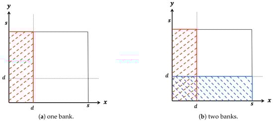
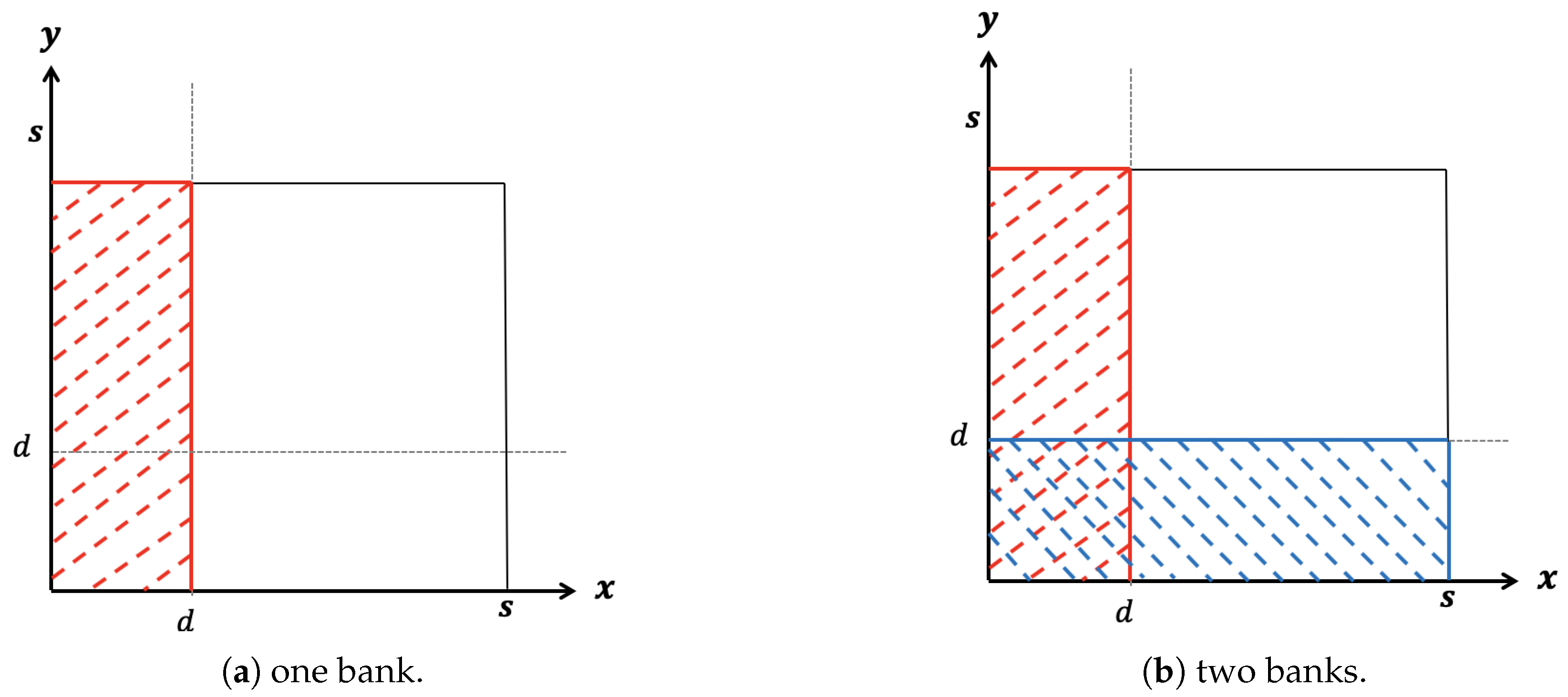
Now, without diversification, loan portfolio X would be the only asset of bank 1, and loan portfolio Y would be the only asset of bank 2. Hence, the gross return of each of the banks, if not liquidated, would simply be and respectively. Since a bank becomes insolvent and experiences a run whenever the gross return on the bank’s asset is insufficient to cover the bank run condition for bank 1 can be displayed as in Figure 1a; the dashed area represents the set of outcomes for bank 1’s failure. Bank 2’s case is added in Figure 1b, where the double dashed square represents the set of outcomes for a joint bank failure.
Figure 1.
Bank run outcomes in case of no diversification. (a) one bank (b) two banks.
However, once banks diversify by investing in both loan portfolios in various ways, the gross returns would change and, more importantly, the probabilities of individual and systemic bank failures would also change. This can be graphically verified by noting that a change in would change the border line, which divides bank run outcomes and no-bank run outcomes, which eventually would modify the probabilities of individual and join bank failures. The point is that a bank’s asset diversification affects not only the risk at the level of the individual bank but also the systemic risks of the entire banking sector. Let us now discuss each of the possible diversification strategies.
3. Diversification Strategies
To extend van Oordt (2014)’s model, we first present a general case of securitization, where the diversification strategies suggested in Wagner (2010) and van Oordt (2014) can be considered special cases. Suppose banks tranche the loan portfolio into securities with two different seniority levels and can sell these trenches to the other bank. On date 3, when the return on the bank asset is realized, the senior tranche is served first, up to the maximum set by the bank, whereas the junior tranche obtains the residual. Accordingly, the senior tranche on asset X has the payoff equal to , and the junior tranche has the payoff equal to . Similarly, each of the senior and junior tranches on asset Y has the payoff equal to and , respectively.
Bank i can choose to exchange fraction of the senior tranche and fraction of the junior tranche. The remaining portions and of the senior and junior tranches are kept on bank i’s balance sheet. Then, bank 1’s and bank 2’s respective returns on investment, if not liquidated, would be obtained as,
In this setup, different diversification strategies could emerge from the various combinations of and The simplest case would be no diversification, i.e., which would generate bank run outcomes described in Figure 1a,b. As mentioned before, in the rest of this section, we consider four diversification strategies: linear diversification without securitization, securitization with exchanging senior tranches only, securitization with exchanging junior tranches only, securitization with vertical distribution (which derives in linear diversification) and exchanging a portion of both tranches (mixed strategy).
3.1. Linear Diversification without Securitization
A bank can simply exchange a portion of its asset with the other bank without tranching. This type of diversification, which can be called linear diversification, is considered in Wagner (2010), and we recall it here for completeness. Since there is no tranching, we can have without the superscript S and denoting the fraction of bank i’s portfolio that is exchanged. Bank i’s return on investment, if not liquidated, is then
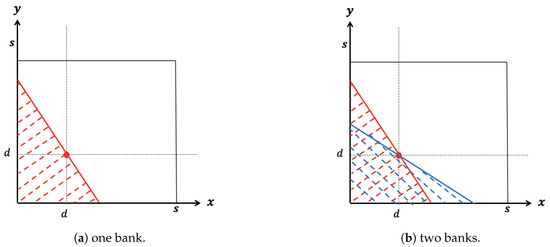
In this case, the bank run outcomes for bank 1 are represented by the dashed line in Figure 2a. The bank 2 failure outcomes are added in Figure 2b where the double dashed area represents the outcomes for a systemic crisis.
Figure 2.
Bank run outcomes in case of linear diversification. (a) one bank (b) two banks.
Wagner shows that linear diversification may reduce the probability of bank run on an individual bank when compared with no diversification, but it increases the probability of a systemic crisis. One can see this by observing Figure 2. For a formal proof, see Wagner (2010). This point illustrates the dark side of diversification4.
3.2. Securitization Retaining Junior Tranche (RJT)
In comparison to Wagner (2010)’s linear diversification, van Oordt (2014) introduces a non-linear diversification where banks securitize the loan portfolio into tranches and sell the senior tranche only. We call this strategy Retaining the Junior Tranche (RJT), and it corresponds to setting In this case, bank i’s return on investment in Equation (4), if not liquidated, becomes
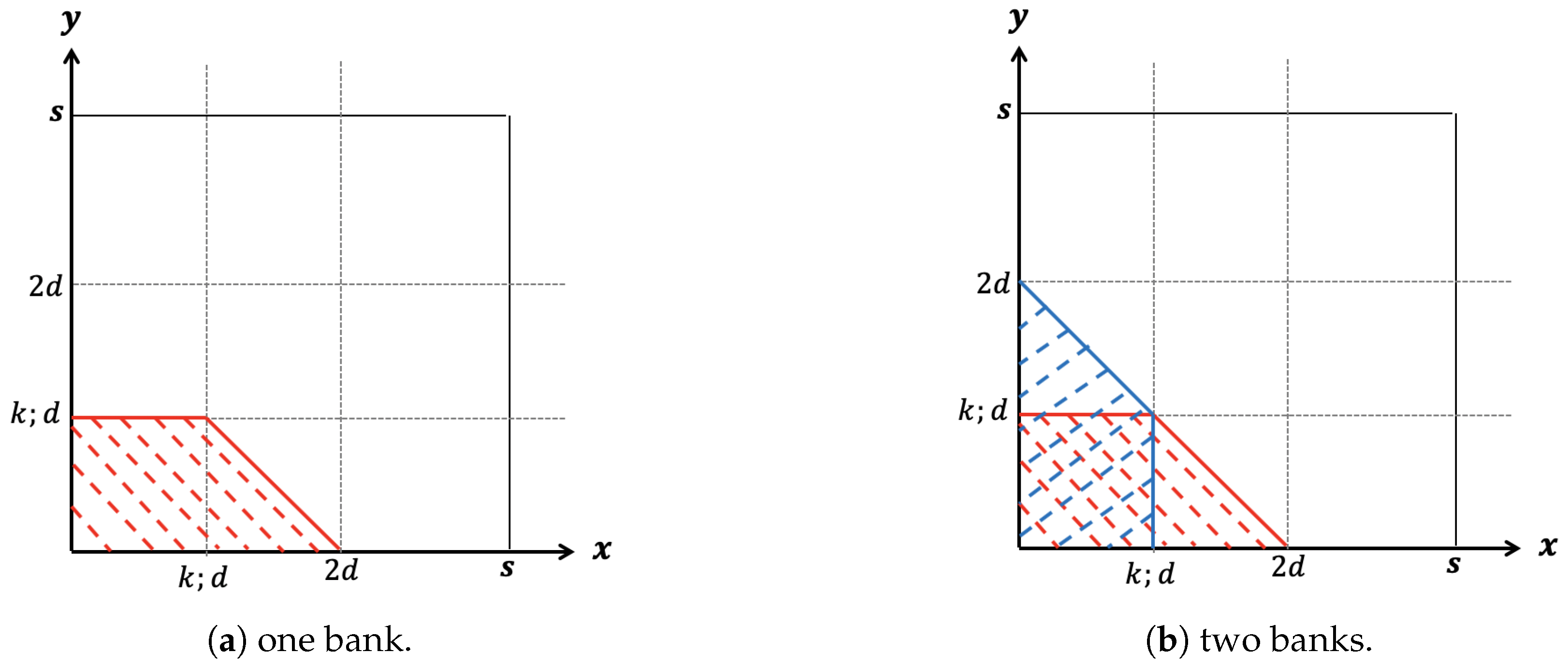
In this case, obtaining the bank run outcomes becomes complicated as it depends on the level of k vis-à-vis the level of van Oordt (2014) finds the different classes for the bank run outcomes and proves that for securitization that entails exchanging only the senior tranches, it holds that: (i) the probability of a systemic crisis cannot be decreased even with the RJT securitization; (ii) bank i’s optimal diversification strategy is the RJT securitization with and (individual optimality); and (iii) both banks adopting the strategy described in part (ii) is socially optimal (social optimality)5. If banks follow the optimal strategy suggested by van Oordt (2014), then the probabilities of failure would look as in Figure 3:
Figure 3.
Bank run outcomes for the optimal diversification strategy in case of securitization with keeping a senior tranche. (a) one bank (b) two banks.
3.3. Securitization with Vertical Distribution
If bank i sells the same portion of each tranche, i.e., , what we called vertical distribution, its investment return will be the same as that of the linear diversification strategy examined in Section 3.1. Hence, we obtain the following result,
Proposition 1.
Setting makes the securitization with vertical distribution effectively identical to the linear diversification strategy.
3.4. Securitization with Keeping Senior Tranche (RST)
When introducing the securitization with tranching into Wagner (2010)’s original model, van Oordt (2014) assumed that banks keep the junior tranche on their own balance sheet and exchange a fraction of the senior tranches. Although he states on a footnote that “It is irrelevant to the results whether we assume that banks exchange senior tranches and keep the junior tranche or vice versa”, we explore the validity of this assertion here. Our results are in agreement with van Oordt (2014), but we are interested in briefly exploring the implications of this result for the case of the non-linear effects in the financial system. As a further justification, van Oordt (2014) briefly mentioned asymmetric information between originators and buyers of securities as a potential mechanism that makes the strategy of exchanging senior tranches only an optimal structure. The information asymmetry may possibly arise when the buyers are outsiders such as institutional investors or nonbank firms without an understanding of the nature and composition of the securities they are purchasing. However, in the current model, the buyers of the securities are banks who themselves are securities originators and therefore may be better positioned than the outsiders when bidding for the tranches.
In this section, as mentioned before, we explicitly explore the possibility of the alternative strategy of keeping the senior tranche and selling the junior tranche only. We do this within the confines of the given model. The alternative securitization strategy we suggest corresponds to setting In this case, bank i’s return on investment is rewritten, if not liquidated, as
Or, alternatively,
Taking we find the no-bank run border for bank 1 to be:
Class 1: conditional on we have
Class 2: conditional on we have
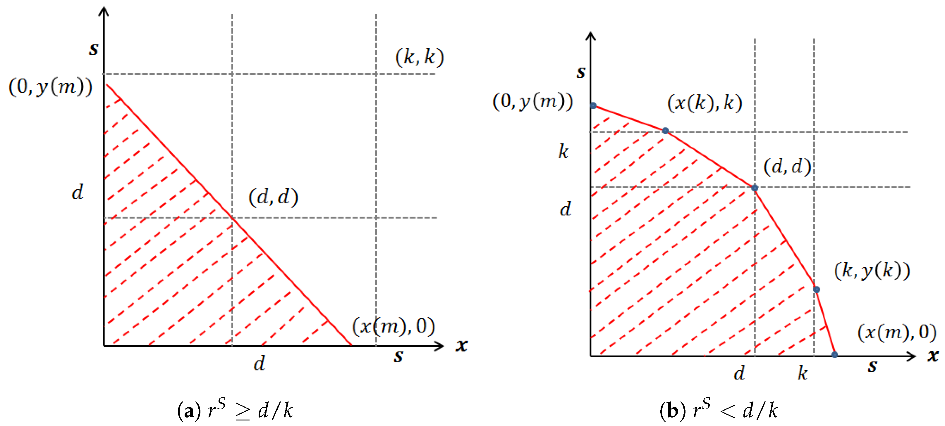
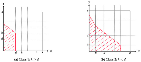
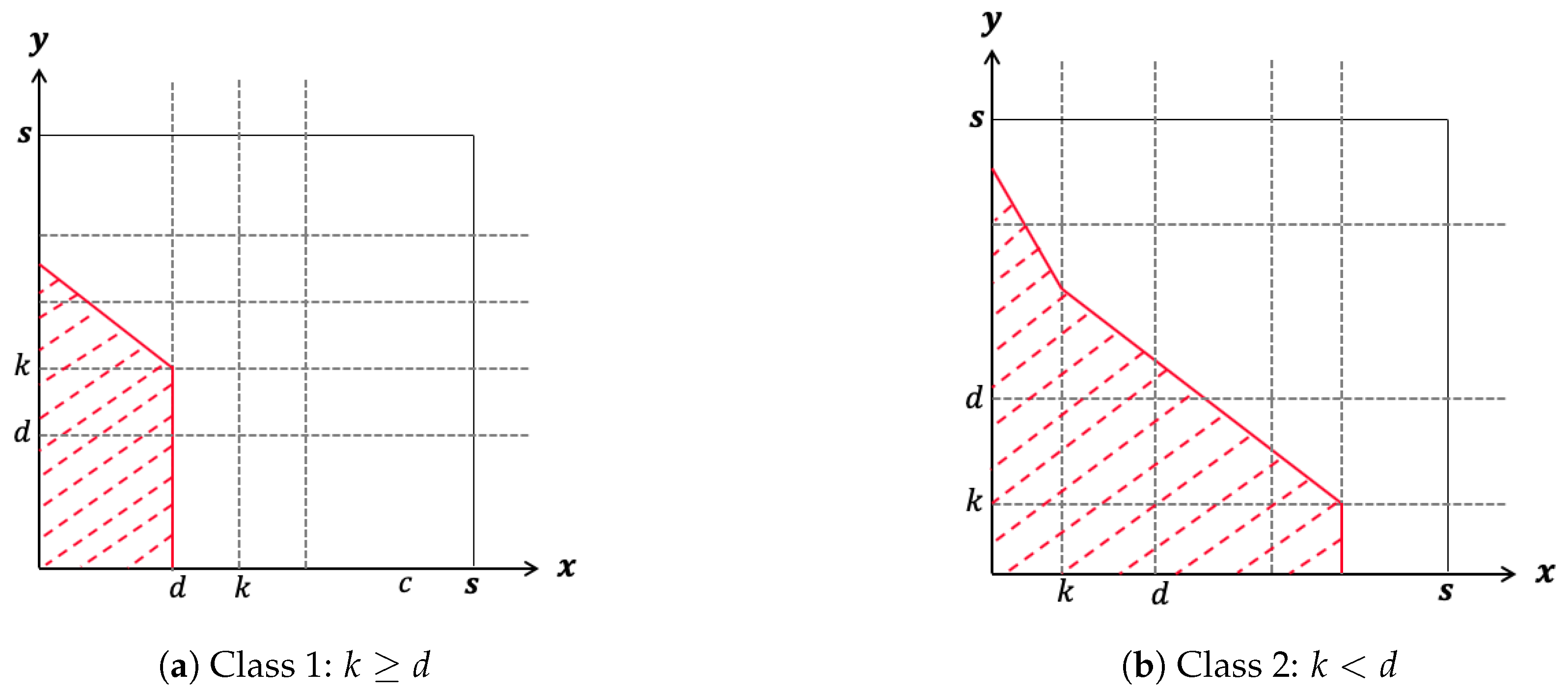
The set of bank run outcomes for a single bank within each of the two classes are displayed in the following Figure 46.
Figure 4.
No-bank run border for one bank under the strategy of exchanging only the junior tranche.
Results
Proposition 2.
If banks maintain the senior tranches only, as in (7), or if they keep both tranches in the same proportion (linear diversification), the probability of a joint failure cannot be decreased when compared to the no diversification case.
Although tranching does not decrease the probability of a joint failure, it does decrease the probability of a run on each individual bank. van Oordt (2014) shows this to be true for retaining the junior tranche only, and it will be shown in Proposition 3 to be true also for retaining the senior tranche in full.
Proposition 3.
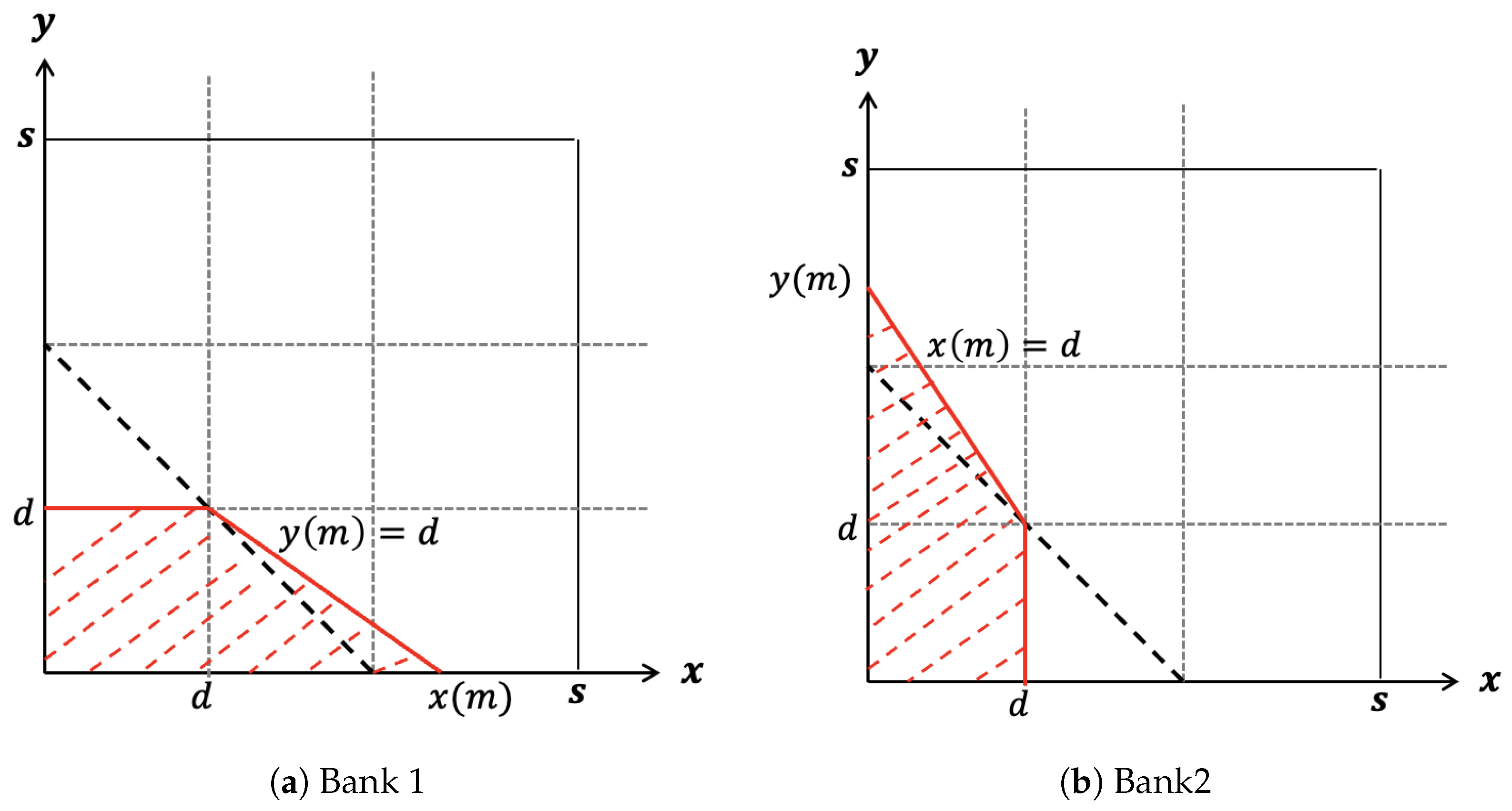
The probability of a run on bank i is minimized if and only if bank i sets the maximum payoff of the senior tranche equal to its level of deposits, i.e., and exchanges its junior tranche entirely ().
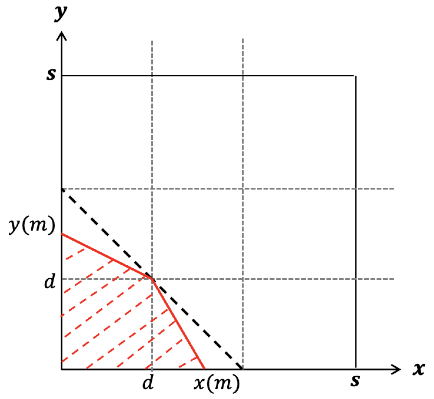
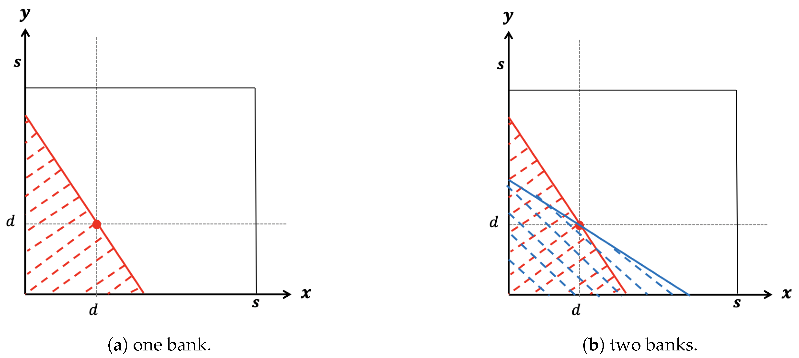
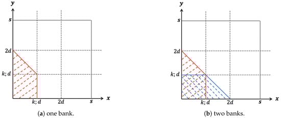
We illustrate the effectiveness of Proposition 3 in Figure 5a,b. Following (9), the no bank-run border for bank 1 under Proposition 3 is given by,
Figure 5.
Bank run outcomes for the optimal diversification strategy in case of securitization with keeping junior tranche.
The probability of bank 1 becoming insolvent under the strategy proposed is,
The expression in (11) is the outcome for the dashed area in Figure 5a. As it can be observed, the probability of a simultaneous bank run (Figure 5b) is not increased by trenching as defined in Proposition 3. As a consequence, minimizing the bank run probability also minimizes the expected costs of liquidation.
Proposition 4.
The optimal investment strategy that maximizes the total welfare in the economy, when exchanging only the junior tranche, is to set the maximum payoff of the senior tranche equal to its level of deposits, i.e., while exchanging its junior tranche entirely (). Since this strategy is the same when exchanging only the senior tranche, whether banks follow the optimal strategy from exchanging only the junior tranche or follow the optimal strategy from exchanging only the senior tranche, the total welfare of the economy is the same.
In other words, the total welfare of the economy does not change in situations where only the senior tranche, or only the junior tranche, is exchanged.
3.5. Securitization without Keeping Senior or Junior Tranche (Mixed)
In this section, we study the case in which none of the banks keeps the senior or junior tranche in full. As mentioned in Section 3, the returns for bank 1 and bank 2 if not liquidated are given by,
where in this particular case, and . Notice that zero and one are excluded from the set of options. These extreme cases are dealt with at the end. This case was not explored in van Oordt (2014). In Appendix B, we study the default region in the case (). From this geometric analysis, we gain intuition about how to move the parameters to minimize the size of the default probability. That analysis leads us to concentrate on case where the best hedging portfolios come up.
As the is a piecewise linear function, the default boundary is determined by the obvious break points The analysis in Appendix B is split into the cases and and this last case is further split into two cases according to whether or In addition to finding the breakpoints at the boundary, we determined how the points move when and vary. When the distribution of assets is uniform, the probability of default is the (normalized) area of the default region and it is not difficult to compute. Certainly, when the top and lateral breakpoints move to In this case, the position of the bank is given by:
Note that when or when that is along the diagonal and along the anti-diagonal in the parameter space, the hedges reduce to the linear diversification case. However, in the general case, there are two free parameters, and this allows us to move the default boundary to further decrease the default probability. It is in Appendix B.2.4 of Appendix B where we collect the computational details. Here, we mention that when and and the assets are uniformly distributed, the probability of default is given by (A26), that is, by:
Note that at , we obtain that the probability of individual failure is given by It is shown in Appendix B.2.5 of Appendix B that the point is a saddle point for given by (13). This drops out of the fact that the —Hessian matrix of has a positive and a negative eigenvalue. We denote by the negative eigenvalue and by its eigenvector. When a small enough is chosen, so that then
This explains why the bi-parametric hedge offers more possibilities for controlling default probability than the mono-parametric hedge. To sum up, we have the following result.
Theorem 1.
With the notations and under the assumptions introduced above, when each bank keeps the junior and the senior tranches, each bank may choose parameters (respectively, ) in in such a way that their individual default probabilities become (13) and satisfy (14); i.e., they are smaller than the individual default probability of the optimal linear hedge.
It is important to observe that the intersection of the individual default regions (i.e., the systemic risk) may have a larger probability of default than if no hedging is implemented. Hence, the dark side of diversification cannot be avoided when ) in . The dark side of diversification can only be avoided in the extreme cases: that is, when and or when and . The two-parametric dependence allows us two extreme cases, such that each bank can adopt one of them and lower the individual default probability without increasing the probability of joint default. This is discussed in Appendix B.2.6. The result is summed up in the following theorem. The result is stated without referring to any particular bank.
Theorem 2.
Suppose that the hedges of each bank are such that their returns are given by (12). For each bank, there are two extreme cases corresponding to or In the two cases, the default regions are as depicted in Figure A7a,b. In the first case, for , and in the second, for the probabilities of individual default satisfy
When the two banks adopt complementary hedges, their common region of default coincides with the no hedge region of default. Therefore, the dark side of diversification is avoided.
Controlling the Probability of Default
The results obtained above bring up the themes developed in Cadenas et al. (2021) or in Cadenas and Gzyl (2021). In the latter, we showed that one can control the individual and the systemic probability of default by considering short positions, whereas in the former, we discussed how and why the probability of default and loss level are complementary. If one assigns a probability of default, this determined what the default level is. The underlying reason is that risk involves two complementary aspects: frequency and severity.
The next result follows the approach in Cadenas et al. (2021). The idea is to fix the default rate and determine the default level so that the probability of default is at most the chosen probability. Let us denote that by p and note that if we equate the right hand side of (14) to p, we obtain
which allows us to choose an appropriate default level d if p is preassigned. When d is preassigned, a similar calculation allows us to choose the value of the parameter a as to lower the individual default probability to a value less than
4. Securitization and Confidence Shocks
Following van Oordt (2014), we analyze the results of retaining the senior tranche in the context of confidence shocks. van Oordt (2014) found that the benefits of securitization, when compared with linear diversification strategies, which consist of decreasing the probability of individual failures without increasing the probability of systemic risk, come at a cost. In other words, although structuring claims on loan portfolios using different seniority levels does not necessarily increase the probability of joint failures, it introduces non-linear effects in the financial system. Once banking institutions adopt the optimal strategy, small unanticipated shocks in confidence can increase considerably the risk of systemic failures. Given that banks do not have the knowledge to perfectly calibrate the payoffs of the tranches by setting the effects of confidence shocks become relevant to the analysis of trenching.
In this section, we compare the non-linear effects of different strategies: no diversification, linear diversification, retaining the junior tranche (RJT), retaining the senior tranche (RST), and exchanging a portion of both tranches (Mixed). We are particularly interested in comparing the RST, RJT and Mixed strategies, since this analysis has not been completed within the model. The shock in depositor’s confidence is modeled in the same way as in van Oordt (2014). The shock in depositors confidence occurs after the banks define their investment strategy at date 1. Depositors participate in a bank run if the return on the bank’s investments at date 2 is smaller than Therefore, if , a bank run may take place in a solvent bank.
We show here the expected liquidation costs for the four strategies mentioned and for specific levels of The expected default costs in the case of no tranching and no diversification are given by,
If banks follow the social optimal strategy with linear diversification as defined by Wagner (2010) where , the expected default costs are equal to,
If banks adopt the tranching strategy by retaining the junior tranche, the expected default costs are,
If banks adopt the tranching strategy by retaining the senior tranche, we find the expected default costs to be,
where , and
Finally, we explore what would happen if banks adopt the Mixed trenching strategy with , and we find the expected default costs to be,
Figure 6 shows the results of expected liquidation costs, joint probability failure and individual bank failure for different levels of 7. We found that when there is a sudden loss of confidence from depositors, the strategy based on retaining the senior tranche creates a considerable increase in the probability of both bank failings when compared with RJT. However, when retaining the senior tranche, the probability of individual failures becomes slightly better than the RJT strategy. Notice how the expected default costs are lower for both RST and RJT when compared with the no tranche and linear diversification strategy whenever As soon as this changes, that is after a confidence shock takes place, the expected default costs for both tranching strategies become considerably higher. One contribution of our simulation to the analysis of expected liquidation costs lies in showing that evaluating which strategy is considered “superior” depends on the magnitude of the shock. By observing the bottom graph in Figure 6, we see that RJT generates lower expected liquidation costs right after the shock takes place (i.e., for values of relatively close to 0.90) and that RST generates lower expected liquidation whenever It then follows, in the case of relatively “big” surprises in depositor’s confidence (we can measure the size of the surprise as the difference between and d), that the total welfare of the economy would be better managed by banks if they use the RST strategy over the RJT strategy.
Figure 6.
Diversification outcomes after a confidence shock.
Although, as it can be observed in Figure 6, the RST strategy leads to a considerably higher probability of systemic failure than the RJT strategy after the shock, RST does make the probability of individual failure smaller. In the case of securitization, as argued by Ordoñez (2018), the growth and collapse of securitization depend critically on the growth and collapse conditions that determine confidence in the system. Confidence, in turn, depends on reputation. Ordoñez (2018) defines reputation as the probability assigned by the market that a given firm is financially healthy. This generates incentives for banks to avoid bankruptcy whenever possible. It follows that a reasonable strategy for banks to avoid confidence shocks would be to avoid bankruptcy which, in this model, can be achieved by minimizing the probability of a banking institution failing. Under this assumption, banks will try to minimize the probability of a run by choosing the RST strategy. Such a decision would be even more clear if governments provide liquidity and support in the case of systemic crisis as the consequences of increasing the probability of a systemic failure would be mitigated; and the reputation problem of a bank failure will be carried by the entire banking system and not by one single institution.
The intuition of why the RST strategy seems to reduce the probability of individual failure comes from the fact that whenever the returns of the bank’s asset (say asset X) are very low, the return on the senior tranche that was exchanged in the case of the RJT strategy is bounded by Hence, even if the return of asset Y is quite high, the bank can only achieve in this case a return of In contrast, the return on the junior tranche that was exchanged with the other bank in the case of the RST strategy is not bounded by a minimum value, and it may leave open the possibility of no failure whenever y is sufficiently high.
Securitization strategies that exchange both tranches illustrate, along with vertical distribution, the dark side of diversification. It may be worth emphasizing the point that the mixed strategy can reduce the probability of individual failure when compared with the linear diversification strategy, but it does so at the cost of considerably increasing the probability of joint failure and the expected liquidation costs of banks in the case of confidence shocks. The analysis of confidence shocks reinforces the point that, from the perspective of managing risk, banks are better off by only exchanging one of the tranches rather than exchanging two.
5. Discussion
Banks can construct portfolios that are identical to linear diversification by using securitization strategies. That is to say, linear diversification is actually a subcase of securitization strategies designed around senior and junior tranches. As it has been argued by Wagner (2010) and van Oordt (2014), with linear strategies comes the problem of the dark side of diversification. In other words, linear diversification strategies have the problem that as banks reduce the probability of individual failure, then the failure of the entire banking system becomes more likely. Similar points have been illustrated in other theoretical and empirical studies (Acharya 2009; Allen et al. 2012; Allen and Carletti 2006; Ibragimov et al. 2011; Wagner 2010; Yang et al. 2020).
One way to avoid the dark side of diversification, as discussed by van Oordt (2014), is to keep the junior tranche and exchange the senior tranche (RJT). However, what about all other theoretical possibilities that are available within the securitization scheme? The present study provides an answer to this question by generalizing van Oordt’s (2014) model for long positions and studying the problem of diversification and systemic risk. In particular, it shows that the dark side of diversification can be also avoided by exchanging the entire junior tranche and keeping in full the senior (RST). We also showed that, in this case, there is no difference from the point of view of the welfare of the entire system. However, the strategy of keeping the senior tranche and exchanging the junior leads to worst outcomes, from the point of view of systemic risk, when confidence shocks are being considered. From the point of view of expected liquidation costs, we did not find major differences between RST and RJT. Regulators could potentially contribute to reduce confidence shocks by providing liquidity support in the case of a systemic failure.
When it comes to the use of a mixed strategy (i.e., exchanging a portion of both tranches), it is possible to reduce the probability of individual failure when compared to linear diversification. Nevertheless, such a strategy does not avoid the dark side of diversification. From the point of view of confidence shocks, mixed strategies that are close or equal to exchanging portions of both tranches in the same proportion result in worst outcomes than all other possible strategies. Hence, mixed strategies are problematic and should be avoided by banks. Accordingly, the benefits of securitization can only be felt at the extremes. By exchanging one of the tranches in its entirety, banks can reduce the risk of individual failure without increasing systemic risk, reduce social costs, and minimize idiosyncratic and systemic risks in the case of confidence shocks when compared with other securitization strategies.
The theoretical suggestion that banks are better off by adopting securitization strategies that exchange only one tranche seems to be in accordance with the idea that transparency is central in avoiding systemic crisis. After all, exchanging only one portion makes the banks portfolios less complicated, easier to track and, consequently, more transparent. As it has been argued by Klein et al. (2021), poor transparency of asset-backed securities exacerbated the latest subprime lending crisis. Our theoretical results do not contradict the importance of transparency in the banking system. In fact, it reinforces the relevance of this idea for banking institutions and regulators. In addition, our theoretical results are in line with the empirical work of Deku et al. (2019) in the sense that securitization is not a destabilizing tool per se. The destabilizing forces that are introduced by securitization depend on how the instruments are designed and used. Regulation, in turn, can eliminate undesired outcomes by, for example, enforcing the design of securitization instruments that don’t allow the exchange of both tranches.
We believe that both theoretical and empirical work are necessary for a better understanding of securitization, diversification and the fragility of the banking system. Theory can help illuminate the extent and detail of empirical studies, and empirical studies can guide the questions posed in theoretical work. To the best of our knowledge, most of the recent research in this area (during the past four years) has been predominantly empirical in its approach. Part of our contribution is based on the idea that theory may provide further sources for understanding the use of securitization tools and to better inform policy makers and regulators.
One direction that remains to be explored is to investigate if the conclusions of the theoretical framework presented in the present study hold when more banks and assets are considered.
Author Contributions
Conceptualization, P.C.; methodology, P.C. and H.G.; formal analysis, P.C. and H.G.; investigation, P.C.; resources, P.C.; writing—original draft preparation, P.C.; writing—review and editing, P.C. All authors have read and agreed to the published version of the manuscript.
Funding
This research received no external funding.
Institutional Review Board Statement
Not applicable.
Informed Consent Statement
Not applicable.
Data Availability Statement
Not applicable.
Acknowledgments
We would like to thank Hyun Woong Park for his valuable contributions in helping setting up the first part of the exercise of generalizing Oordt’s model. We are also grateful for some of his comments and suggestions for an early draft of this paper. The usual disclaimer applies.
Conflicts of Interest
The authors declare no conflict of interest.
Appendix A. Proofs
Appendix A.1. Derivation of the No Bank Run Border (x)
The set of possible returns for bank i to be solvent is derived from solving Following (7), bank 1’s returns are given by,
The solution to the no bank run border can be found by the union of the following subsets:
For keeping the senior tranche entirely, we separate the solution into two cases as shown in (8) and (9): case 1 where and case 2 where
Case 1: Subset A is empty (i.e., the bank always fails) for . If and ; then, the condition is always fulfilled and the bank never fails. Subset B needs to satisfy for and . Within subset B if , then the condition is always satisfied since and Subset C is always true because implies that (i.e., since and ). Finally, the condition in subset D is always satisfied because , which is an expression that comes from rewriting The union of all subsets can be written as Equation (8), which provides the minimum return y that is necessary for bank 1 to be solvent given the returns of whenever
Case 2: Subset A is empty given that (). Subset B needs to satisfy the condition for as Subset C is empty when since the condition would fail in this case. Notice that (because ) and (since ), given If , then the condition of subset C is true and there is no bank run. The condition in subset D for also has two parts. For , the condition of D needs to be satisfied. If, on the other hand, , then the condition is true for the entire interval. To see this, notice that If we substitute the lowest possible value that x can take, namely , we would obtain which is true since If holds for , then it must hold also for ; since Hence, for this last interval, the condition in D is always satisfied, and there is no bank failure. The unions of these subsets result in Equation (9).
Appendix A.2. Proof of Proposition 1
The no tranching or no diversification case is given by setting For bank 1, we know that its returns are given by,
For ; Therefore, in this case, the return of each bank will depend solely on the asset owned. The no bank run border is given by Equations (8) and (9). Making and if , then the banks fail in both case 1 and case 2. For case 1, we would end up with the condition that (after substituting r by zero), which cannot be true for For case 2, first observe that the expression when If , then we need to consider the first of the three expressions. In the first case, when substituting r by zero, we would have the same expression as in case 1, which is false for If , we would then also have that which fails for It follows that for the case of no trenching–no diversification, a systemic failure occurs when and
When allowing for trenching (RST) and linear diversification (via vertical distribution: ), we have the following results: For RST, if and then Equation (8) cannot be satisfied since , which is false for and If then we find is also false for and When , then fails for Hence, for RST, both banks fail at the same time—due to symmetry—whenever for any and any .
For the case of linear diversification or vertical distribution, as shown by Wagner (2010) and van Oordt (2014), both banks fail whenever and which holds in our case for any and as long as Therefore, irrespective of tranching or linear diversification, a systemic failure takes place when both and .
Appendix A.3. Proof of Proposition 2
We follow the same general strategy, and notation, used by van Oordt (2014). That is to say, we prove this proposition by showing that for any and any , except and The probability of a bank run for each strategy can be obtained by taking the surface integral of over the area below the no bank run border.
where The strategy for proving is to show that either or Comparing (A2), (A4) and (A6), it follows that it is sufficient to demonstrate either
or
Figure A1.
.
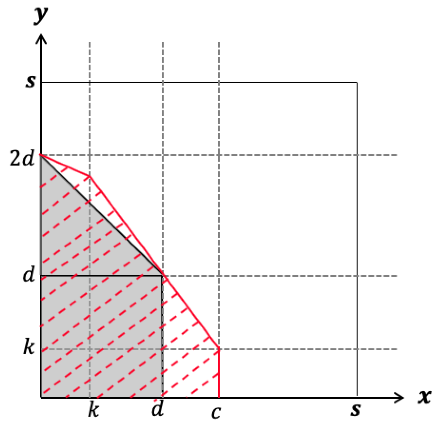
Figure A2.
.
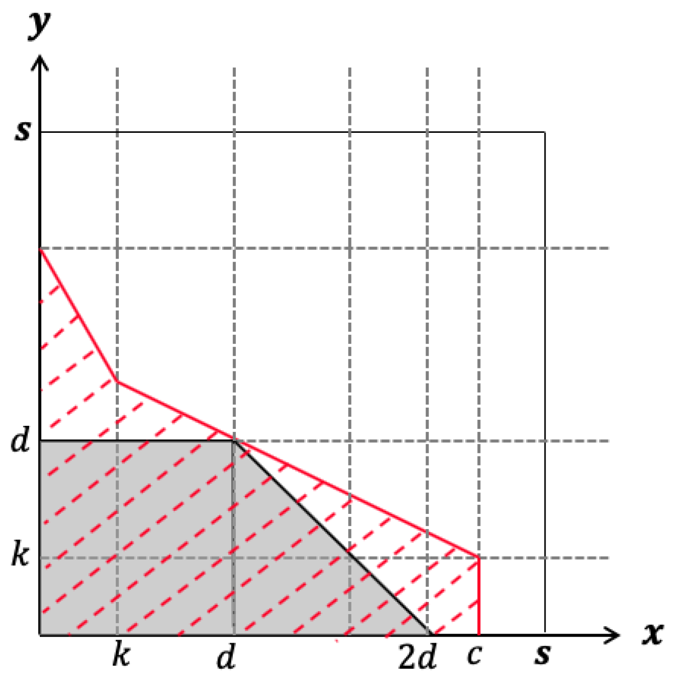
Figure A3.
.
We need to show this for any and , except and Starting with case 1 (), the no bank run border is given by Equation (8). For , we must show that We can rewrite this expression as,
Since then the condition will always be true for any . For , there is no probability of failure, so it follows that
We now consider Case 2 () where the no bank run border is given by Equation (9). First, we examine the case for (Figure A1). For , there are two no bank run borders: one for and another for . We start with , where we need to show that Equation (A11) is true for but when We begin by noticing that and and that both are linear functions. Hence, the left-hand expression of Equation (A11) is bounded above by , in which case the right-hand expression is equal to d satisfying the condition. Checking the other extreme, we notice that the right-hand expression of (A11) is bounded below by zero, in which case the right-hand side is , satisfying the condition as well. It follows that for and
For the case when and , where Figure A2 provides an illustration, because of symmetry, we obtain,
For we need to consider two parts. First, let us consider what happens when . From Equation (9), we need to show that This is equivalent to , which is true for . Second, we consider the case when in which case the bank cannot fail and, thus, there is no probability of failure (i.e., ).
The last case, when and , is illustrated in Figure A3. For the first part of this case, we start by observing, in similar fashion as van Oordt (2014), that:
where m is the value of x for which in the interval That results in . The inequality in (A13) holds because and equality holds because of the symmetry of . We also know that,
where,
As a consequence, we need to demonstrate that for both and In this manner, we will prove that For , we need to demonstrate that This is the same as . This is precisely the value of m, which is the upper bound of this interval. It follows that this condition is true for any . For we need to show that This expression can be also be written as . This is true for any value of x in the interval and for any . Hence, .
Appendix A.4. Proof of Proposition 3
The returns for bank 1 and 2 that are obtained from retaining the senior tranche (RST) strategy () are defined as,
The returns for bank 1 and 2 that are obtained from retaining the junior tranche (RJT) strategy () are defined as,
Since the returns on x and y are independent and identically distributed, and by comparing (A16) with (A19), and (A17) with (A18), it follows that:
and
The expected value for bank i is written as,
Since the expected values are the same in both strategies (RST and RJT), it follows that maximizing the welfare is equivalent to minimizing the probability of individual failure. Since, as it was shown in the previous proposition, minimizing the risk entails setting and for both strategies, it then follows that the expected value of each bank is the same regardless of which of the two strategies is adopted. In addition, given that the total welfare of the economy is given by,
We see that the total welfare of the economy is the same if banks follow the optimal strategy for both cases (i.e., RST and RJT).
Appendix B. Details for Section 3.5
The return for bank 1 and 2, if not liquidated, are given by Equation (12),
Here, we will analyze the default region of only. Given that the analysis of the position of the other bank is exactly similar, we will skip it and, to simplify our notation, we will drop the subscript from and denote it by r instead. There are a few cases and sub-cases to consider. The two cases correspond to and To begin, note that is piecewise linear in x or and there are natural breakpoints at the points in the -plane. These are the intercepts of the default boundary with the lines and In addition, the point is on the default boundary. Below, we determine the lines and examine how the intercepts move when the parameters vary. Note that the breakpoints are the extremal points of a convex region which describes the default region.
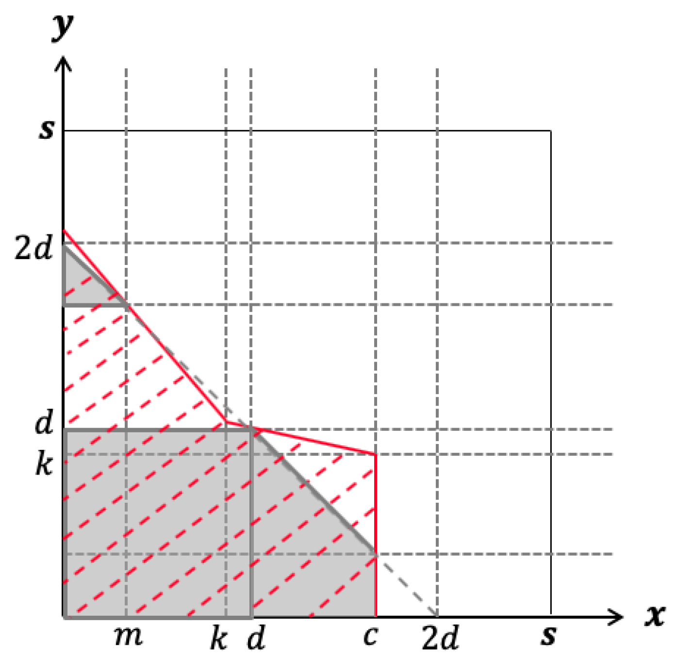
Appendix B.1. Case k ≤ d
The intercept of the with the vertical axis is with Notice that Of course, the point is in the default region.
The point where the vertical line intersects is It is easily verified that The boundary line determined by these points and consists of the lines
To determine the intercept of the line with the x-axis, solve to obtain It follows that Let us now consider the intercept of the line with Solving , we obtain The rest of the boundary is given by the lines joining to and to These lines are given by
Observe that the two central segments combine into one single line. The default region in this case is displayed in Figure A4.
Figure A4.
Case .
Motion of the Breakpoints for the Case k < d
Let us examine how the breakpoints in Figure A4 move when the parameters and change. Let us examine the signs of the derivatives of with respect to these parameters.
That is, the breakpoints on the “upper lid” of the default region move down along the line as the parameters increase, but the “right lid” moves out. This suggests that could be an optimal point.
Appendix B.2. Case d < k
This time, we have to consider two cases depending on whether or
Appendix B.2.1. Case rS ≥ d/k
We have to examine two cases for the intercept with . Either or In the first case, we have , which is compatible with the condition In the second case, we obtain The condition implies that we must have , which contradicts our assumption.
In the first case, the line
is the boundary line connecting to To find what happens to the right of , we must consider two cases for the intercept and the line Either or In the first case, we obtain and the condition implies In this case, the line from to is the default boundary. It is given by
The default boundary in this case is displayed in Figure A5a below. Note that since the slope of the two segments is the same, the line is similar to that of Figure 1a.
Appendix B.2.2. Case rS < d/k
In this case, it is easy to rule out the possibility of as incompatible with The alternative is Then, in this case, there is a break point at with The boundary between and consists of two lines given by
To determine the default boundary beyond , we also consider two possibilities for the intercept of and the -axis. Either or The first case leads to with the condition The other case yields In this case, there is a break point at with
Notice that again, the slopes of the lines and are equal and the common line passes through This case is similar to the first case except that the roles of d and k are interchanged. The default region is displayed in Figure A5b.
Figure A5.
The default region when .
Appendix B.2.3. Motion of the Break Points for the Case k > d and rS ≤ d/k
This time, we examine how the break points in Figure A5b move when the parameters and change. Again, we compute the derivatives of with respect to these parameters.
Note that as increases, the point moves to the right along the line that joins to Similarly, slides up along the line from to when increases.
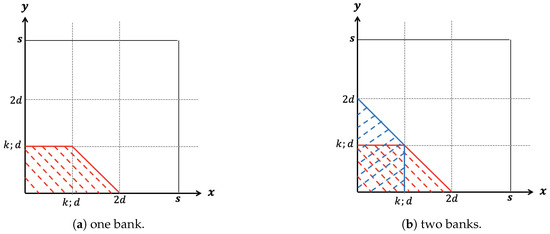
Appendix B.2.4. Analysis of the Effect of the Tranching When k = d
From the above calculations, it is clear that to decrease the individual probabilities of default, we must consider the case We restrict our analysis to the case When , the middle break point disappears, and the default boundary consists of two straight lines joining the points and to Since this time (dropping the unnecessary subscript):
As the cases or reduce to the case studied by Wagner, we shall keep them different and examine which combination of values is such that the default region is below the line For that, we are going to examine the values such that or The computations are not difficult, and the result is contained in the following result.
Theorem A1.
With the notations introduced above, the intercepts and of the broken line with the coordinate axes are given by
The constraints upon and for and are given by:
The extreme cases will be discussed separately below. Note also that when , the points and move in opposite directions along their axes when or change:
A little computation shows that the probability of default in this case is
Observe that for values of close to 0 or to the expression for P becomes larger than Therefore, we suppose that is close to in a range that depends on and
Appendix B.2.5. Analysis of the Probability of Default (A26)
We shall now verify that is a saddle point for the probability given by (A26). For short, let us write for a while.
is a root of the system. The Hessian matrix at can be computed by differentiating the equations displayed above with respect to and/or and evaluating at It is given by
Its determinant is negative, which suggests a saddle point. The eigenvalues of are
The two un-normalized eigenvectors are:
They are clearly orthogonal. Let us denote their normalized versions by and Notice now that if we set
with a small enough, then expanding up to second order in a, we obtain
Similarly, substituting and obtained from (A27) into Equation (A23) yields the intersection points of the default domain with the -axes. We round up the above remarks into:
Theorem A2.
With the notations introduced above, let be small enough so that Then, the probability of default of the hedge
is given by (A28); that is, a can be chosen so that
In Figure A6, we show the default region for this case relative to Wagner’s optimal case.
Figure A6.
Default region for .
Appendix B.2.6. Extreme Cases
Case 1:
This case reduces to Wagner’s (2010) case
In this case, we have two subcases for the intersects with the axes. If , we have and and the opposite happening when This was analyzed from a different point of view in Cadenas and Gzyl (2021).
Case 2:
Here, we obtain an extension of Wagner’s and Oordt’s hedges, which is given by
We put for brevity. This is a rather curious case, as the probability of default of the bank is independent of the hedge, and it is easy to see from (A26) that it equals
independently of the value of It can be verified that in this case, the default boundary coincides with that of the previous case when
Case 3:
To set requires that , which in turn implies that With an eye on the second equation in (A25), we see that if we make as small as possible, will be as close as possible to without violating the requirement for Not only that, this is nice, because for being small, we insure that as well.
In this case, the probability of default (A26) reduces to
In this case, this is smaller than for and tends to
Case 4:
This time, it is required that and since necessarily for the condition can not be satisfied. In addition, when , then for and for As above, when is close to then , and this is nice because
Now, the probability of default is
We have for
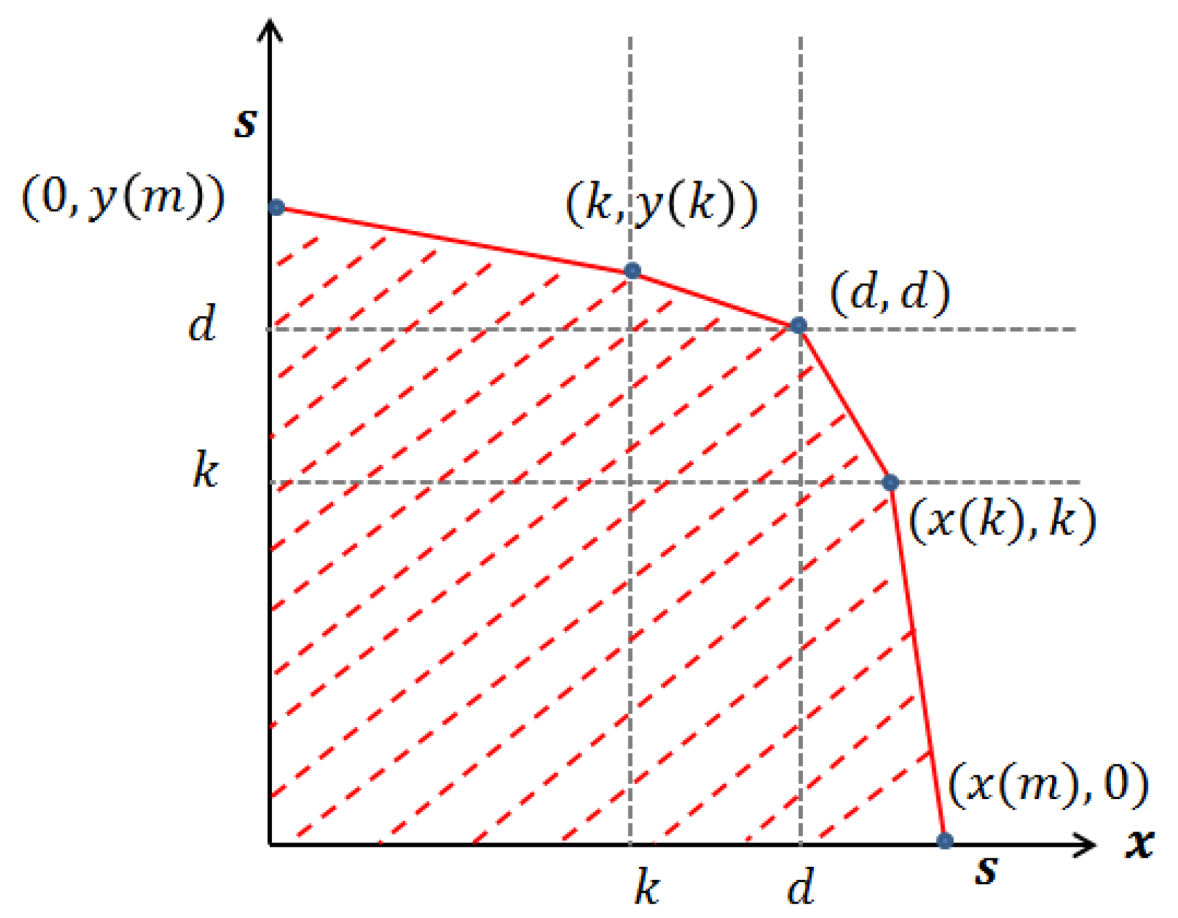
We close this section by pointing out that in Figure A7a,b, we display the case when the two banks adopt complementary hedges. This time, the systemic probability of default is not increased, while the individual default probabilities can be lowered. Apart from the possibility of using short positions analyzed in Cadenas and Gzyl (2021), this seems to be the only possibility of lowering the individual default probabilities without increasing the probability of systemic default.
Figure A7.
Complementary hedges for the two banks.
Notes
| 1 | Under the condition that is a uniform distribution function, expression (1) implies . |
| 2 | It would be more precise to have the total liability including both principal and interest as the minimum value of gross asset return needed to avoid a failure. Having as the condition of a bank run—following Wagner (2010) and van Oordt (2014)—is to assume that the cost of borrowing is zero. However, explicitly incorporating a positive deposit interest rate does not change the result qualitatively as long as the interest rate is held constant. |
| 3 | Alternatively, we can examine the bank’s decision from the shareholders’ perspective and thus consider the maximization of equity value. |
| 4 | We studied a variation of this using short positions in Cadenas and Gzyl (2021). |
| 5 | For a formal proof, see van Oordt (2014). |
| 6 | which means that any return of y would be sufficient to avoid a run on bank i (given the support of the density function in ). |
| 7 | The parameter choices in Figure 6 are , , and . |
References
- Abdelsalam, Omneya, Marwa Elnahass, Habib Ahmed, and Julian Williams. 2022. Asset securitization and bank stability: Evidence from different banking systems. Global Finance Journal 51: 100551. [Google Scholar] [CrossRef]
- Acharya, Viral V. 2009. A theory of systemic risk and design of prudential bank regulation. Journal of Financial Stability 5: 224–55. [Google Scholar] [CrossRef]
- Allen, Franklin, Ana Babus, and Elena Carletti. 2012. Asset commonality, debt maturity and systemic risk. Journal of Financial Economics 104: 519–34. [Google Scholar] [CrossRef]
- Allen, Franklin, and Elena Carletti. 2006. Credit risk transfer and contagion. Journal of Monetary Economics 53: 89–111. [Google Scholar] [CrossRef]
- Altunbas, Yener, David Marques-Ibanez, Michiel van Leuvensteijn, and Tianshu Zhao. 2022. Market power and bank systemic risk: Role of securitization and bank capital. Journal of Banking Finance 86: 106451. [Google Scholar] [CrossRef]
- Bégin, Jean-François, Mathieu Boudreault, Delia Alexandra Doljanu, and Geneviève Gauthier. 2019. Credit and Systemic Risks in the Financial Services Sector: Evidence from the 2008 Global Crisis. The Journal of Risk and Insurance 5: 263–96. [Google Scholar] [CrossRef]
- Ben Salah, N., and Hassouna Fedhila. 2012. Effects of Securitization on Credit Risk and Banking Stability: Empirical Evidence from American Commercial Banks. International Journal of Economics and Finance 4: 194–207. [Google Scholar]
- Cadenas, Pedro, and Henryk Gzyl. 2021. Diversification Can Control Probability of Default or Risk, but Not Both. Journal of Risk and Financial Management 14: 73. [Google Scholar] [CrossRef]
- Cadenas, Pedro E., Henryk Gzyl, and Hyun Woong Park. 2021. How dark is the dark side of diversification? The Journal of Risk Finance 22: 44–55. [Google Scholar] [CrossRef]
- De Jonghe, Olivier. 2010. Back to the basics in banking? A micro-analysis of banking system stability. Journal of Financial Intermediation 19: 387–417. [Google Scholar] [CrossRef]
- Deku, Solomon Y., Alper Kara, and Yifan Zhou. 2019. Securitization, bank behavior and financial stability: A systematic review of the recent empirical literature. International Review of Financial Analysis 46: 245–54. [Google Scholar] [CrossRef]
- Ibragimov, Rustam, Dwight Jaffee, and Johan Walden. 2011. Diversification disasters. The Journal of Financial Economics 99: 333–48. [Google Scholar] [CrossRef]
- Ivanov, Katerina, and Julia Jiang. 2020. Does securitization escalate bank’s sensitivity to systemic risk? The Journal of Risk Finance 21: 1–22. [Google Scholar] [CrossRef]
- Klein, Philipp, Carina Mössinger, and Andreas Pfingsten. 2021. Transparency as a remedy for agency problems in securitization? The case of ECB’s loan-level reporting initiative. Journal of Financial Intermediation 46: 214–31. [Google Scholar] [CrossRef]
- Ordoñez, Guillermo. 2018. Confidence banking and strategic default. Journal of Monetary Economics 100: 101–13. [Google Scholar] [CrossRef]
- Slijkerman, Jan Frederik, Dirk Schoenmaker, and Casper G. de Vries. 2013. Systemic risk and diversification across European banks and insurers. Journal of Banking and Finance 37: 773–85. [Google Scholar] [CrossRef]
- van Oordt, Maarten. 2014. Securitization and the dark side of diversification. Journal of Financial Intermediation 23: 214–31. [Google Scholar] [CrossRef]
- Wagner, Wolf. 2010. Diversification at financial institutions and systemic crises. Journal of Financial Intermediation 19: 375–86. [Google Scholar] [CrossRef]
- Yang, Hsin-Feng, Chih-Liang Liu, and Ray Yeutien Chou. 2020. Bank diversification and systemic risk. The Quarterly Review of Economics and Finance 77: 311–26. [Google Scholar] [CrossRef]
Publisher’s Note: MDPI stays neutral with regard to jurisdictional claims in published maps and institutional affiliations. |
© 2022 by the authors. Licensee MDPI, Basel, Switzerland. This article is an open access article distributed under the terms and conditions of the Creative Commons Attribution (CC BY) license (https://creativecommons.org/licenses/by/4.0/).