
Are Banks Still a Risk Source for Stock Market? Some Empirical Evidences


Abstract
:1. Introduction and Literature Review
2. Econometric Model
2.1. VECM Model
- is the sector price index at time t;
- is the market benchmark price index at time t;
- is the i-th bank stock price at time t.
- and are, respectively, the first differences for the Sector Relative Return to Benchmark and the i-th Bank Relative Return to Sector series;
- and are, respectively, the constant terms of the Equations (3) and (4);
- and are, respectively, the delayed first differences for Sector Relative Return to Benchmark and for the i-th Bank Relative Return to Sector series;
- is the number of lags;
- is the Error Correction Term (ECT). It is defined as , where is the cointegrating coefficient and is the intercept of the cointegrating term. The ECT measures the deviations between the Sector Relative Return to Benchmark and the i-th Bank Relative Return to Sector at time with respect to the theoretical long-period equilibrium;
- and are the adjustment coefficients, which describe the adjustment speed to the long period equilibrium, meaning, the strength of correction from the series deviations back to the long-run relationship;
- and are, respectively, the error terms of the Equations (3) and (4).
- is statistically significant and negative. This means that i-th Bank Relative Return to Sector series adjusts more rapidly than the Sector Relative Return to Benchmark. This means that the latter is trying to restore the long-run equilibrium;
- is statistically significant and positive. This means that the Sector Relative Return to Benchmark series adjusts more rapidly than the i-th Bank Relative Return to Sector. This means that the latter is trying to restore the long-run equilibrium;
- is statistically significant and negative and is statistically significant and positive. In this case, both variables contribute to the adjustment process towards the long-run equilibrium. Following Gonzalo and Granger (1995), in order to evaluate the effective contribution of each variable in the adjustment process, in terms of the Market Share (MS)6 concept, we can distinguish three subcases:
- If , then the Sector Relative Return to Benchmark variable is the leading (causing) variable and the i-th Bank Relative Return to Sector variable is the lagging (effected) variable;
- If , then the i-th Bank Relative Return to Sector variable is the leading (causing) variable and the Sector Relative Return to Benchmark variable is the lagging (affected) variable;
- If , then both variables contribute in the same way;
- Only one of the adjustment coefficients is statistically significant and it presents the correct sign. Then, only the significant variable contributes to the adjustment process toward the equilibrium.
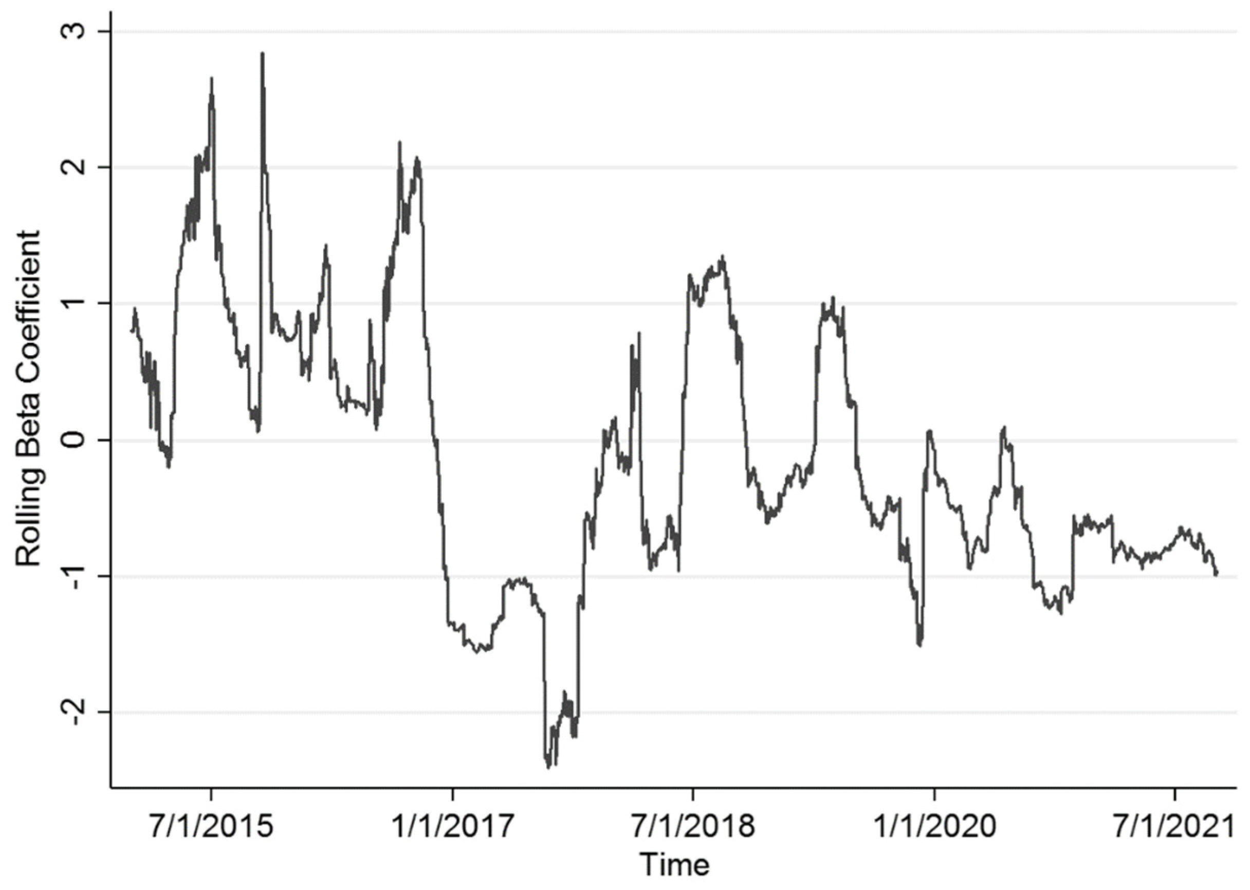
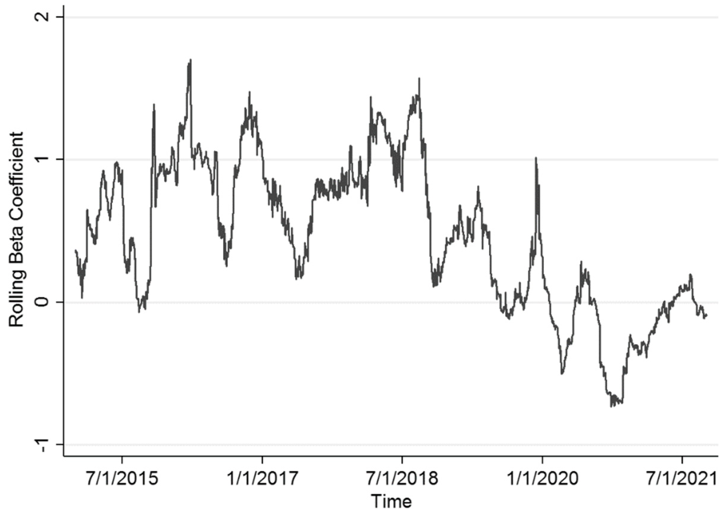
2.2. Rolling Regression
- is the constant at time t;
- is the beta coefficient of regression at time t;
- is the error term at time t.
3. Data Description
3.1. Euro Area General Framework
3.2. Data
- at time t;
- for the i-th bank in the selected sample at time t;
- at time t.
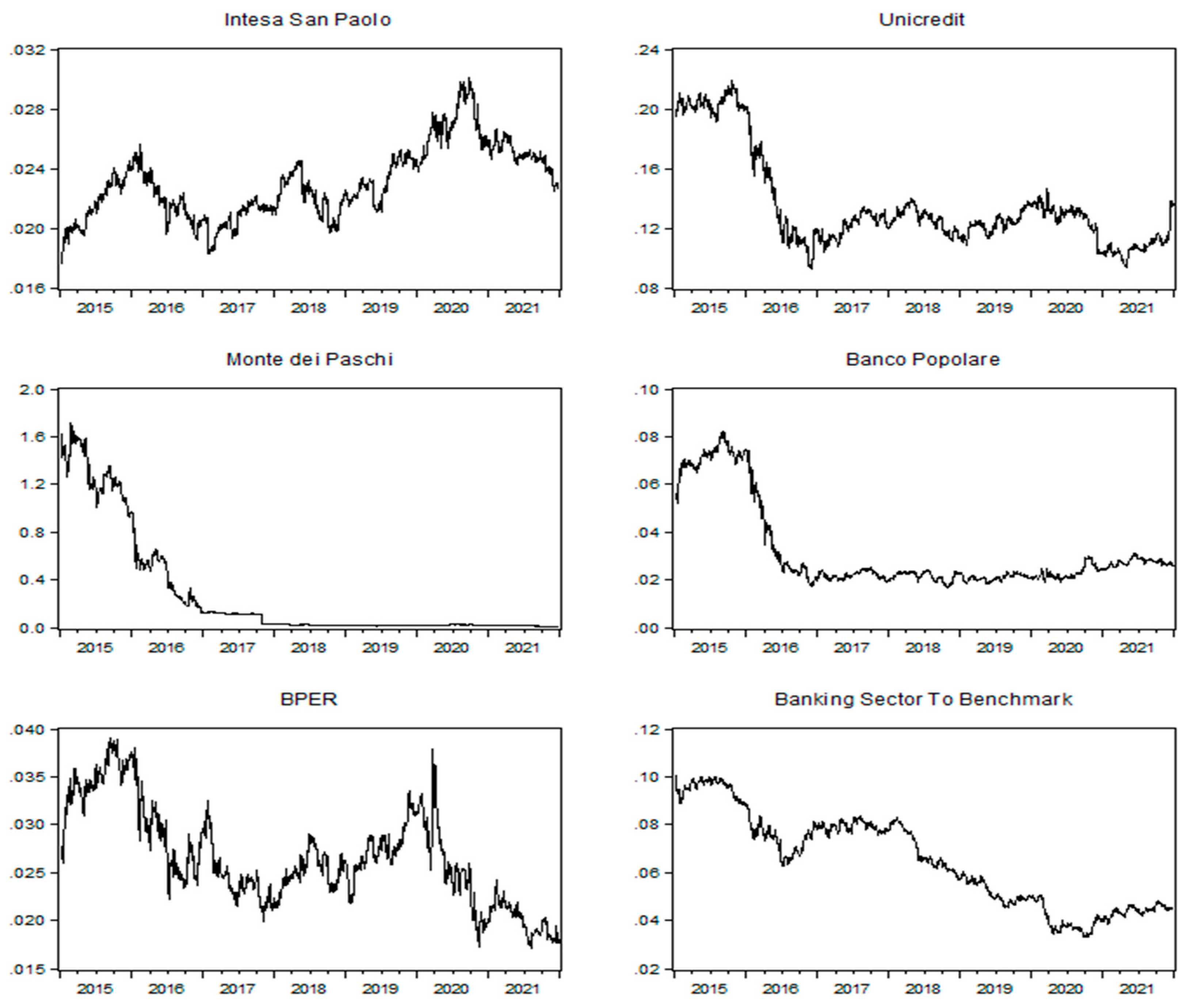
- Intesa San Paolo;
- Unicredit;
- Banca Monte dei Paschi di Siena;
- Banco BPM;
- BPER Banca.
4. Empirical Findings
5. Conclusions and Discussion
Author Contributions
Funding
Informed Consent Statement
Conflicts of Interest
| 1 | Source: Borsa Italiana, www.borsaitaliana.it (accessed on 19 March 2022). |
| 2 | Source: World Bank, https://data.worldbank.org (accessed on 19 March 2022). |
| 3 | A moving window regression is performed considering a fixed-length subset (window) of a time series, and by shifting the window’s starting point of a specified value each time. |
| 4 | “Shock” is an unexpected changing event that can have positive or negative effects on one or more correlated variables. |
| 5 | Theoretically, we can not exclude that results in a positive value, and that can have a negative value, but in these cases the process would result in the shock amplification, instead of the adjustment toward the long-run equilibrium. |
| 6 | The formula suggested by Gonzalo and Granger (1995) is the following: . |
| 7 | ADF test proves that the series are cointegrated. The AIC criterion suggests that the optimal lag length is 2. |
| 8 | When Equation (5) is applied to single shares as a function of the market index, it corresponds to the Capital Asset Pricing Model (Sharpe 1964). Similarly, the ongoing banking sector as a function of the market index can be interpreted as the banking sector beta. |
| 9 | They are statistically significant at the 0.05 level (there is less than a 5% probability that the null is correct). |
| 10 | Great Financial Crisis (GFC). |
References
- Adrian, Tobias, and Markus K. Brunnermeier. 2011. CoVaR, Federal Reserve Bank of New York Staff Reports No 348. Available online: https://www.newyorkfed.org/research/staff_reports/sr348.html (accessed on 19 March 2022).
- Alexandridis, Antonios K., and Mohammad S. Hasan. 2020. Global financial crisis and multiscale systematic risk: Evidence from selected European stock markets. International Journal of Finance & Economics 25: 518–46. [Google Scholar]
- Allen, Franklin, and Douglas Gale. 2000. Financial contagion. Journal of Political Economy 108: 1–33. [Google Scholar] [CrossRef]
- Anelli, Michele, Michele Patanè, Mario Toscano, and Alessio Gioia. 2021. The Evolution of the Lead-lag Markets in the Price Discovery Process of the Sovereign Credit Risk: The Case of Italy. Journal of Applied Finance & Banking 11: 151–75. [Google Scholar]
- Bekaert, Geert, Michael Ehrmann, Marcel Fratzscher, and Arnaud Mehl. 2011. Global Crises and Equity Market Contagion. NBER Working Papers 17121. Cambridge, MA: National Bureau of Economic Research, Inc., Available online: https://www.nber.org/papers/w17121 (accessed on 19 March 2022).
- Benczur, Peter, Giuseppina Cannas, Jessica Cariboni, Francesca Di Girolamo, Sara Maccaferri, and Marco Petracco Giudici. 2017. Evaluating the effectiveness of the new EU bank regulatory framework: A farewell to bail-out. Journal of Financial Stability 33: 207–23. [Google Scholar] [CrossRef]
- Blatt, Dominik, Bertrand Candelon, and Hans Manner. 2015. Detecting contagion in a multivariate time series system: An application to sovereign bond markets in Europe. Journal of Banking & Finance 59: 1–13. [Google Scholar]
- Candelon, Bertrand, and Hans Manner. 2010. Testing for asset market linkages: A new approach based on time-varying copulas. Pacific Economic Review 15: 364–84. [Google Scholar] [CrossRef] [Green Version]
- Choudhry, Taufiq, and Ranadeva Jayasekera. 2015. Level of efficiency in the UK equity market: Empirical study of the effects of the global financial crisis. Review of Quantitative Finance and Accounting 44: 213–42. [Google Scholar] [CrossRef]
- Claeys, Peter, and Bořek Vašíček. 2014. Measuring bilateral spillover and testing contagion onsovereign bond markets in Europe. Journal of Banking & Finance 46: 151–65. [Google Scholar]
- Dungey, Mardi, Renée Fry, Brenda González-Hermosillo, and Vance L. Martin. 2005. Empirical modelling of contagion: A review of methodologies. Quantitative Finance 5: 9–24. [Google Scholar] [CrossRef] [Green Version]
- European Central Bank. 2019. Annual Report 2018. Available online: https://www.ecb.europa.eu/pub/annual/html/ar2018~d08cb4c623.en.html (accessed on 19 March 2022).
- European Central Bank. 2020. Annual Report 2019. Available online: https://www.ecb.europa.eu/pub/annual/html/ar2019~c199d3633e.en.html (accessed on 19 March 2022).
- Eichengreen, Barry, Ashoka Mody, Milan Nedeljkovic, and Lucio Sarno. 2012. How the subprime crisis went global: Evidence from bank credit default swap spreads. Journal of International Money and Finance 31: 1299–318. [Google Scholar] [CrossRef] [Green Version]
- Engle, Robert F., and Clive W. J. Granger. 1987. Co-Integration and Error Correction: Representation, Estimation, and Testing. Econometrica 55: 251. [Google Scholar] [CrossRef]
- Fernando, Fernando. 2022. Relative Strength. Investopedia. Available online: https://www.investopedia.com/terms/r/relativestrength.asp (accessed on 19 March 2022).
- Forbes, Kristin J. 2012. The “Big C”: Identifying and Mitigating Contagion. Working Paper. MIT Sloan Research Paper No. 4970-12. Available online: https://ssrn.com/abstract=2149908 (accessed on 19 March 2022).
- Galliani, Clara, and Stefano Zedda. 2015. Will the bail-in break the vicious circle between banks and their sovereign? Computational Economics 45: 597–614. [Google Scholar] [CrossRef]
- Gonzalo, Jesus, and Clive Granger. 1995. Estimation of Common Long-Memory Components in Cointegrated Systems. Journal of Business & Economic Statistics 13: 27–35. [Google Scholar]
- Güth, Sandra, and Sven Ludwig. 2000. How helpful is a long memory on financial markets? Economic Theory 16: 107–34. [Google Scholar] [CrossRef]
- Hartmann, Philipp, and Frank Smets. 2018. The First Twenty Years of the European Central Bank: Monetary Policy. ECB Working Paper No. 2219. Available online: https://ssrn.com/abstract=3309645 (accessed on 19 March 2022). [CrossRef]
- Kaminsky, Graciela L., and Carmen M. Reinhart. 2000. On crises, contagion and confusion. Journal of International Economics 51: 145–68. [Google Scholar] [CrossRef] [Green Version]
- Liew, Venus Khim-Sen. 2004. What lag selection criteria should we employ? Economics Bulletin 33: 1–9. [Google Scholar]
- Metiu, Norbert. 2012. Sovereign contagion risk in the eurozone. Economics Letters 117: 35–38. [Google Scholar] [CrossRef]
- Paltalidis, Nikos, Dimitrios Gounopoulos, Renatas Kizys, and Yiannis Koutelidakis. 2015. Transmission channels of systemic risk and contagion in the European financial network. Journal of Banking & Finance 61: 36–52. [Google Scholar]
- Peek, Joe, and Eric S. Rosengren. 1995. Bank lending and the transmission of monetary policy. In Conference Series. Boston: Federal Reserve Bank of Boston, vol. 39, pp. 47–79. [Google Scholar]
- Pericoli, Marcello, and Massimo Sbracia. 2003. A primer on financial contagion. Journal of Economic Surveys 17: 571–608. [Google Scholar] [CrossRef]
- Sharpe, William F. 1964. Capital Asset Prices: A Theory of Market Equilibrium under Conditions of Risk. The Journal of Finance 19: 425. [Google Scholar]
- Vo, Dinh-Vinh. 2014. A coexceedance approach on financial contagion. Paper Presented at 21st Multinational Finance Society Conference, Prague, Czech Republic, June 28–July 2. [Google Scholar]
- Zedda, Stefano. 2017. Banking Systems Simulation: Theory, Practice, and Application of Modeling Shocks, Losses, and Contagion. Hoboken: Wiley. [Google Scholar]
- Zedda, Stefano, and Giuseppina Cannas. 2020. Analysis of banks’ systemic risk contribution and contagion determinants through the leave-one-out approach. Journal of Banking and Finance 112: 105–60. [Google Scholar] [CrossRef]
- Zivot, Eric, and Jiahui Wang. 2006. Modeling Financial Time Series with S-PLUS. New York: Springer. [Google Scholar]


| Statistics | ||||||
|---|---|---|---|---|---|---|
| Mean | −0.000427 | 0.000125 | −0.000212 | −0.002778 | −0.000409 | −0.000227 |
| Median | −0.000802 | 0.000000 | −0.000085 | −0.001970 | 0.000000 | −0.000341 |
| Maximum | 0.064980 | 0.068622 | 0.133033 | 0.331159 | 0.117850 | 0.169466 |
| Minimum | −0.102873 | −0.069129 | −0.109237 | −1.194854 | −0.135432 | −0.106444 |
| Std. Dev. | 0.010887 | 0.010526 | 0.014883 | 0.042432 | 0.021224 | 0.020546 |
| Residuals | Intesa | Unicredit | Monte Dei Paschi | Banco BPM | BPER |
|---|---|---|---|---|---|
| t-Statistic | −41.71288 | −41.50171 | −41.44799 | −41.06881 | −41.46563 |
| Prob. | 0.0000 | 0.0000 | 0.0000 | 0.0000 | 0.0000 |
| Lag Length | Intesa | Unicredit | Monte Dei Paschi | Banco BPM | BPER |
|---|---|---|---|---|---|
| Number | 3 | 2 | 0 | 1 | 8 |
| Adj. Coeff. | Intesa | Unicredit | Monte Dei Paschi | Banco BPM | BPER |
|---|---|---|---|---|---|
| −0.005812 *** | −0.142740 *** | −0.090395 *** | −0.617247 *** | −0.035613 | |
| 0.031111 *** | 0.674151 *** | 1.070247 *** | 0.873400 *** | 0.653098 *** |
| Market Share | Intesa | Unicredit | Monte Dei Paschi | Banco BPM |
|---|---|---|---|---|
| MS | 0.84 | 0.83 | 0.92 | 0.59 |
| Adj. Coeff. | Coefficient | Std. Error | t-Statistic | Prob. |
|---|---|---|---|---|
| −0.437013 *** | 0.084429 | −5.176129 | 0.0000 | |
| 0.341257 *** | 0.053634 | 6.362684 | 0.0000 |
| Market Share | Value |
|---|---|
| MS | 0.44 |
Publisher’s Note: MDPI stays neutral with regard to jurisdictional claims in published maps and institutional affiliations. |
© 2022 by the authors. Licensee MDPI, Basel, Switzerland. This article is an open access article distributed under the terms and conditions of the Creative Commons Attribution (CC BY) license (https://creativecommons.org/licenses/by/4.0/).
Share and Cite
Anelli, M.; Patanè, M.; Zedda, S. Are Banks Still a Risk Source for Stock Market? Some Empirical Evidences. J. Risk Financial Manag. 2022, 15, 310. https://doi.org/10.3390/jrfm15070310
Anelli M, Patanè M, Zedda S. Are Banks Still a Risk Source for Stock Market? Some Empirical Evidences. Journal of Risk and Financial Management. 2022; 15(7):310. https://doi.org/10.3390/jrfm15070310
Chicago/Turabian StyleAnelli, Michele, Michele Patanè, and Stefano Zedda. 2022. "Are Banks Still a Risk Source for Stock Market? Some Empirical Evidences" Journal of Risk and Financial Management 15, no. 7: 310. https://doi.org/10.3390/jrfm15070310
APA StyleAnelli, M., Patanè, M., & Zedda, S. (2022). Are Banks Still a Risk Source for Stock Market? Some Empirical Evidences. Journal of Risk and Financial Management, 15(7), 310. https://doi.org/10.3390/jrfm15070310