Value Maximizing Decisions in the Real Estate Market: Real Options Valuation Approach

Abstract

The real estate market of EU countries has undergone a severe global financial crisis 2008–2009, recovered successfully later, and now experiencing significant uncertainty due to the COVID-19 pandemic event. Significant volatility of the real estate business is once again evident, just as it was following the global financial crisis. The paper aims to provide a case study of a real estate project by giving insight into the Latvian real estate project that had been experiencing similar economic uncertainty, to demonstrate hybrid real options valuation (ROV) method to adapt real estate investments to changing circumstances and to develop the decision-making solution to similar EU real estate problems during the pandemic. The paper provides the “step-by-step” ROV application’s methodology in real estate development projects. The presented methodology is a powerful managerial risk management tool for the executives of similar real estate development projects in the EU countries struggling to make investment decisions in the pandemic and post-pandemic period. Since any estimation includes assumptions, ROV results should be interpreted and perceived as approximations only. The future works can provide robust ROV analyses and interpretations regarding the demand for real estate, showing quantitatively how competition can impact strategic investment decisions.

1. Introduction

Investment under uncertainty is one of the most critical decisions for a firm (Trigeorgis and Tsekrekos 2018; Lu and Meng 2017). The level of uncertainty in terms of prices has a significant impact in determining the proper timing for an investment (Castillo Oscar Enrique Miranda 2017). Valuation of capital investment projects is a real challenge for many companies, especially for those whose cash flows depend on price volatility (Castillo Oscar Enrique Miranda 2017). Today, due to the COVID-19 virus pandemic, the real estate market has been hit hard again across Europe: “… the outbreak of the supposedly insurmountable Covid-19 out-break has proved to be a stumbling block for European Real Estate markets” (Global Property Guide 2020, p. 1). To be on the safe side, real estate should be all prepared to deal with the worst.

One common solution in such circumstances is to mandate this investment as a firm obligation in construction contracts either just now, or after a set number of years, or when demand reaches capacity (Marques et al. 2021a). In this vein, the real option valuation approach becomes the main tool for evaluating investment projects (Marques et al. 2021a). Real options theory that associated with the decision-making under uncertainty helped real estate developers to address those macroeconomic changes and to manage uncertainty.

Real options theory views investments as rights but not obligations, thereby whenever real options valuation (ROV) is conducted it values the seemingly invaluable—managerial flexibility to optimally invest time so that its value is maximized. At a more macroeconomic level, the efficiency of financial management rests primarily on proper risk assessment and management of uncertainty of project’s return. Real option logic has been applied in a wide variety of industry and strategic settings.

“The theoretical prerequisites of option pricing have not entirely been solved in the literature which hinders the frictionless transfer of the concept to real estate projects. To bridge the gap between theoretical real options valuation and real estate project valuation, substantial research must be conducted” (Lucius 2001, p. 78). This paper aims to test empirically the real options valuation (ROV) application for real estate development projects as a financial risk management tool. Existing research has used ROV theory to study investment in energy, oil and gas, and pharmaceutical sectors, yet little works have empirically examined ROV theory to study investment in a real estate market.

Lucius argued that the application of real options in real estate projects still stands at the beginning (Lucius 2001). Costantino et al. justified that due to the “determinism” of the traditional appraisal discounted free cash flow methods used in real estate and lack of data about the future, the developer usually decides based on their intuition and judgment. “These estimates are disputable, not verifiable, and have all the limits of subjective consideration” (Costantino et al. 2009, p. 15). In this vein, Costantino et al. had recommended standardizing the decision-making process of developers, based on the real options approach which can be useful in estimating projects’ value by real estate operators (Costantino et al. 2009, p. 15).

Furthermore, Mao and Wu (2011) found that the common evaluation methods of real estate investment usually fail to analyze the influence of the risk factors on the value of development project, while the real options method provides a better tool to solve the problem (Mao and Wu 2011). Moreover, Monte Carlo simulation enables one to overcome the traditional limit of financial models when they are adopted in complex projects like real estate (Lander and Pinches 1998; Pellegrino et al. 2019).

Thereby, this research contributes to those scientific requests and empirically advances the application of real options in real estate projects. Particularly, this empirical paper’s contributions are two-fold. First, there are relatively fewer empirical studies carried out regarding real options. The reasons for this are a massive amount of data is necessary to be collected and that managers do not formally address managerial problems as real options problems (Philippe 2005; Reuer and Tong 2007). In this vein, the paper contributes to empirical studies on the real option by adding fresh and useful financial decision-making insights for real estate developers of the EU faced with uncertain economic prospects and calls for the need to account for real options reasoning.

Second, regarding managerial contribution, the presented step-by-step application of real options’ methodology can be served as a “road map” for the executives of similar real estate development projects in European countries struggling to decide on investment in estate projects in the Covid-19 pandemic period.

The paper proceeds as follows. The chapter “Literature Review” is devoted to the relevant literature and introduces real options application frameworks to value real estate projects: Black-Sholes option pricing model (BSOP), binomial option pricing model (BOPM), and Monte Carlo simulations (MCS). The next chapter “Method and Data” describes case study methodology. The chapter “Data analysis and interpretation” present the results and findings of this empirical case study research. Finally, the paper discusses theoretical contribution and managerial implications and concludes research limitations and future work.

2. Literature Review

2.1. Real Estate Projects, Uncertainty, and Valuation Frameworks

Today, in EU the real estate business experiences a high level of uncertainty. “Covid-19 is a game-changer to the property industry like the global financial crisis was, but even more disruptive” (PwC and the Urban Land Institute 2021, p. 4). The real estate market of the EU in general and the Latvian real estate market particularly experienced significant volatility in terms of the uncertainty of real estate price and construction’s cost due to economic and legislative changes within the first and second decades of the twenty-first century.

During the Covid-19 pandemic, many real estate investors opt to wait, observe, and only in case of positive development invest in the project. Similarly, eight-years ago, the investment project “Sun Village” of Latvian real estate developer ABC Projects, Ltd has faced the same challenges whose problems and solutions are presented below in the case study research. Having the land in their hands, the investors had got a real option—to construct the residential complex now, to sell the unfinished residential complex immediately, or to wait and develop the project later. In such uncertain circumstances, there was a strong call for real options application by the real estate players. Put it simply, the real estate project investment resembles call options as it gives right, no obligation to make the follow-on investment, abandon a project or wait and learn before investing. Therefore, the developers need to look for a possibility to assess and adapt real options valuation (ROV) applications to solve a real-life problem at hand.

A financial tool most widely relied on defining the value of an investment—discounted-free-cash-flow analysis (DFCF)—estimates expected future earnings discounted to their present value assuming we will follow a predetermined plan despite the development of events. However, in times of economic uncertainty executives understand that investing in some projects today may generate additional profit tomorrow. Commonly used DFCF valuation techniques are not designed to grasp this value. Investors feel that waiting and observing (or learn) further business conditions for a specific project may create an additional value. Broyles (2003) highlights that standard DFCF analysis treats a project as an investment in bonds meaning that it cannot be changed until maturity, while the existing potential to improve a project in response to changes in the environment is valuable. Luehrman (1998) states that an investment opportunity is identical to financial options as a company has the right, but not the obligation to make some investment decisions.

The basic shortcoming of the DFCF valuation approach is that DFCF analysis does not consider embedded options into a current investment project and therefore fails to recognize the real value of the investment. Some investors first make an investment and then monitor and recognize its success or failure. A consistent systematization of different options in real estate project development could facilitate the understanding of real options and their valuation (Lucius 2001). To demonstrate how financial options theory can be adopted to value real investment projects, three ROV methods as Black-Scholes option pricing model (BSOP), binominal option pricing lattices (BOPM), Monte Carlo simulation (MCS), and their appropriateness for the valuation of real estate projects are further discussed.

2.2. The Black-Scholes Option Pricing Model

The Black–Scholes Option pricing model (BSOP) has long been in use for the valuation of equity options to find the price of stocks (Chowdhury et al. 2020). Moreover, the Black-Scholes Option Pricing Model (BSOP) for European option pricing and valuation also plays a notable role in risk management (Edeki et al. 2020). Amram and Kulatilaka (1999) argue that the Black-Scholes approach is the most common method for ROV analytical solutions due to its simplicity of usage. Glantz (2000) mentions that European call options inputs are applied for real investments valuation in the following way: Present value of expected cash flows replaces the stock price (So); investment required to obtain the asset replaces the exercise price (E); time, until the investment opportunity will be lost, replaces the time to expiration (T); time value of money replaces the risk-free rate of return (Rrf), and project uncertainty replaces the stock return variance (σ).

Glantz (2000) also points out that applying these variables to the BSOP model will make it value real options. Bodie and Merton (2000) suggest the following Equation (1) to apply mentioned above variables into:

$$\begin{array}{l}C=N({{\displaystyle d}}_1)S{{\displaystyle e}}^{-dT}-N({{\displaystyle d}}_2)E{{\displaystyle e}}^{-rT}\\ {{\displaystyle d}}_1=\frac{ln(S/E)+(r-d+{{\displaystyle \sigma }}^2/2)T}{\sigma \sqrt{T}}\\ {{\displaystyle d}}_2={{\displaystyle d}}_1-\sigma \sqrt{T}\end{array}$$

(1)

where: C = price of the call, S = price of the stock, E = exercise (strike) price, r = risk-free interest rate, T = time to maturity of the option in years, σ = standard deviation of the annualized continuously compounded rate of return on the stock, d = continuous dividend yield on the stock, e = the base of the natural log function.

“Explaining N(d₁) and N(d₂), and in particular explaining why they are different from each other, usually presents some difficulties. Among the major research papers, Black and Scholes (1973) did not explain or interpret N(d₁) and N(d₂)” (Nielsen 1992, p. 1). According to Cox and Rubinstein (1985), the stock price times N(d₁) is the present value of receiving the stock if the option finishes in the money, and the discounted exercise payment times N(d₂) is the present value of paying the exercise price in that event.

Regarding BSOP model application to real options valuation, Amram and Kulatilaka (1999) argued that SxN(d₁) is the expected value of the current project and N(d₂) is the risk-neutral probability that this project value at the expiration will be greater than the investment amount and the call option will be exercised at expiration. Reuer and Tong (2007) argue that there are several constraints in Black-Scholes approach usage for real options valuation as they may often differ from simple financial calls in the following ways: exercise price may be directly correlated with the value of a project instead of being a fixed amount; there might be carrying costs of holding the option open, and with financial calls, a time to maturity is a standard amount it may be difficult to identify in strategy context. That is why, recombining binomial trees, known as lattices, is perhaps one of the most practical and intuitive approaches to model uncertainty and price project managerial flexibilities for real options applications (Marques et al. 2021b).

2.3. Lattice-Based Option Pricing Models

Recombining binomial lattices are one of the most flexible methods to solve a real options problem due to their (relative) simplicity of calculus and illustrative appeal. This has led to enduring and widespread acceptance of the recombining binomial approach. Currently, it is the most used method to solve a real options problem (Copeland et al. 2000, p. 407; Mun 2002, p. 100; Damodaran 2005; Nembhard and Aktan 2009, p. 25). The application of recombining binomial lattices to real options stems from the Binomial Option Pricing Model (BOPM) used to value financial options (Damodaran 2002, p. 126).

In the context of option pricing, lattices (decision trees) are discrete-time models that show different paths that option value may follow till its maturity (Nembhard and Aktan 2009, p. 24). At least two lattices are needed in the lattice-based option pricing model approach (Mun 2002, p. 144). Teoh and Sheble (2007) exemplified two lattices, wherein lattice of the underlying is depicted on the left and real option valuation lattice—on the right as shown in Figure 1.

The underlying lattice (event tree) must be constructed by beginning with the starting node and proceeding left to right till options expiration. Then, the real option valuation lattice must be constructed in the opposite direction backing to the starting node. For descriptive appeal, both may be also merged into one lattice (Mauboussin 1999; Copeland et al. 2000, pp. 407–13). Therefore, this BOPM approach to the valuation of real options problem in a real project is like BOPM of financial options in many aspects (Damodaran 2005).

A lattice of the underlying illustrates the evolution of the underlying asset (S) throughout the real option. Value of the underlying at time zero or the PV of the underlying (So) is obtained from DFCF analysis (with optional Monte Carlo simulation). The time frame between each time step in the lattice must be derived—this is known as the stepping time or time step size (δt, ΔT, or Δt) (Nembhard and Aktan 2009, p. 24). At each time step in the lattice, the value of the underlying will bifurcate—i.e., increase by the up factor (u) and decrease by the down factor (d). The recombining binomial lattices parameters and formulas are shown in

Table 1. Recombining binomial lattice parameters.

Parameters of the Binominal Option Pricing Model
Time increment (years)	$\mathsf{\delta }\mathrm{t}=\frac{\mathrm{t}}{\mathrm{N}}$
Up factor (u)	$\mathrm{u}={\mathrm{e}}^{\mathsf{\sigma }\surd \Delta \mathrm{T}}=\frac{1}{\mathrm{d}}$
Down factor (d)	$\frac{1}{\mathrm{u}}$
Risk-neutral probability (p)	$\mathrm{p}=\frac{{\mathrm{e}}^{\mathrm{r}\Delta \mathrm{T}}-\mathrm{d}}{\mathrm{u}-\mathrm{d}}$

Source: Developed by the author.

.

Risk-neutral probability (p) has properties of an objective probability—it is always greater than zero and smaller than one (Brach 2003, p. 54). But as Mun (2002, p. 143) stresses—in essence, it is not such, it simply permits to value real option in a risk-neutral world and thus—to discount cash flows using a risk-free rate. Therefore, despite occasional misconception, risk-neutral probability does not represent any objective probability; it is just a mathematical intermediate and in ROV bears no particular meaning (Kodukula and Papudesu 2006, p. 74).

These factors represent the range within which the value of the underlying may change in a one-time step and depend on volatility inherent to the underlying as well as stepping time (Mun 2003, p. 74). After the lattice of the underlying has been developed a second lattice is constructed—that of real option’s valuation or decision tree (Copeland et al. 2000, p. 410). Thereby, the firm has got two options as argued by Mun (2002, p. 173): either exercise the real option or let it expire worthless (Nembhard and Aktan 2009, p. 28). To make a value-maximizing decision it needed to compare the value of the underlying without any real options with the value of the underlying with real options exercise.

The procedure [though never explicitly outlined] followed by Mun (2002, 2003) as well as Kodukula and Papudesu (2006) conceptually is the following: calculate the value of the underlying at each terminal node; in function to the nature of the real option, calculate what would be the value of the underlying if each real option were exercised at each terminal node; compare the values derived in step one and two and determine the value-maximizing decision (highest monetary value) at each terminal node; value-maximizing decision becomes the value of each of the terminal nodes.

As each real option is unique analytical process is necessary to determine what would be the value of the underlying if the real option were exercised. Using the backward induction process the real option valuation lattice is calculated back to the first node (wherein So initially was input). The value of this node represents the expanded NPV (eNPV, ENPV, or exNPV) also known as NPV with real options flexibility (NPV + O). This is considered as the “correct value” by many ROV adherents (Mun 2003, p. 98; Alleman et al. 2008; Nembhard and Aktan 2009, p. 26).

Gilbert (2004) mentions that the binomial lattices approach is the most convenient, flexible, and intuitive in valuing real options. Its main weakness is that it is hard to compute since it requires many steps to produce a sufficiently accurate result. To get highly accurate and quick results MCS can be carried out.

2.4. Monte Carlo Simulation

Samis and Davis (2014) argue that valuation professionals are experimenting with numerical techniques such as Monte Carlo simulation and decision tree analysis and considering modern finance methods such as real options to represent the business environment more fully in a cash flow model (Samis and Davis 2014). Monte Carlo simulation combined with real options analysis is a powerful tool for understanding how financing distributes risk and value among project stakeholders (Samis and Davis 2014, p. 279). Recently, Yeh and Lien (2020) have used Monte Carlo Simulation and the Binomial Option Pricing Model hybrid evaluation models for evaluating the value of strategic waiting of real estate development projects (Yeh and Lien 2020).

By solving a real options problem with Monte Carlo Simulation, the random variable simulated is ROV. If ROV is simulated several uncertainties affecting it may be accounted for at once (Kodukula and Papudesu 2006, pp. 21–26). However, if Monte Carlo simulation is to be applied to determine ROV, either usage of MS Excel Macros or application of custom-built real options software (for example, Crystal Ball^®) is a prerequisite for most problems. What also diminishes the appeal of the approach is that though MCS is easily applied to European-style real options; it is relatively hard to apply it to American options. Instead, MCS is commonly used to derive the value of the underlying and volatility factors (Triantis and Borison 2001; Mun 2002, pp. 223–27).

The summarization of the strengths and weaknesses of the three above given ROV techniques is shown in

Table 2. The comparison of the strengths and weaknesses of ROV techniques.

Real Options Valuation Techniques	Strengths	Weaknesses
The Black-Scholes option-pricing model	It is the most common method for ROV analytical solutions due to its simplicity of usage	There might be carrying costs of holding the real option open; a time to maturity may be difficult to identify in a strategy context
Lattice-based Option Pricing Models	The binomial lattices approach is the most convenient, flexible, and intuitive in valuing real options	Hard to compute since it requires many steps to produce a sufficiently accurate result
Monte Carlo Simulation	Provide highly accurate and quick ROV results	It is easily applied to European-type real options; it is relatively hard to apply it to American options

Source: Develop by the author.

.

Having compared the strengths and weaknesses of real option valuation techniques, the paper develops the following proposition.

Proposition 1.

The real options valuation (BOPM, BSOP, and MCS) hybrid method is an opportunity to adapt real estate investments to changing circumstances and to decide to what extent it is worth developing the real estate project and when to sell the real estate.

Further, the paper presents the research methodology and demonstrates a step-by-step approach to justify the developed proposition.

3. Method and Data

This “Sun Village” case study research is a study of a phenomenon (the ROV hybrid application) in its real world. Ridder argues that in single case study research, the opportunity to open a black box arises by looking at deeper causes of the phenomenon and gaining a better understanding of “why” and “how” things happen (Fiss 2009; Ridder 2017; Yin 2018). The proposition is the phenomenon-driven type and according to Eisenhardt and Graebner, it is appropriate using a single case if a phenomenon-driven proposition is subject to investigation (Eisenhardt and Graebner 2007).

By extending the empirical analysis, and at least by giving more comprehensive discussions of the current methodologies’ implications to real estate business in the time of the pandemic, the author aims to provide a case study of real estate project by giving insight into the Latvian real estate project that had been experiencing economic uncertainty, to demonstrate real option valuations hybrid method applications to adapt real estate investments to changing circumstances, and to develop the decision-making solutions to similar EU real estate projects’ problems during the pandemic. Thus, the current case study scientifically investigates a real-life phenomenon in depth and within its environmental context (Mills 2012; Ridder 2017)

The conceptual model of the case study research has been developed to justify the developed proposition as shown in Figure 2. There are three stages of the research in the current paper. The first stage “The Input Stage” includes the research steps 1, 2, 3, and 4. The second stage is “The Matching Stage” which includes the research steps 5, 6, 7, and 8. The third stage “The Decision Stage” includes the research steps, namely, 9 and 10. The “step-by-step” process to decide to what extent it is worth developing the real estate project and when to sell the real estate objects is explained below.

3.1. The Input Stage: Identification of Key Points

Step first “The project’s Net present value (NPV) estimation”. At the first stage, the free cash flow of the project is discounted at a risk-adjusted rate (the weighted average cost of capital of a firm adjusted by the specific risk of the project) getting discounted free cash flow (DFCF). Then the NPV is calculated by deducting the initial outlay (investments into the project) from DFCF. This serves as a base-case scenario. Step two “Define point estimates”. At this stage, the analyst can decide which variables are highly uncertain and which are deterministic, and later, the most uncertain ones—the critical success drivers are the first candidates for the Monte Carlo simulation (Mun 2002). On the other hand, Luehrman (1998) suggests performing sensitivity analysis after the valuation process. Step three “Analyze scenarios”. Assume three economic scenarios with worst, best, and most probable outcomes for each of your variables and calculate the weighted average of NPV or DFCF values for each case (Mun 2002). Step four “Perform Monte Carlo simulation”. To estimate a more precise value of the project a Monte Carlo simulation is made. Using the variables chosen in sensitivity analysis, simulate these unknowns thousands of times to identify how the normal distribution of DFCF or NPV values is assigned. Moreover, the implied volatility of the DFCF of this project is calculated using the results simulated by the Monte Carlo method. Now, an analyst is ready for real options reasoning.

3.2. The Matching Stage: Real Options Reasoning

Step five “Real options problem framing”. At this step, strategic operationalities like an option to expand, abandon, switch, choose or other should become apparent. Step six “Real options valuation and analysis”. According to Mun (2002), the mainstream real options valuations are conducted using models like the Black-Scholes (BSOP), Monte Carlo simulation (MCS), and option pricing lattices (binominal in this paper) approaches. Step seven “Portfolio and resource optimization”. This is an optional step performed in the case of multiple projects. Step eight “Reporting”. A clear, concise explanation of both results and processes should be made by transforming a complicated black box set into transparent steps. An analyst is ready to make value-maximizing decisions.

3.3. The Decision Stage: ROV Analyses and Decision-Making

Step nine “Update analysis”. As real options analysis assumes that the future is uncertain and management has the right to interfere during actions and make midcourse corrections, as the uncertainty resolves, the analysis should be revisited. Brealey and Myers (2000) and Keown et al. (2005) mention several methods for incorporating risk into capital budgeting highlighting simulations, scenarios, and sensitivity analyses. Step ten “Sensitivity analysis”. This technique is carried out by changing the value of input variables while holding other variables constant. The distribution of possible net present values is then contrasted to the distribution of possible returns generated before the modification was made. This enables investors to determine the effect of future changes, and, finally to make a value-maximizing strategic decision on a real estate development project.

3.4. Case Study Data

Having consolidated quantitative and qualitative logics, the case study “Sun Village” was chosen because the case was of interest (Stake 2005) in the real estate industry in times of uncertainty, and it was chosen for theoretical reasons (Eisenhardt and Graebner 2007) to decide to what extent it is worth to develop the real estate project with real options application. The case study “Sun Village” has triangulated collected data by resulting in a detailed case description (Ridder 2016; Stake 2005, p. 454). Necessary input data were collected through interviews with real estate company representatives involved in the same real estate businesses in the same region. Data provided by ABC Project Ltd, the owner of the “Sun Village” project have been used as well. Following to kind recommendations of companies’ owners, the names of companies and the name of real estate residential project has been changed in the paper.

Having applied quantitative real options valuations techniques with qualitative case study research, triangulation has helped validate the research proposition by checking that different real options methods and different observations of the same phenomenon produced the same results (Nightingale 2020) and to make value-maximizing decisions in the real estate market. To demonstrate the “step-by-step” decision-making process given above with ROV application empirical case study research on the “Sun Village” project was done.

4. Case Study “Project “Sun Village”: Analysis of Results and Interpretation

By responding it is important and useful to use this particular Latvian case, the Baltic states’ housing bubble was one of the biggest economic bubbles involving major cities in Estonia, Latvia, and Lithuania. The Baltic States had enjoyed a significant strong economic growth within the first decade of the new century, and the real estate sectors had recorded a sharp jump of the house price index of 104.6%, 134.3%, and 106.7% in comparison with the house price index for Euro Area increased by 11.8% for a similar period (Eurostat 2021). The synthesis of external factors (growth potential, high inflation, and availability of EU funds) was singled out as causes behind the overheating economy in the Baltic States. “This resulted in houses reaching record prices in 2007, up by 400% since 2000. Such prices proved unsustainable …” (Lamine 2009. p. 1).

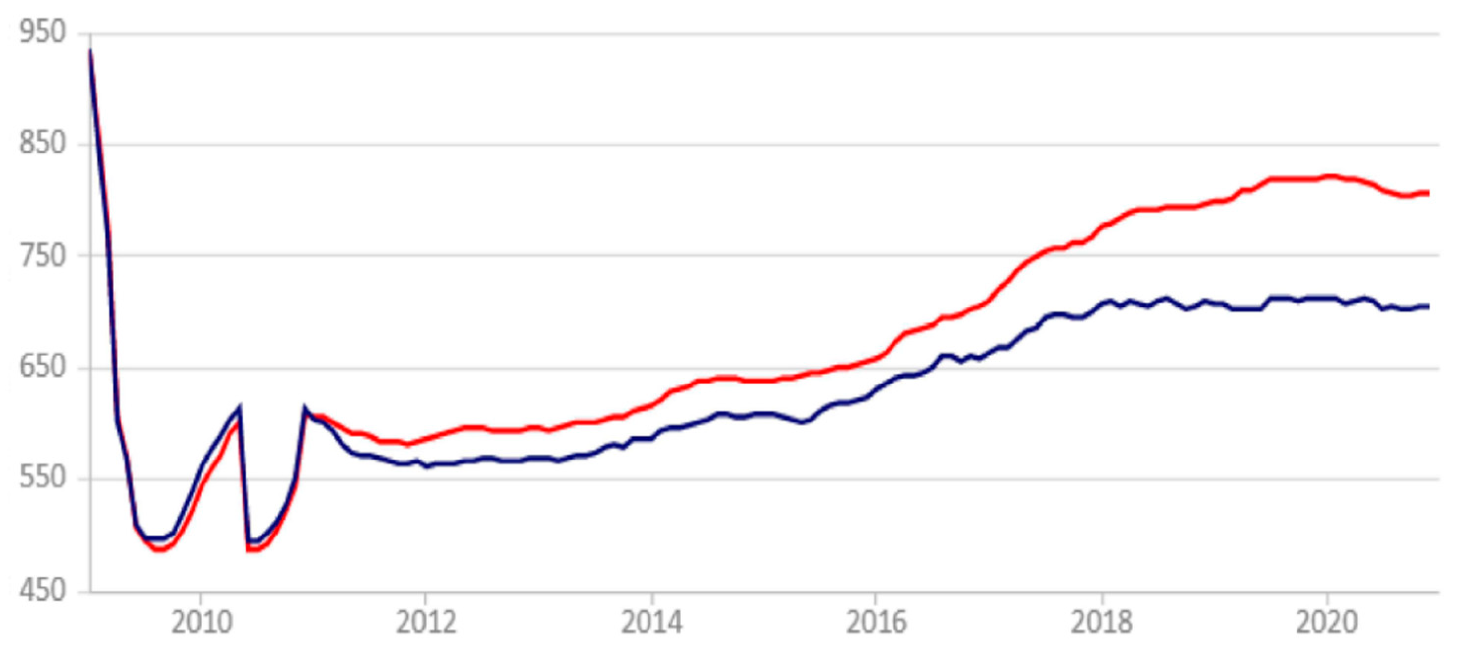
However, the impact of the crisis of 2008–2009 years on the Latvian real estate industry was one of the hardest among others in the Baltic States. Within 2009–2011 Latvia house prices fall almost twice as shown in Figure 3. During the restoration of the real estate business in the 2010–2013 years, the new economic uncertainty was put in place. Due to immigration legislation’s changes (the cancellation of the program of permanent residence permit for the foreign real estate investors) and Latvia’s adoption of the euro on 1 January 2014, uncertainty concerning future real estate demand and house prices had increased dramatically. Therefore, in such “the ideal storm” circumstances, ABC Project Ltd considered several options concerning the project.

Today in the COVID-19 pandemic period, many real estate investors opt to wait, observe, and only in case of positive development invest in the project. It is like several years ago, the investment project “Sun Village” of Latvian real estate developer ABC Projects, Ltd has faced the same challenges whose problems and solutions are presented below in the case study research. As a numerical application, the case study was applied to a typical Latvian real estate project. Nevertheless, the current research can be generalized as a “road map” for similar projects in the EU struggling to attract buyers in the COVID-19 pandemic and post-pandemic periods.

The case study investigated the investment project “Sun Village” of company ABC Project Ltd. into an unfinished real estate project in the Riga region (Latvia) that was acquired by a company Calvus Ltd., which had to sell the unfinished project to cover its debt to the Bank in 2013. The project included the construction of 16 houses, 15 of which were available for sale, however, without proper territory infrastructure in terms of electricity, roads, canalization, etc. Therefore, there were located 16 unfinished houses which were frozen in 2009 due to the global financial crisis.

Sun Village is a residential village in the near suburb of the Latvian capital, in Babite Municipality, which is between Riga and Jurmala, a popular resort. Nearby are located nature reserves and parks of national importance, several lakes, and the Lielupe river. The total area of the land plot is 1500 m². Initially, the new owner ABC Projects, Ltd. company has planned to finish “Sun Village” the project and sell houses as soon as possible. However, in September 2014, Immigration Law amendments increased the threshold for obtaining a residence permit and introduced other conditions and costs (Global Property Guide 2021). Due to immigration legislation’s changes and Latvia’s adoption of the euro on 1 January 2014, uncertainty concerning future demand and prices increased dramatically. ABC Project Ltd was considering several options concerning the project.

The first option was to finish construction and sell finished houses to the buyers as soon as possible (expansion option), the second option was to wait for two years until uncertainty concerning the future real estate sector will become clearer and make investment decision later (deferral option), the third option suggested abandoning the project, namely, to sell immediately the acquired property to other real estate development company (abandon option).

Investors were willing to evaluate each option in terms of profitability. At that time, the company has invested 237,327 € into the purchase of land and 423,833 € in the purchase of the unfinished houses in 2013. All prices are without Latvian Value added taxes. ABC Project Ltd was considering hiring a construction company for project development in case of choosing the first option (expansion option). The construction company’s management had also provided information for the current research on estimated construction costs.

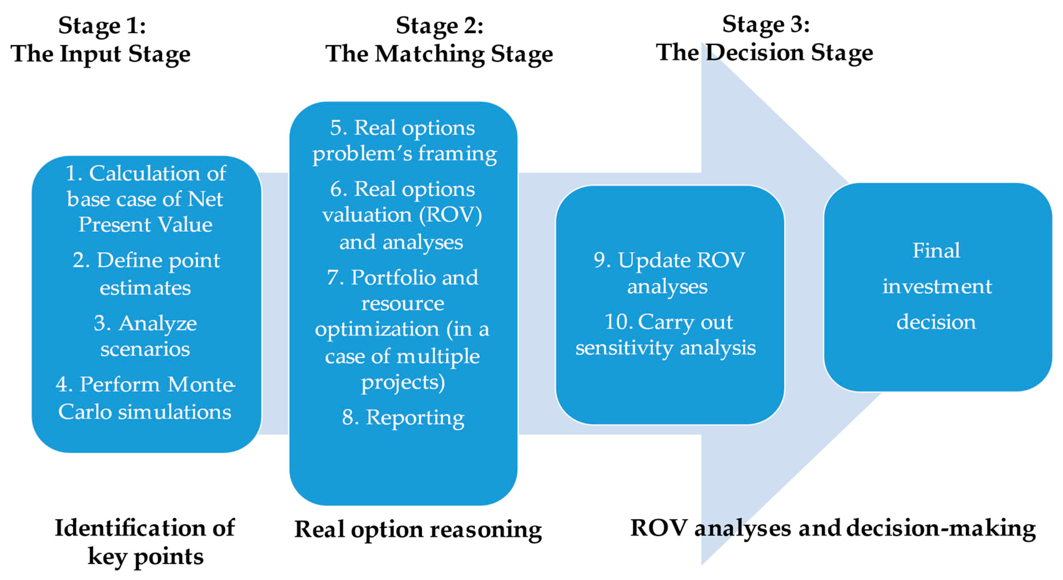
Step one, the discounted free cash flow of the project (DFCF) or present value of a project to be acquired was 5,620,930.44 €. Overall investment into the project was estimated to be 4,912,024.43 €. ABC Project Ltd. founders decided to invest the amount required for project development as a zero percent borrowing. Meanwhile, Latvian Bank stated in the 2014 year that “… in the case of new household loans for house purchase, the annual percentage rate of charge, comprising fees for considering loan applications, loan administration costs, and similar costs, was close to the respective annualized agreed rate” about three percent in 2014 (Latvijas Banka 2014, p. 29). European Central Bank defined an annualized agreed rate as “the interest rate that is individually agreed between the reporting agent and the household or non-financial corporation for a deposit or loan, converted to an annual basis and quoted in percentages per annum” (European Central Bank 2003, p. 13).

Even though the project financing was considered as hundred percent debt financing as free-of-interest charges, the annualized agreed rate adjusted by Latvian corporate withholding tax was employed (Atrill 2020) as the discount rate of free cash flow (FCF) of the current project, and it was equaled 2.55% = 3.00% × (1.00 − 0.15). Thereby, the net present value (NPV) of the investment project as estimated through discounted cash flow approach was 708 906,01 €. The internal rate of return (IRR) of the project was estimated at 9.21% and corresponded with the expected required rate of return of the founders of the company.

Even though in other European countries such IRR value is too low for a real estate investment, the owners did not reject a project. Although the IRR and the NPV methods give consistent accept-reject decisions, they may not rank projects identically. In general, the NPV method is theoretically superior (Titman et al. 2014) and the investors were satisfied with a positive NPV result.

Next, the deferral option to wait for two years until uncertainty concerning the future real estate sector will become clearer and make investment decisions later had to be explored. Thus, in Step two, uncertain variables that influence the bottom line (DFCF value) were estimated which are discussed next in terms of prices and expenses. Step three, pessimistic, optimistic, and most likely scenario developments affecting future cash flows were analyzed. The optimistic, most likely, and pessimistic real estate square meter prices were provided by ABC Project Ltd management based on their managerial assumptions. The pessimistic scenario means that real estate prices would decrease by approximately 41.6 percent by the end of 2016. The optimistic scenario assumed that prices on real estate objects would continue to grow.

Therefore, for the first 2014 year’s revenues forecast assumptions were provided as follows: pessimistic—1273 €; optimistic—1624 €, and most likely 1478 €; for second 2015-year forecast assumptions were provided as follows: pessimistic—1068 €; optimistic—1624 €, and most likely 1478 €; and for third 2016 year: pessimistic—863 €; optimistic—1624 €, and most likely 1478 €.

Step four, Monte Carlo simulation was done because the standard DFCF model produces only one static estimated result, not taking into account the future events that highly affect forecasted cash flow. According to Cobb and Charnes (2007), the preciseness of the distribution is increased, when more simulation trials are executed. Therefore, Oracle Crystal Ball (OCB) software was used to estimate project return volatility. Triangle distribution was used for the expected square meter price variation assumptions mentioned above. The construction company assumed that construction costs may increase or decrease by approximately 5 percent. Thus, OCB software was used again to find a normal distribution of material costs.

The management of ABC Project, Ltd also provided their expectation on the volatility of additional administration expenses including management salary and associated taxes as well as other operating expenses. Inflation trends on construction costs were also taken into account in the study.

Then, the OCB software simulation ran 2,000,000 times. At each simulation, OCB has randomly taken numbers following probability distribution on square meter’s price, construction costs, administrative and operating expenses that were set and calculated previously. Besides, the present value of future cash flows for the base case DFCF model was used as the initial underlying asset value in real options modeling according to Mun (2002).

Preliminary implied volatility of the DFCF of Sun Village project was forecasted at 62.72 percent (Čirjevskis and Tatevosjans 2015, p. 56). Today in the 2021 year, it should be admitted that the assumptions on implied volatility were unnecessarily radical. The Latvia house prices have been stabilized after the boom and bust of 2009–2013 years and further have demonstrated moderate volatility dynamic as shown in Figure 3.

In this vein, having explored the value of deferral option for the period from April 2014 until May 2016 of this project, the volatility of DFCF (period) has been re-estimated according to the recently published date of Global Property Guide (2021) as given in

Table 3. Quarterly house prices in Latvia: average price of a standard type of apartment in Riga (Euro per sq. m.) Source: Global Property Guide (2021).

Years	Q1	Q2	Q3	Q4
2014	640 €	-	-	-
2013	637 €	640 €	640 €	641 €
2012	592 €	595 €	595 €	594 €
2011	609	592	571	585
2010	612 €	493 €	488 €	521 €
2009	934 €	849 €	494 €	576 €

.

To measure the volatility of DFCF, the coefficient of variation (CV) was applied to expresses the standard deviation of DFCF as a percentage of what is being measured relative to the forecast of DFCF’s mean. “In investing, the coefficient of variation is used to measure the volatility (represented by the standard deviation) to the expected return on an investment” (Farlex Financial Dictionary 2009, p. 1). For the period of the “Sun Village” project, the average house price in Latvia was 614.19 € per sq. m., and the standard deviation of the house price for that period was 105.05 €. Thereby, the volatility of DFCF was at 17.10% which is significantly lower than the preliminary volatility estimation of the “Sun Village” project.

Step five, the company had to consider several options regarding the project. One of these options is to wait (deferral option) two years until uncertainty concerning the project will decrease and decide and the other is to sell (abandonment option) acquired property to another development company. In case the company decides to finish construction (expansion option), it would also have to adapt the territory in terms of electricity, roads, canalization. Moreover, the company would construct an additional administration house to serve this property in the future in terms of security, small repairs, and other miscellaneous services.

Step six. To justify the proposition and to provide an estimation of managerial flexibility’s value by putting off an investment decision for two years till May 2016, three ROV methods were employed as follows: Black-Scholes option pricing model (

Table 4. Black-Scholes option-pricing model’s input variables.

Present value of expected cash flows of the project (So)	5,620,930.44€
Cost of investment or exercise price (E)	4,912,024.43€
The risk-free rate of return (r)	3.00%
Time to expiration in years (T)	2.0
The volatility of PV of FCF (σ)	17.10%

Source: Developed by the author.

and

Table 5. Black-Scholes option-pricing model’s variables and results.

Option Sub-Variables	Data	Option Sub-Variables	Data
T =	2.00 years	d1 =	0.9265
S0/E =	1.1443	N(d1) =	0.8229
ln(S0/E) =	0.1348	d2 =	0.6847
variance/2 =	0.0146	N(d2) =	0.7532
[risk-free rate + variance/2] × T =	0.0892	−rT =	−0.0600
the square root of variance =	0.1710	e−rT =	0.9418
the square root of T =	1.4142	S0 x N(d1) =	4,625,478.72 €
(square root of variance) × (square root of T) =	0.2418	K × e−rT × N(d2) =	3,484,367.01 €
		Real option value: C	1,141,111.71 €

Source: Developed by the author.

), Monte Carlo simulation (

Table 6. Monte Carlo pricing of call option’s parameters and the result.

European Call Option	C
Present value of expected cash flows of the real estate project (So)	5,620,930.44 €
The investment required to execute the real estate project (E)	4,912,024.33 €
Time to expiration (T)	2.0 years
Real estate project uncertainty or volatility (σ)	17.10%
Risk-free rate (Rf)	3.00%
Number of steps	6
Number of simulation	1,000,000
European Call option price (deferral option)	1,141,609.78 €

Source: Developed by the Author.

), and binomial option pricing model (

Table 7. Parameters of the binominal option pricing model lattices.

time increment (years)	$\mathsf{\delta }\mathrm{t}=\frac{\mathrm{t}}{\mathrm{N}}$ = 0.33
up factor (u)	$\mathrm{u}={\mathrm{e}}^{\mathsf{\sigma }\surd \Delta \mathrm{T}}=\frac{1}{\mathrm{d}}$ = 1.104
down factor (d)	$\frac{1}{\mathrm{u}}$ = 0.906
risk-neutral probability (p)	$\mathrm{p}=\frac{{\mathrm{e}}^{\mathrm{r}\Delta \mathrm{T}}-\mathrm{d}}{\mathrm{u}-\mathrm{d}}$= 0.526

Source: Developed by the author.

and Figure 4) by assuming that all methods would give approximately the same result. Following input variables were required for real options valuation by Black-Scholes option pricing model as shown in Table 4.

As can be observed in Table 4, having applied Equation (1) of the Black-Scholes option pricing model, the value of the project (eNPV) may increase by 1,141,111.71 €, in the case of waiting for two years (deferral option) before making an investment decision.

Then, applying the Monte Carlo simulation, Excel forecasted the call option value for the “Sun Village” project calculated as shown in Table 6. The option life was divided into six time steps, the same as for binominal lattices below, and the number of simulations was 1,000,000 times. The simulation results from a custom-made spreadsheet show a real option value of 1,141,609.78 €.

As can be observed from Table 4 and Table 5, in the case of waiting two years before making an investment decision (deferral option), the NPV of the project may increase to 1,141,111.71 € according to the BSOP approach and 1,141,609.78 € according to the MCS approach and, thus, additionally adding the value more than one and a half million EUR.

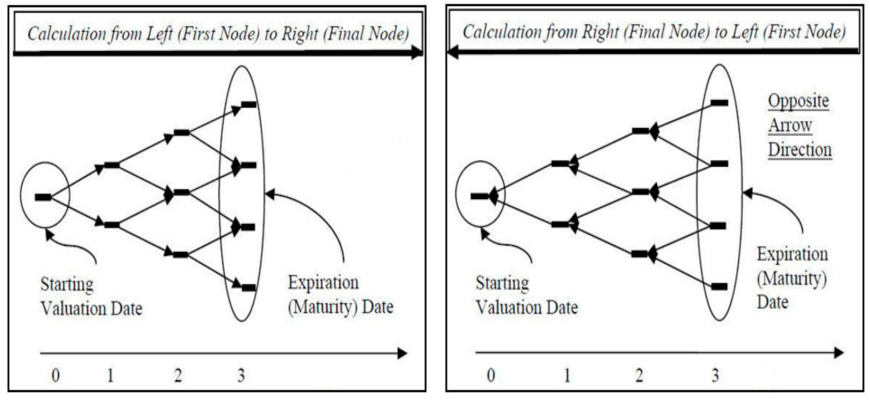
To estimate the value added that may be provided by postponing investment decisions for two years (deferral option), binomial option pricing model approaches have been used as shown in Figure 4. The underlying lattice (event tree) was constructed by beginning with the starting upper node and proceeding left to right till options expiration. Then, the real option valuation lattice was constructed in the opposite direction backing to the starting down node. For descriptive appeal, both lattices were merged into one lattice as shown in Figure 4.

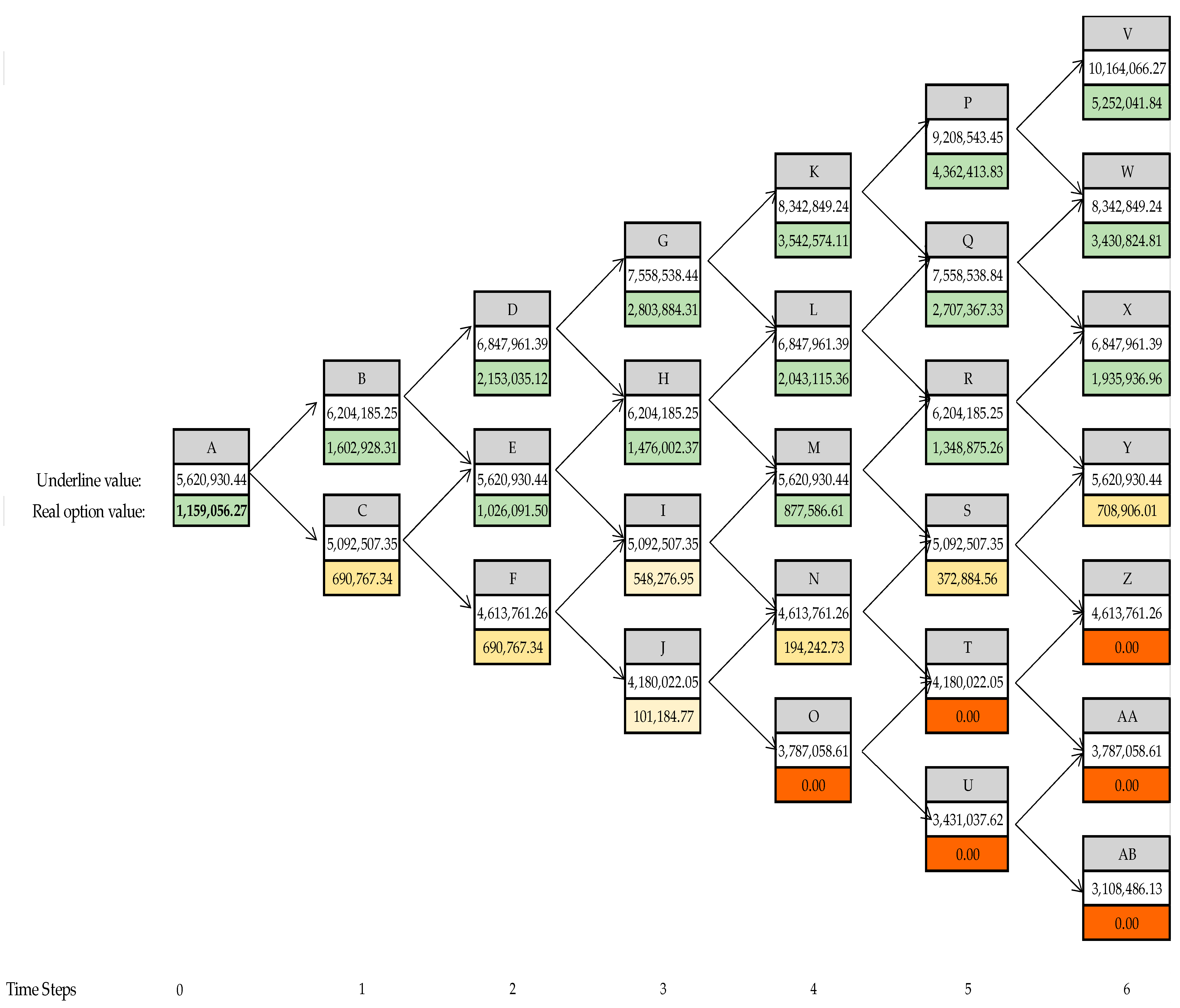
Zero steps in Figure 4 represent the current period of the project (April 2014 year). The time till expiration was divided into six-time increments for the decision tree construction. The recombining binomial lattices parameters are given in Table 7.

One-time increment represents 0.33 of a year. At each time step, the previous tree cell is multiplied by the up and down factor until six steps are made. At step number six possible project values in two years were calculated and can be observed in Figure 4. Up and down factors were used as a multiplier during the one-time increment step in a binomial tree; up factor (u) = 1.104 and down factor (d) = 0.526. The present value of the expected DFCF is estimated at 5,620,930.44€ and therefore is used as a starting point in the binomial tree.

Then backward induction’s steps were required to identify if the deferral option to wait for two years would be in the money. The results for each of these potential outcomes were calculated by deducting initial investment from each of these results. In cases when there were losses, they were shown as a zero since in these cases options would not be exercised. The values of intermediate nodes for each time step increment during this process was calculated by using Excel as follows: intermediate node value = (risk-neutral probability*(previous up factor cell) + (1-risk-neutral probability)*(previous down factor cell))*EXP(-risk-free rate of return*time increment) = (0.526*(previous up factor cell) + (1-0.526)*(previous down factor cell))*EXP(-3.00%*0.33) as shown in Table 7 and Figure 4.

Now, the result of the BOPM simulation can be compared with the results of BSOP and MCS. Received with binomial approach real option value differs from that suggested by Black-Scholes and Monte Carlo approach by approximately 1.5 percent: BSOP—1,141,111.71€, MCS –1,141,609.78 € versus BOPM—1,159,056.27 €. Such difference appeared due to a relatively low number of time step increments producing just six possible investment outcomes in BOPM as can be observed in Figure 4. On the other hand, BOPM provides a more straightforward understanding and visualizes how project uncertainty represented by volatility influences option value during its lifetime.

In point of fact, in case of waiting for two years before making a further investment decision, the value of project NPV might increase to about from 708,906 € to 1,141,500 € according to BSOP and MCS approaches to 1,159,000 € according to BOPM and, therefore, add a value about a half of million € in comparison with a static NPV 708,906 €. Therefore, from the discussion above, it can be determined that if the investors would indeed make a value-maximizing decision over the next two years, it would have augmented the value of the Sun Village project by about 450,000 € and the ROV premium would be 20.6% ([eNPV-NPV]/NPV) (Mun 2002).

Because the “Syn Village” project did not depend on other projects of company ABC Project Ltd and the portfolio resource optimization was not required, seven–nine steps were missed in the research.

Step ten. Luehrman suggested performing sensitivity analysis after the real options valuation as it will serve as a further strategy as the project develops Luehrman (1998). In this vein, the conduction of sensitivity analysis has shaped the decision-making on value maximization of real estate development project “Sun Village”. Sensitivity analysis was produced by the OCB simulation. It was observed that the variance of free cash flows (FCF) is mostly affected by the first and second house type prices—by 60.7% and 17.4% consequently. Construction costs variation has affected FCF by 14.4%. Administration and operating expenses have almost no effect on free cash flow variation. However, Brealey and Myers criticized the sensitivity analysis and argued that the disadvantage of the analysis relates to the fact that it does not account for interrelated underlying variables (Brealey and Myers 2000).

Thus, the case study has provided a better understanding of phenomena of real options hybrid applications on concrete real estate project in economic uncertainty context, helped to make a value-maximizing decision by choosing deferral option, and the research result can be generalized in the current COVID-19 pandemic period for similar real estate projects as discussed below.

5. Discussion and Contributions

Real options reasoning is a conceptual approach to investment that considers the value of the right to make future choices under uncertain conditions (McGrath and Nerkar 2004, p. 1) can be employed by real estate developers. Lucius argued, “as promising as the real options approach appears in the field of real estate research and as convincing as the academic findings may be, the challenge lies in the transfer to practical application in the field of investment valuation” (Lucius 2001, p. 78). The current paper contributes to this empirical request.

Several scholars’ studies have demonstrated that both the Monte Carlo simulation and the binomial models converge to the Blacks-Scholes option pricing value (Hon 2013). In this vein, the paper contributes to this conversation by justifying the Hon’s (2013) arguments with the fresh empirical result. Moreover, research evidence that the binomial method makes the calculations visible and strategically flexible, so the results can be easily understood and communicated to practitioners, whereas Black- Scholes model gives higher accuracy.

The paper extends the empirical real option application discussion in the real estate industry by bringing real options models closer to the practitioners. This is done through developing a “step-by-step” practical application model through which real estate managers can easily calculate their optimal decisions.

This paper enriches the discussion about the current literature on real options in real estate and examines practical implementation problems associated with the real options approach. Thereby, the paper has provided new insights into capital budgeting decision-making practices and a new decision-making framework based on real options. The paper shows that the application of real options is a flexible decision management tool and being coupled with three real options valuation techniques (BOPM, BSOP, MCS) has a significant advantage. Depending on the specific situation, practitioners might require supplementary assistance from consultants to estimate the real options models’ input parameters.

Ragozzino et al. argued that financial economics and strategy have worked in quasi-independent ways over the years and two fields of research might be brought closer together toward the development of a real-option agenda that can be fruitful to various stakeholders (Ragozzino et al. 2016, pp. 437–38). The paper has also contributed to this research agenda. This paper bridges the gap between theory and practice in real option application adoption in the decision-making of a real estate business. Ragozzino et al. argued that “the real options approach holds tremendous potential for academics and practitioners. Yet, empirical work to date has not been able to bring conclusive evidence on the theory’s merits and a normative framework…” (Ragozzino et al. 2016, p. 437).

Therefore, the paper’s contributions are two-fold: on the theory side, the paper demonstrates how to use more realistic real options hybrid models (Marques et al. 2021a); and, on the practical side, disseminates the knowledge of real options application in real estate organizations. Regarding managerial implications, real estate management should actively seek (active learning) to clear the uncertainty by conducting focused market surveys. “Without growth, it’s really hard to deliver good returns. When markets get stuck, that’s when you can see the difference between brilliant and mediocre managers” (PwC and the Urban Land Institute 2021, p. 64).

6. Conclusions, Limitations, and Future Work

The case study research has justified the proposition “Real options valuation approach is an opportunity to adapt real estate investments to changing circumstances and to decide to what extent it is worth to develop the real estate project and when to sell the real estate”. The paper illustrates how the hybrid methods’ combination of BOPM, BSOP, and MCS ROV models can contribute to the economic analysis of investments in new projects in the real estate market, supporting the process of decision-making by managers. When it comes to comparative appropriateness of different methods of real options valuation, the BSOP model and MCS are exact, quick, but are difficult to explain to practitioners because they require highly technical stochastic calculus mathematics (Mun 2002). BOPM lattices are in contrast, easy to explain and implement, but require significant computing power and time-steps to obtain good approximations (Mun 2002).

There are three categories of limitations of the ROV research. The first deals with the validity of data provided to the researcher. It must be noted that the results of the analysis are only as good as the figures behind them. All conclusions and subsequent recommendations made are based on the premise that the financial data provided to the researcher represent a realistic situation of the business. In case the data are subject to a change (which is most likely due to the continual nature of ROV), the analysis becomes void. Thus, the recommendations are valid at the time of research; any update of data after the mentioned date is beyond the scope of this paper.

Second, the analytical approach used is subject to certain limitations. Real options analysis applied was that of risk-neutral probabilities—inevitably this approach has to make certain assumptions most of which are based on implied volatility outlined in Table 1. Any estimation includes assumptions. Since they have a major impact on the implied volatility estimation, financial results should be interpreted and perceived as approximations only.

Last but not least, it should be stressed that due to the mathematical complexity involved, real options problems are far better solved using specialist software. In this vein, to align management incentives and to develop user-friendly real options software (Marques et al. 2021a), practitioners can use other packages such as the DerivaGem software that accompanies Hull publication (Hull 2018) and that can be found online free of charge that can be also a good solution for calculating real options value (Marques et al. 2021b).

Finally, the real estate investment decisions of firms are, in most cases, taken within a strategic competition with other firms in the industry, where the competitive actions of one company affect the decisions of the others (De Almeida et al. 2019). In this vein, having contributed to the literature by bridging three real options valuation approach in the cohesive whole model in the current paper, the future work can provide more robust economic analyses and interpretations regarding the demand for real estate, showing quantitatively how competition can impact strategic decisions (De Almeida et al. 2019).

Furthermore, a least squares Monte Carlo simulation-based real options (Longstaff and Schwartz 2001) should be discussed in comparison with the Black and Scholes, Monte Carlo, and binomial trees. “…By its nature, simulation is a promising alternative to traditional finite difference and binomial techniques and has many advantages as a framework for valuing, risk managing, and optimally exercising American option” (Longstaff and Schwartz 2001, p. 114). Gamba (2003) suggested that this approach is more suited to evaluate complex investments with many interacting options.

This simulation method has been recently applied by Dehghan-Eshratabad and Albadvi (2018) to value start-ups by venture capitalists in the first round of financing. Zheng and Negenborn (2017) applied the simulation for a Chinese steel cargo terminal investment decision in a competitive setting with uncertainty. Thus, least squares Monte Carlo simulation-based real options (Longstaff and Schwartz 2001) can overcome some limitations of traditional ROV approaches. Hence, this is a promising area for future research.