
A Comparison of Artificial Neural Networks and Bootstrap Aggregating Ensembles in a Modern Financial Derivative Pricing Framework


Abstract
1. Introduction
2. Methodology
2.1. The Piterbarg Framework
2.2. The Piterbarg PDE
2.3. Solutions for European Call Options in the Piterbarg Framework
2.4. Neural Network Modeling Approaches
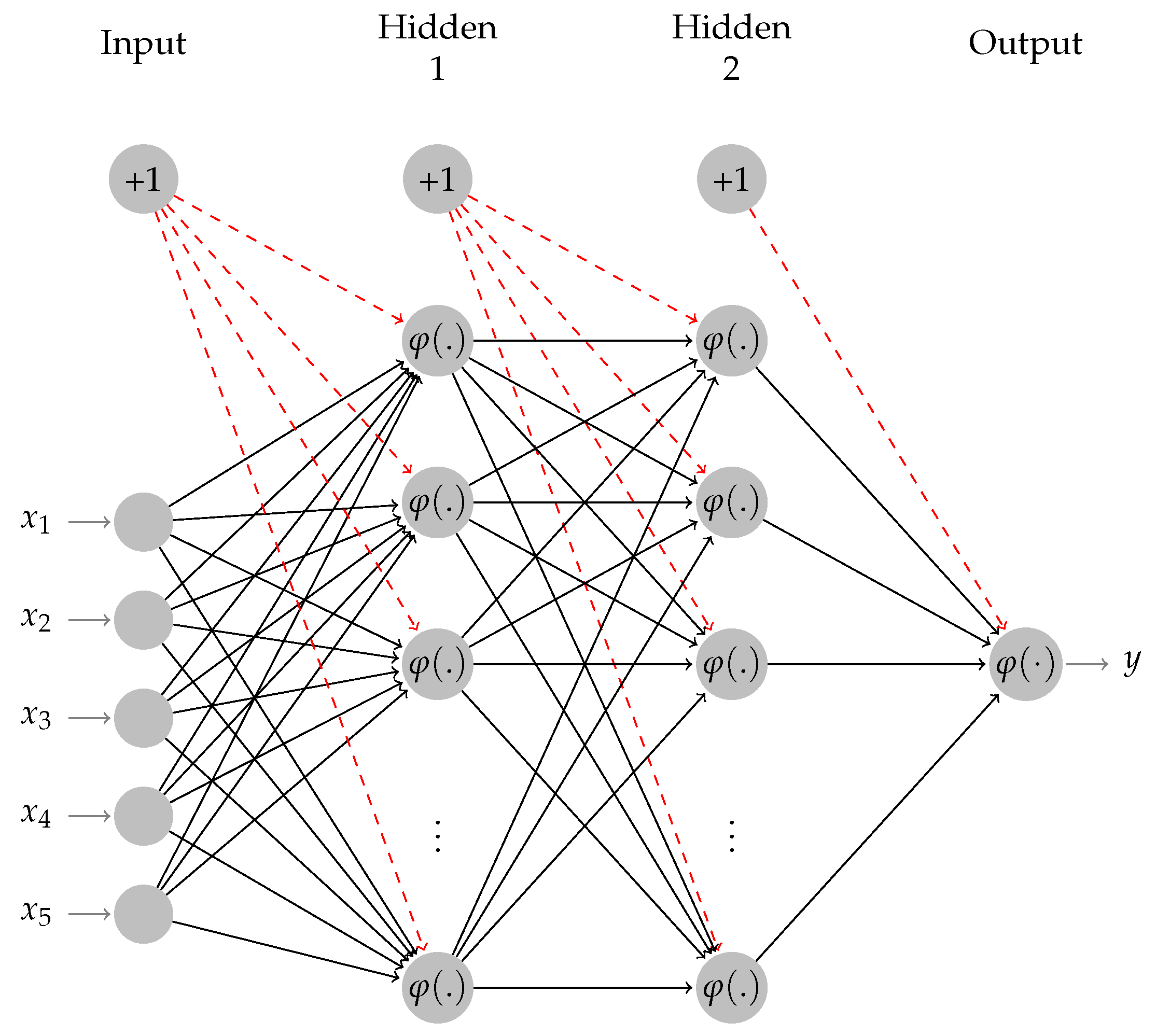
2.4.1. Artificial Neural Networks
2.4.2. Ensemble Methods
3. Data Generation and Base Learner Configuration
3.1. Training Data
3.2. Testing Data
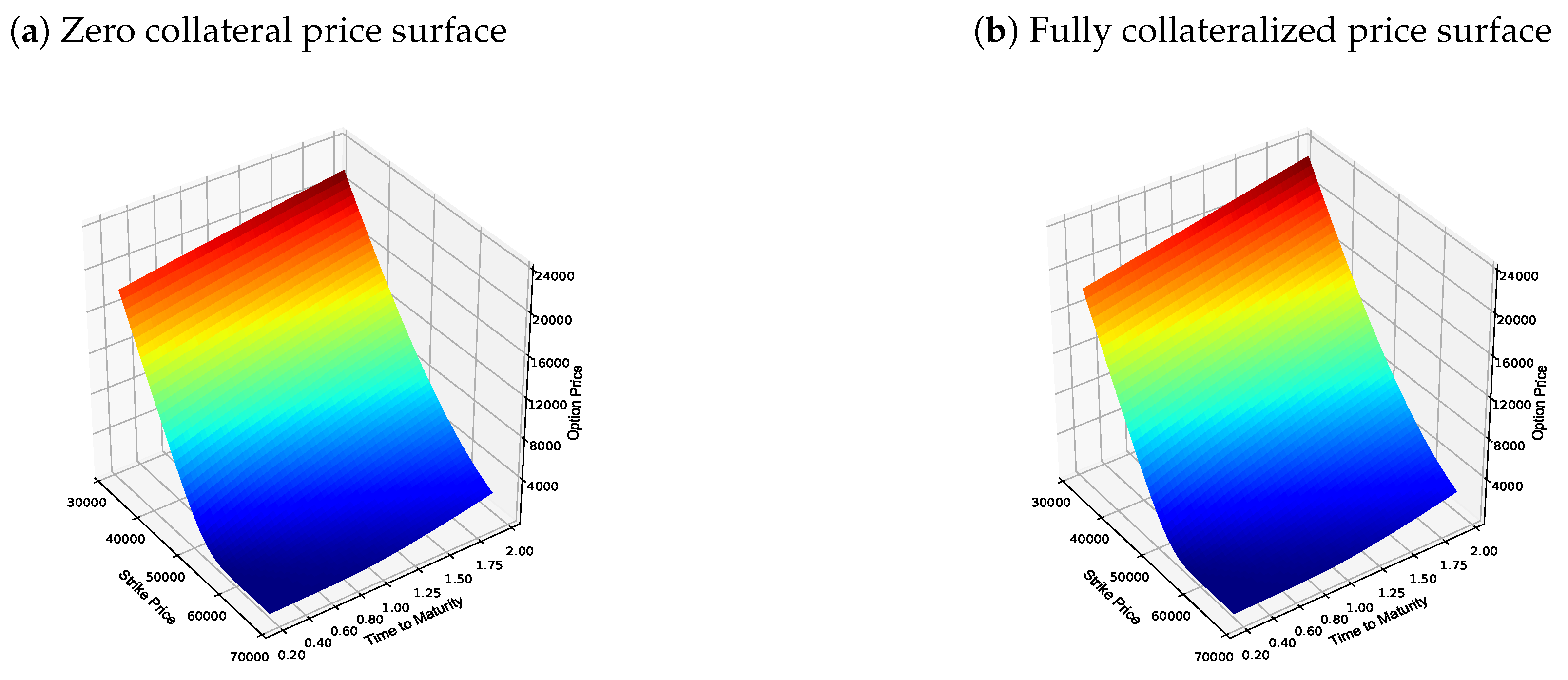
- If zero collateral trades were considered, it was assumed that the implied volatility surface was constructed using zero collateral trades;
- If fully collateralized trades were considered, it was assumed that the implied volatility surface was constructed using fully collateralized trades.
3.3. Base Learner Configuration
4. Results
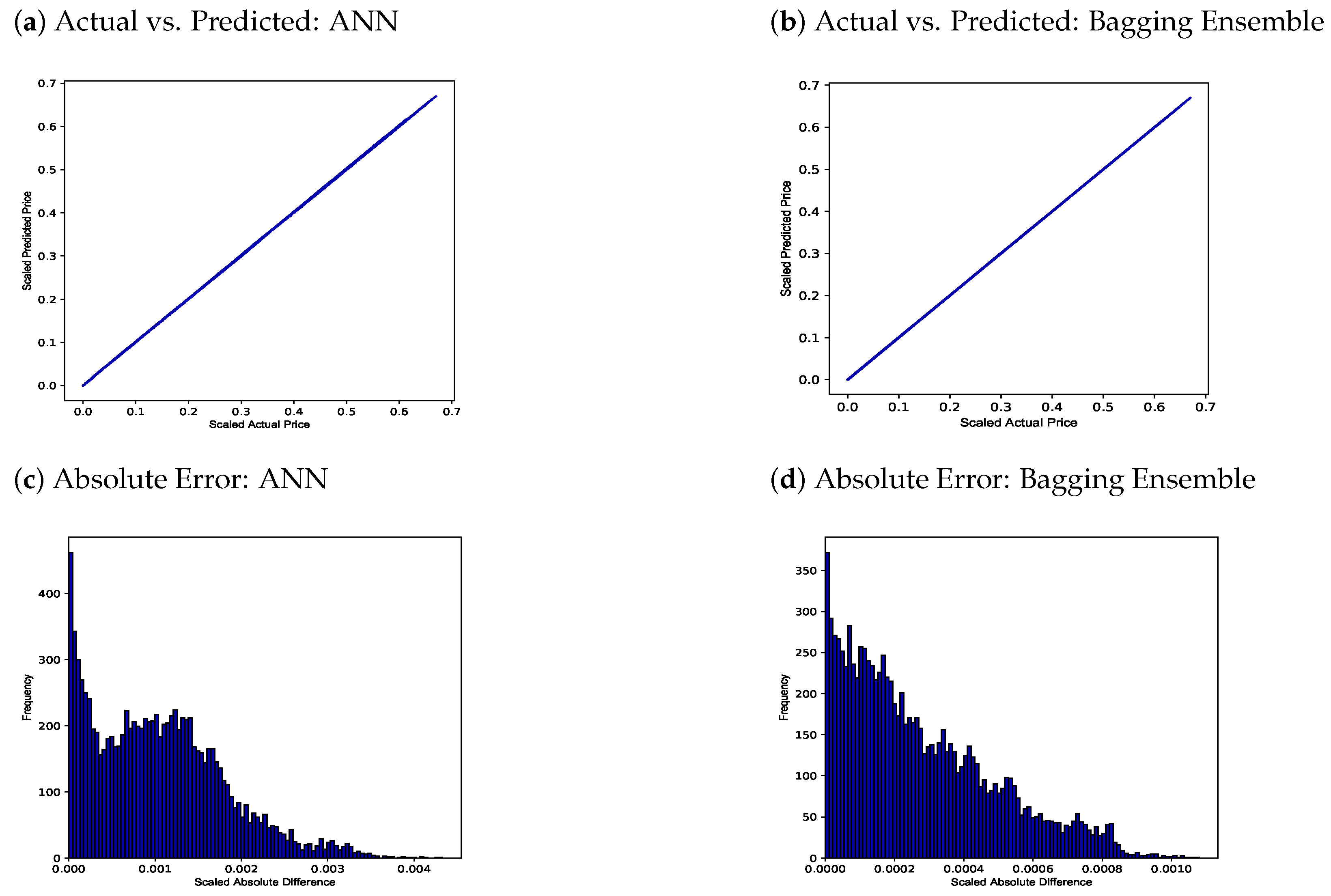
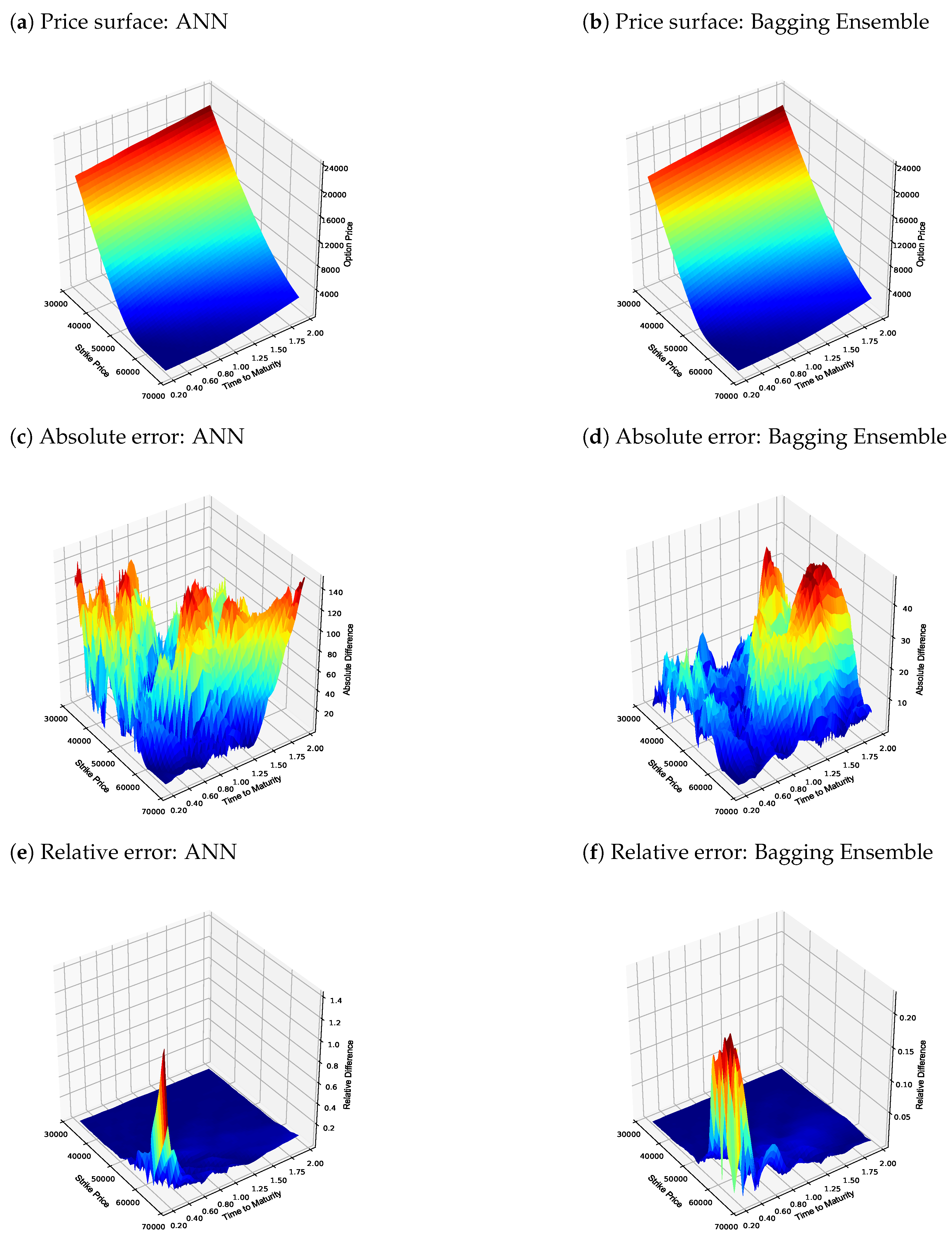
4.1. Zero Collateral Numerical Results
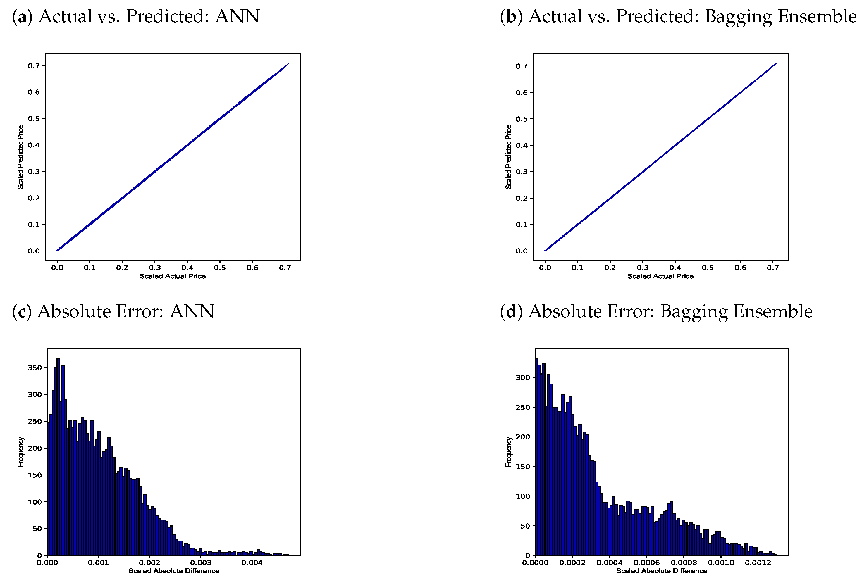
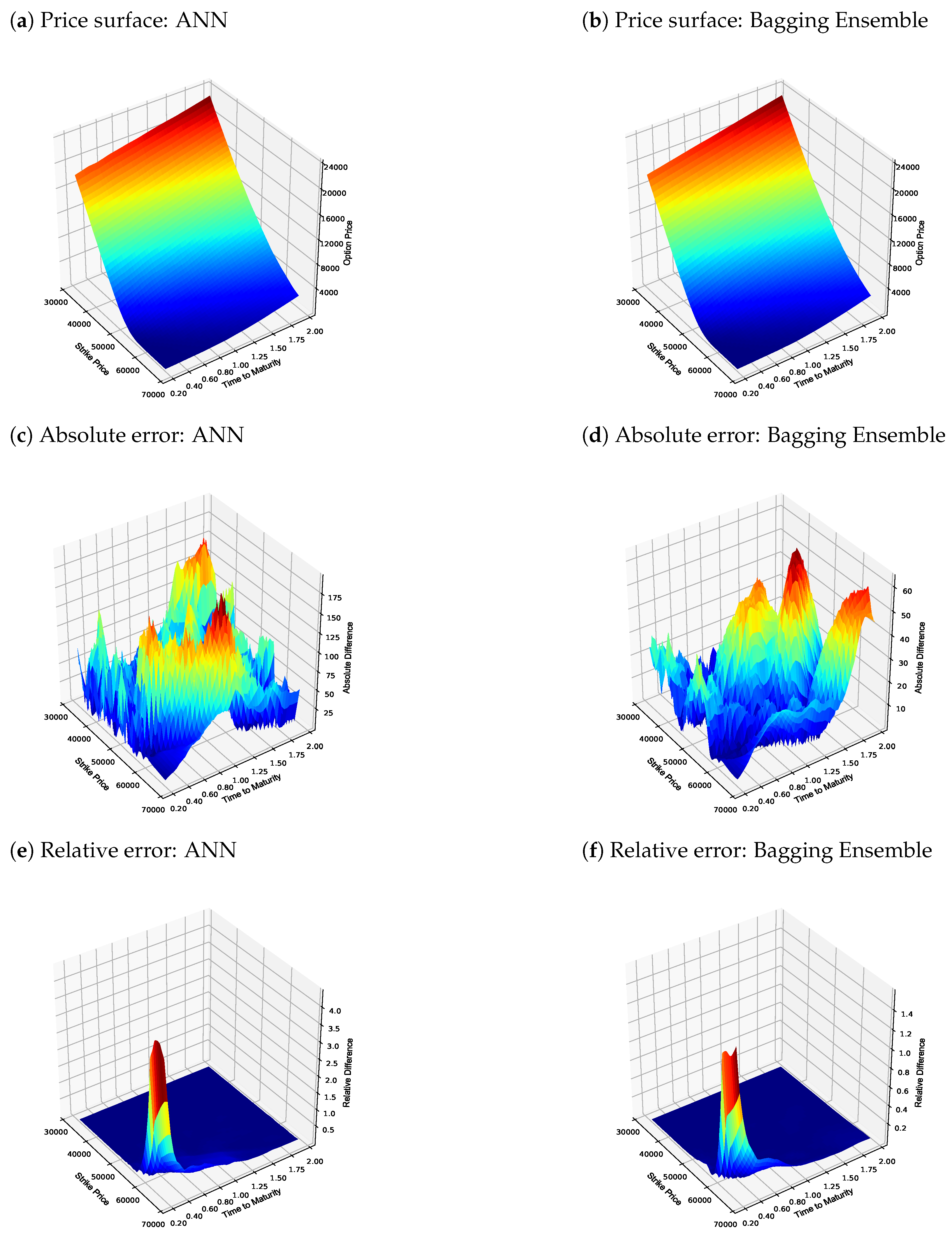
4.2. Fully Collateralized Numerical Results
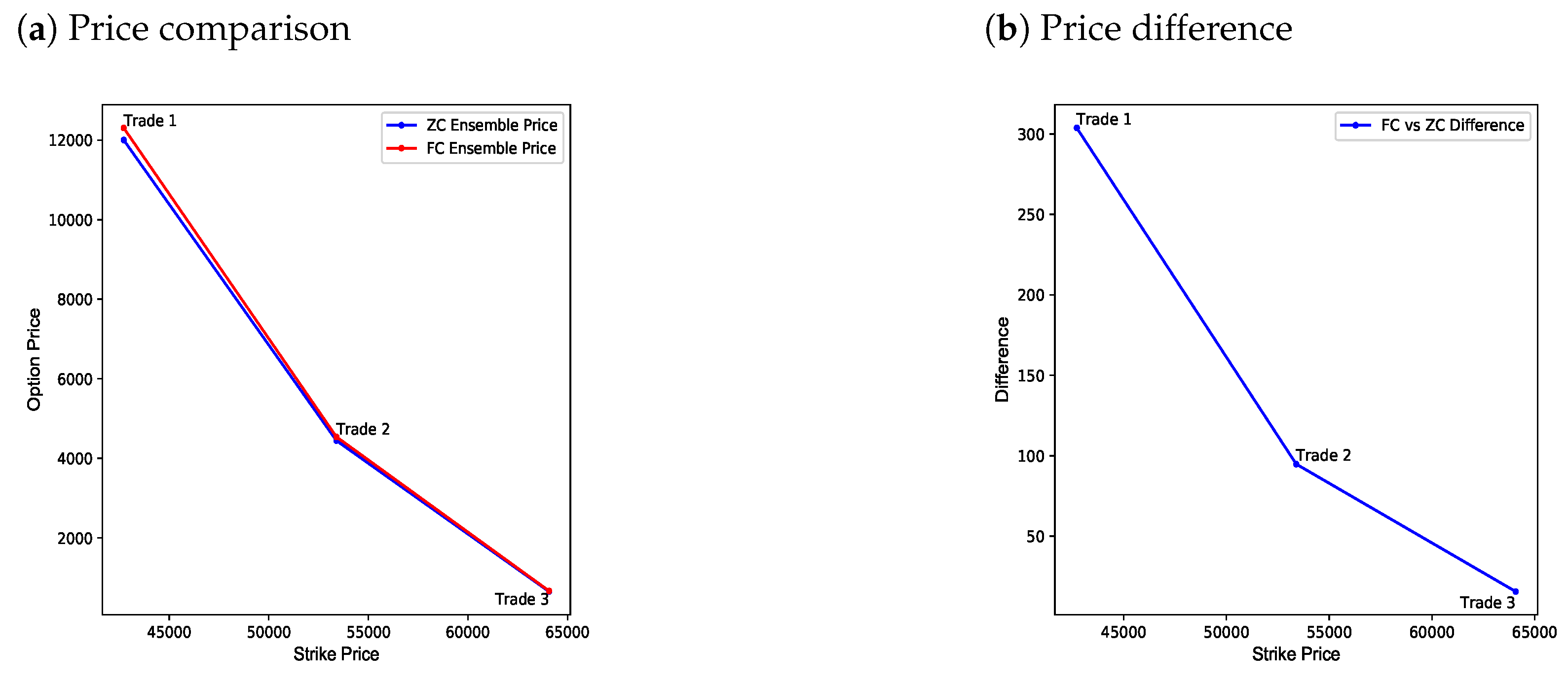
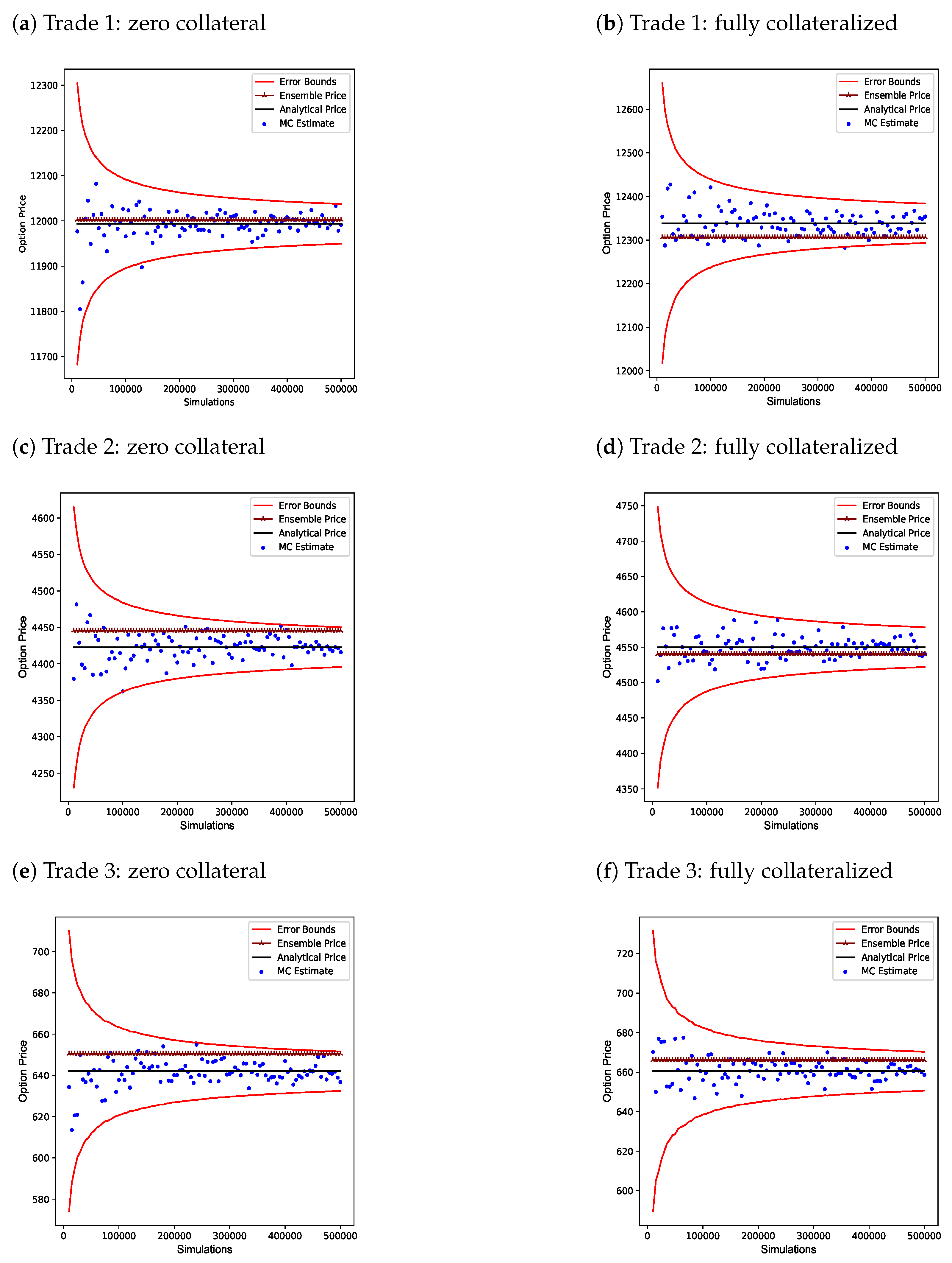
4.3. Numerical Results: Bagging Ensemble vs. Monte Carlo Simulation
- The stochastic process of the underlying asset follows a geometric Brownian motion;
- Constant interest rates were assumed;
- The underlying asset does not pay any dividends;
- Trades are European in nature;
- Trades are devoid of any friction costs;
- An Actual/365 day-count convention is used;
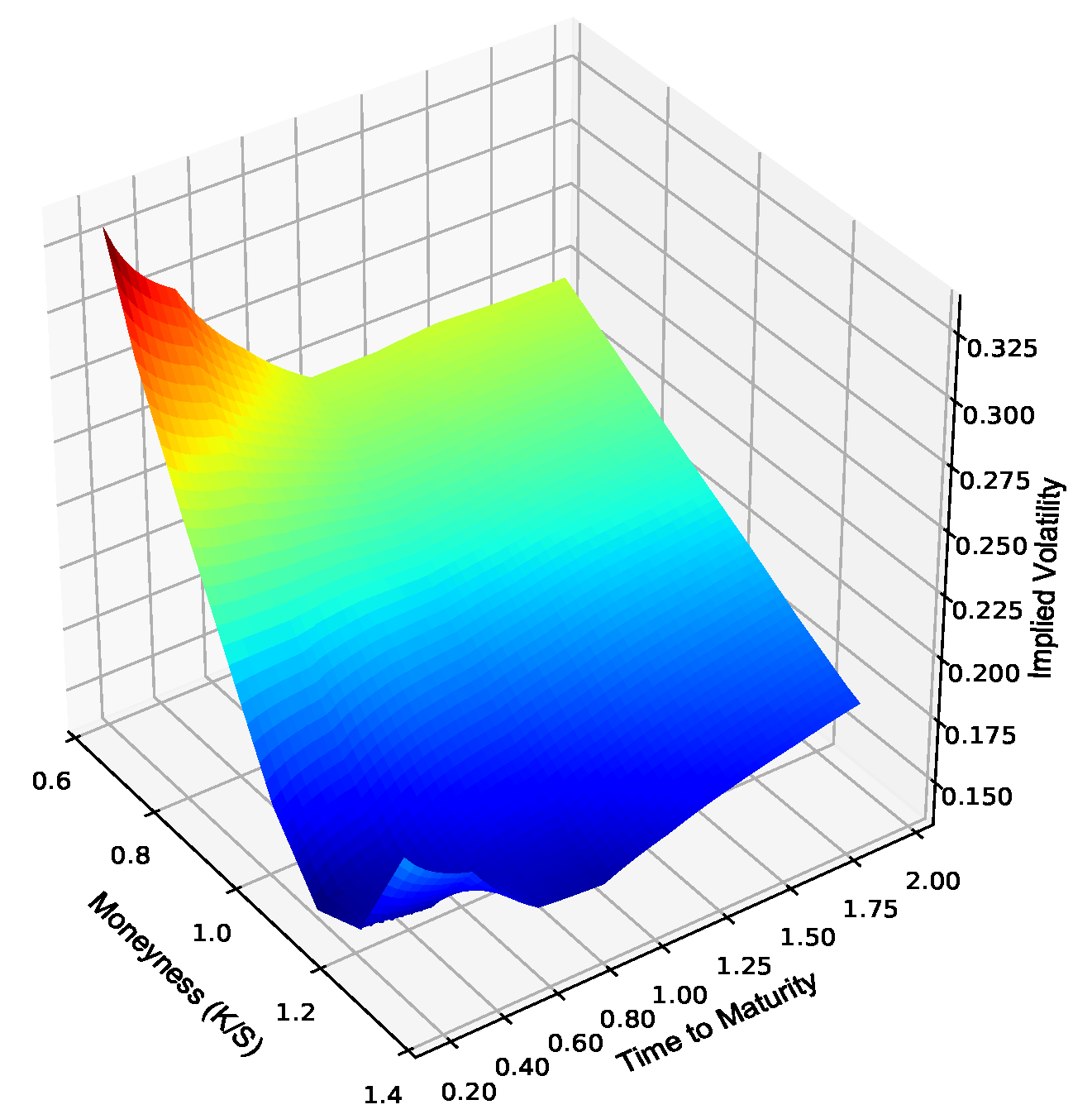
- The implied volatility parameters obtained from the volatility skew dated 9 April 2019 were assumed to be constructed using either zero collateral or a fully collateralized trades, depending on which type of trade was considered;
- We assumed vanilla options only.
- Given the relation in Equation (2), the price of a zero collateral European call option must be less than that of a fully collateralized European call option for any trade;
- For the bagging ensemble to be a viable alternative to a Monte Carlo simulation, it must be shown that the numerical accuracy of the bagging ensemble is within the three standard deviation error bounds of Monte Carlo simulation estimates for a reasonable number of simulations.
5. Conclusions
Author Contributions
Funding
Institutional Review Board Statement
Informed Consent Statement
Data Availability Statement
Acknowledgments
Conflicts of Interest
References
- Bennell, Julia, and Charles Sutcliffe. 2004. Black–Scholes Versus Artificial Neural Networks in Pricing FTSE 100 Options. Intelligent Systems in Accounting, Finance and Management 12: 243–60. [Google Scholar] [CrossRef]
- Bishop, Christopher M. 2006. Pattern Recognition and Machine Learning. Berlin/Heidelberg: Springer. [Google Scholar]
- Black, Fischer, and Myron Scholes. 1973. The Pricing of Options and Corporate Liabilities. Journal of Political Economy 81: 637–54. [Google Scholar] [CrossRef]
- Breiman, Leo. 1996. Bagging Predictors. Machine Learning 24: 123–40. [Google Scholar] [CrossRef]
- Chollet, François. 2015. Keras. Available online: https://github.com/fchollet/keras (accessed on 21 November 2020).
- Culkin, Robert, and Sanjiv R. Das. 2017. Machine Learning in Finance: The Case of Deep Learning for Option Pricing. Journal of Investment Management 15: 92–100. [Google Scholar]
- Cybenko, George. 1989. Approximation by Superstitions of a Sigmoidal Function. Mathematics of Control, Signals and Systems 2: 303–14. [Google Scholar] [CrossRef]
- De Prado, Marcos Lopez. 2018. Advances in Financial Machine Learning. Hoboken: John Wiley & Sons. [Google Scholar]
- Garcia, René, and Ramazan Gençay. 2000. Pricing and Hedging Derivative Securities with Neural Networks and a Homogeneity Hint. Journal of Econometrics 94: 93–115. [Google Scholar] [CrossRef]
- Goodfellow, Ian, Yoshua Bengio, and Aaron Courville. 2016. Deep Learning. Cambridge: MIT Press. [Google Scholar]
- Hamori, Shigeyuki, Minami Kawai, Takahiro Kume, Yuji Murakami, and Chikara Watanabe. 2018. Ensemble Learning or Deep Learning? Application to Default Risk Analysis. Journal of Risk and Financial Management 11: 1–14. [Google Scholar] [CrossRef]
- Hornik, Kurt, Maxwell Stinchcombe, and Halbert White. 1989. Multilayer FeedForward Networks are Universal Approximators. Neural Networks 2: 359–66. [Google Scholar] [CrossRef]
- Hunzinger, Chadd B., and Coenraad C. A. Labuschagne. 2015. Pricing a Collateralized Derivative Trade with a Funding Value Adjustment. Journal of Risk and Financial Management 8: 17–42. [Google Scholar] [CrossRef]
- Hutchinson, James M., Andrew W. Lo, and Tomaso Poggio. 1994. A Nonparametric Approach to Pricing and Hedging Derivative Securities via Learning Networks. The Journal of Finance 49: 851–89. [Google Scholar] [CrossRef]
- Kingma, Diederik P., and Jimmy Ba. 2014. Adam: A Method for Stochastic Optimisation. Available online: https://arxiv.org/abs/1412.6980 (accessed on 4 January 2021).
- Levendis, Alexis, and Pierre Venter. 2019. Implementation of Local Volatility in Piterbarg’s Framework. In International Conference on Applied Economics (ICOAE 2019): Advances in Cross-Section Data Methods in Applied Economic Research. Cham: Springer, pp. 507–21. [Google Scholar]
- Liu, Shuaiqiang, Cornelis W. Oosterlee, and Sander M. Bohte. 2019. Pricing Options and Computing Implied Volatilities using Neural Networks. Risks 7: 1–22. [Google Scholar] [CrossRef]
- Merton, Robert C. 1973. Theory of Rational Option Pricing. The Bell Journal of Economics and Management Science 4: 141–83. [Google Scholar] [CrossRef]
- Piterbarg, Vladimir. 2010. Funding Beyond Discounting: Collateral Agreements and Derivatives Pricing. Risk Magazine 23: 97–102. [Google Scholar]
- Ruf, Johannes, and Weiguan Wang. 2020. Neural Networks for Option Pricing and Hedging: A Literature Review. Available online: https://arxiv.org/abs/1911.05620 (accessed on 13 May 2021).
- von Boetticher, Sven T. 2017. The Piterbarg Framework for Option Pricing. Ph.D. thesis, University of Johannesburg, Johannesburg, South Africa. [Google Scholar]


| Parameter | Range |
|---|---|
| Spot price of the underlying asset () 1 | (R10,000, R150,000) |
| Strike price (K) | (60.00% to 140.00% of ) |
| Time-to-maturity () | (7/365, 3.5) |
| Repurchase agreement rate () | (3.00%, 35.00%) |
| Collateral rate () | (60.00% to 80.00% of ) |
| Funding rate () | (120.00% to 140.00% of ) |
| Implied volatility () | (2.00%, 80.00%) |
| Configuration | ANN | Bagging Ensemble |
|---|---|---|
| Training Sample Size | 1,500,000 | 1,500,000 |
| Number of Members | 1 | 25 |
| Sampling with Replacement | N/A | Yes |
| Training Split | 85% | 85% |
| Validation Split | 15% | 15% |
| Parameter | Configuration |
|---|---|
| Number of hidden layers | 2 |
| Neurons in first hidden layer | 512 |
| Neurons in second hidden layer | 512 |
| Neurons in output layer | 1 |
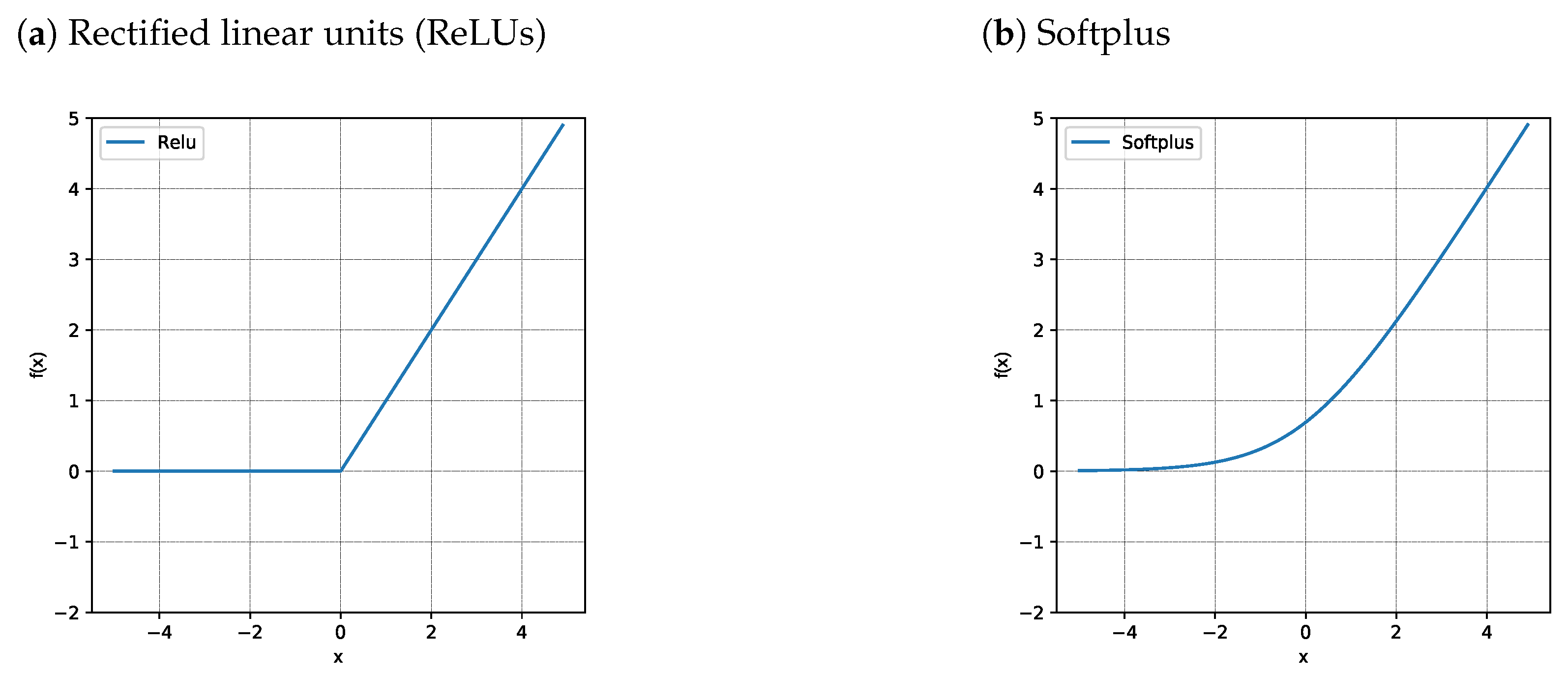
| Hidden layer activation function | ReLU |
| Output layer activation function | Softplus |
| Optimizer | Adam |
| Batch size | 64 |
| Epochs | 20 |
| Network Type | MSE | RMSE | |
|---|---|---|---|
| ANN | 1.67 × 10⁻⁶ | 0.001291 | 0.999948 |
| Bagging Ensemble | 1.23 × 10⁻⁷ | 0.000350 | 0.999996 |
| Metric | Analytical | ANN | Bagging Ensemble |
|---|---|---|---|
| Min price | R1.32 | R3.17 | R1.61 |
| Max price | R22,219.81 | R22,221.17 | R22,216.90 |
| Min absolute error | N/A | R0.00 | R0.00 |
| Max absolute error | N/A | R148.30 | R47.62 |
| Network Type | MSE | RMSE | |
|---|---|---|---|
| ANN | 1.63 × 10⁻⁶ | 0.001276 | 0.999952 |
| Bagging Ensemble | 1.99 × 10⁻⁷ | 0.000446 | 0.999994 |
| Metric | Analytical | ANN | Bagging Ensemble |
|---|---|---|---|
| Min price | R1.32 | R6.65 | R3.40 |
| Max price | R23,553.12 | R23,479.49 | R23,543.68 |
| Min absolute error | N/A | R0.02 | R0.00 |
| Max absolute error | N/A | R194.81 | R63.68 |
| Parameter | Trade 1 | Trade 2 | Trade 3 |
|---|---|---|---|
| Trade type | Call | Call | Call |
| Spot price of the underlying asset | R51,564.09 | R51,564.09 | R51,564.09 |
| Strike | R42,716.80 | R53,396.00 | R64,075.20 |
| Time to maturity | 345 days | 345 days | 345 days |
| Implied volatility | 22.32% | 18.50% | 15.17% |
| Repurchase agreement rate | 7.00% | 7.00% | 7.00% |
| Funding rate | 8.50% | 8.50% | 8.50% |
| Parameter | Trade 1 | Trade 2 | Trade 3 |
|---|---|---|---|
| Trade type | Call | Call | Call |
| Spot price of the underlying asset | R51,564.09 | R51,564.09 | R51,564.09 |
| Strike | R42,716.80 | R53,396.00 | R64,075.20 |
| Time to maturity | 345 days | 345 days | 345 days |
| Implied volatility | 22.32% | 18.50% | 15.17% |
| Repurchase agreement rate | 7.00% | 7.00% | 7.00% |
| Collateral rate | 5.50% | 5.50% | 5.50% |
| Option | Monte Carlo | Bagging Ensemble |
|---|---|---|
| Zero Collateral: Trade 2 | 0.035036 | 2.421635 |
| Fully Collateralized: Trade 2 | 0.060940 | 1.670318 |
| Option | Monte Carlo | Bagging Ensemble |
|---|---|---|
| Zero Collateral | 353.856228 | 18.082844 |
| Fully Collateralized | 356.446953 | 17.612219 |
Publisher’s Note: MDPI stays neutral with regard to jurisdictional claims in published maps and institutional affiliations. |
© 2021 by the authors. Licensee MDPI, Basel, Switzerland. This article is an open access article distributed under the terms and conditions of the Creative Commons Attribution (CC BY) license (https://creativecommons.org/licenses/by/4.0/).
Share and Cite
du Plooy, R.; Venter, P.J. A Comparison of Artificial Neural Networks and Bootstrap Aggregating Ensembles in a Modern Financial Derivative Pricing Framework. J. Risk Financial Manag. 2021, 14, 254. https://doi.org/10.3390/jrfm14060254
du Plooy R, Venter PJ. A Comparison of Artificial Neural Networks and Bootstrap Aggregating Ensembles in a Modern Financial Derivative Pricing Framework. Journal of Risk and Financial Management. 2021; 14(6):254. https://doi.org/10.3390/jrfm14060254
Chicago/Turabian Styledu Plooy, Ryno, and Pierre J. Venter. 2021. "A Comparison of Artificial Neural Networks and Bootstrap Aggregating Ensembles in a Modern Financial Derivative Pricing Framework" Journal of Risk and Financial Management 14, no. 6: 254. https://doi.org/10.3390/jrfm14060254
APA Styledu Plooy, R., & Venter, P. J. (2021). A Comparison of Artificial Neural Networks and Bootstrap Aggregating Ensembles in a Modern Financial Derivative Pricing Framework. Journal of Risk and Financial Management, 14(6), 254. https://doi.org/10.3390/jrfm14060254