Abstract
The yield curve is an important tool to assess the economic progress of a country. In this study, we examine the strength of the relationship between term spread and economic activity, and between the components of the yield curve and economic activity in the G7 countries using monthly data on yield rates and seasonally adjusted data on the industrial production index (IPI). After matching the start and end date of the IPI with the yield rates, the data used and respective time period are as follows: Canada: March-1994 to December-2018, France: January-1999 to December-2018, Germany: October-2005 to December-2018, Italy: July-2009 to December-2018, Japan: July-1994 to January-2019, the UK: January-1994 to December-2018, and the US: February-1990 to January-2019. The results show positive associations between term spread and economic activity for Canada, France, Germany, Japan, the UK, and the US. For Italy, a negative association is noted. All three empirical factors could predict economic activity for France and Germany at the 12-month horizon only. For all other horizons, the factors’ ability to predict economic activity varies. We observe that by including additional macro-finance variables such as the current economic growth rate and the 3-month yield rate to capture the term structure level effects, the relationship between term spread and economic activity becomes stronger. This implies that the usefulness of yield curve and its decomposed components for the purpose of predicting economic activity should be cautiously modelled and employed for policy.
1. Introduction
The yield curve, also known as the term structure of interest rates, is the relationship between the yield rates and the different maturity terms of specific type of assets such as government bonds. The yield curve plays an important role in pricing financial assets, conducting monetary policy, managing financial risk, and portfolio allocation. However, since Harvey (1988) and Estrella et al. (1991), a large amount of empirical literature has documented the leading indicator property of the slope of the yield curve and established it as an important tool for assessing and predicting the economic progress of a country. The shape of the yield curve indicates the view of the market participants regarding economic activity (Sowmya et al. 2016; Vieira et al. 2017). The term structure relationship can be best seen by examining yields on government bonds because they are similar in terms of having almost zero default risk, tax treatment, and marketability. It is important to note that the shape of the yield curve does not remain constant over time. Thus, as the general level of interest rises or falls, yield curves correspondingly shift up or down and have different slopes. The term spread, which is the difference between long-term rate and the short-term rate, is used to predict economic activity (Prasanna and Sowmya 2017). Examining the relationship between the term spread and economic activity, and subsequently the ability of the yield curve to predict economic activity, is of interest to policy makers, financial planners, and investors.
Financial institutions, such as banks and other credit institutions, consider the shape of the yield curve an important tool in financial management. Financial intermediaries borrow funds in financial markets from surplus spending units and lend them to businesses and consumers. An upward sloping yield curve is generally favorable for banks because they borrow most of their funds in the short-term (liability) and lend the funds (assets) at longer maturities. A steeper upward sloping yield curve indicates a wider spread between the borrowing and lending rates, and subsequently an increased profit for the financial intermediaries. Periods of economic expansions are characterized by low interest rates in the initial periods and the yield curve is upward sloping. However, when the yield curve begins to flatten out or to slope downward, it signals the inception of economic contraction, and different portfolio management strategies are invoked because the short-term rates tend to be at least as high as the long-term rates. Thus, as the yield curve becomes flatter, financial institutions will avoid locking in relatively expensive sources of funds for a longer period of time by shortening the maturity of liabilities and lengthening the maturity of assets (loans); the latter strategy is taken to lock in relatively high borrowing rates.
From a macroeconomic perspective, the short-term interest rate is a policy instrument under the direct control of the central bank, which is adjusted to achieve economic stabilization goals. From a finance perspective, the short-term rate is a fundamental building block for yields of other maturities measured as risk-adjusted averages of expected future short rates. Thus, a macro-finance perspective provides the most comprehensive understanding of the term structure of interest rates (Diebold et al. 2005). Several studies mainly use the term spread as independent variable to estimate the growth of output; the latter is measured by variables such as the GDP growth rate, the industrial production index, or the composite concurrent index. The analysis has been extended by decomposing the term structure of interest rate into three components: level, slope, and curvature (Chinn and Kucko 2015; Argyropoulos and Tzavalis 2016; Boukhatem and Sekouhi 2017). The decomposed factors are important in that the level factor captures the market participants’ expectations of the inflation. The slope factor captures the business cycle conditions and thus can be influenced by the monetary policies of the central banks, and the curvature factor captures the movements in the short-term rates as a result of the actions of the central bank.
In this study, we examine the relationship between the term spread and output growth with reference to the G7 countries (Canada, France, Germany, Italy, Japan, the United Kingdom, and the United States). To this end, we analyze both the term spread and its empirical components viz. future economic activity of the G7 countries, in terms of 1-month, 3-month, 6-month, 12-month, and 24-month horizons. Additionally, the analysis is extended to additional independent variables—the 3-month (short-term) interest rate and current economic growth—for these horizons. The remainder of the paper is organized as follows. In Section 2, we provide a brief literature review on the term structure of interest rates. In Section 3, we present the models and method used. In Section 4, we present the results and analysis. Section 5 discusses the key findings and Section 6 concludes.
2. Literature
The theories that explain the shape of the yield curve include expectations, liquidity premium, and segmentation theories. The expectation theory holds that the shape of the yield curve is determined by the investors’ expectations of future interest rate movements (Cox et al. 1981). The changes in the expectations change the shape of the yield curve. The theory assumes investors maximize profits and are indifferent in their preference between holding long-term and short-term securities. In this regard, they are indifferent toward interest rate risks. Thus, when investors expect the short-term interest rates to rise in the future, this is captured in the upward sloping yield curve and indicates economic expansion. Similarly, when there are expectations that short-term interest rates will decrease, the yield curve is downward sloping. This indicates a slowdown of economic activity or recession ahead. A flat yield curve indicates the view that the economy is in a mid-cycle period, that is, a possible transition that can move in the direction of expansion or contraction.
Based on the liquidity premium theory, investors prefer short-term bonds to long-term bonds, and therefore are willing to hold the latter at a premium, thus giving a positively-sloped yield curve. This is because long-term bonds are associated with price risk and are relatively illiquid. The market segmentation theory holds that investors have strong preferences for certain maturities over others, and therefore investors who prefer short-term bonds define the shape of the yield curve for short-term bonds, and those who demand intermediate or long-term bonds determine the yield curve for the intermediate and long-term bonds (Culbertson 1957).
Expectations theory is often used to explain the shape of the yield curve and the market participants’ view regarding economic fundamentals. The theory is often invoked to explain the process by which the term structure of interest rate influences economic activity (Plakandaras et al. 2017; Dery and Serletis 2019). The theory assumes that the expected excess return on long-term bonds over short-term bonds remains fixed over time. Additionally, the return is dependent upon the maturity of the bonds. The long-term rates are determined by expectations of the future short-term interest rates. Thus, the long-term yield is a weighted average of the expected future short-term yields plus a maturity-specific constant risk premium (Nelson and Siegel 1987). The short-term interest rate can influence inflation, real consumption, real interest, and output growth (Argyropoulos and Tzavalis 2018). The short-term interest rate directly depends on the monetary policy actions of the central bank, and the bond market participants’ expectation of the prospective short-term real interest rates, inflation, and risk premium determines the long-term interest rates (Morell 2018).
The information implied by the term structure carries important practical implications (Duffee 2002, 2011) for investors, financial institutions, and policy planners, therefore the behavior of the yield curve is of interest to them. It must be noted that the central bank sets the short-term interest rate based on the inflation in the economy. Since the short-term interest rate affects long-term rates (Orphanides and Wei 2012), the central bank is able to influence the long-term rates via the short-term rates, and hence the inflation rate and economic activity.
The literature in general confirms expectations theory viz. the term structure of interest rates; that is, an increase in the long-term interest rate relative to the short-term rate is associated with an increase in real economic activity for a number of periods, in terms of quarters, months, or years ahead. Moreover, the term structure of interest rate is noted to vary over the business cycle. The short-term interest rate is lower during recessions. This is because the central bank reduces the policy indicator rate to improve economic growth. The long-term rates are higher than the short-term rates because of the expectation that the central bank will increase the short-term rates in the future given the possibility of high growth and a subsequent inflationary pressure. This results in a positive slope of the yield curve (term spread) in a recession (Hännikäinen 2017). However, in the state of high economic growth or inflationary pressures, which signals an overheating economy, the central bank may increase the short-term interest rate. This will slow down real economic activity. Such policy measures will also increase the long-term interest rates because the longer-term securities are not as liquid as the short-term ones, and so the long-term bondholders will require higher rates to compensate for holding relatively illiquid financial assets. If it is expected that the central bank will reduce interest rates in the future because of the expectation of a decline in economic activity or low inflation, then the short-term rate can increase more than the long-term rates. This will be reflected by the yield curve, as it will either flatten or invert.
An alternative explanation for the positive slope of the term spread is that an increase in short-term rates will increase the cost of funding. This will affect investment and hence lower the long-edge of the curve. Moreover, the demand for savings will increase due to precautionary motives; the latter arising from expectations of future recessions. This can result in the decline of future economic activity and thus flatten or invert the yield curve (Argyropoulos and Tzavalis 2016). On the other hand, a decrease in the short-term rate will result in a positive term spread because the demand for long-term bonds will increase relative to the demand for short-term bonds, thus showing a positive slope of the yield curve.
In one of the earliest studies, Kessel (1965) notes that the term spread, long-term interest rate minus the short-term interest rate, moved with business cycles. In other words, the gap between short-term and long-term interest rate became narrower before economic recession and wider preceding an economic expansion. Recent studies have examined the relationship between the term structure of interest rates or the yield curve and major economic fundamentals, such as growth in output, inflation, investment, consumption, the monetary policy stance of central banks, and other macro-finance variables (Hännikäinen 2017; Gupta et al. 2020).
Consistent with the observations of Stock and Watson (2004), D’Agostino et al. (2006) note that in the mid-1980s, the yield curve’s predictive ability declined. Their explanation coincides with Bordo and Haubrich (2008a, 2008b) and Giacomini and Rossi (2006) that the decline in the predictive ability of the yield curve was mainly due to the presence of the stability of the output growth and other macroeconomic indicators.
Chinn and Kucko (2015) consider eight countries in their analysis (Canada, France, Germany, Italy, Japan, Sweden, the United Kingdom, and the United States) and monthly data from 1970 to 2013. To measure economic activity, they use the industrial production index. The term spread is computed as the 10-year government bond rate minus the 3-month bond rates. They note that the coefficient of the term spread is positive and statistically significant: Canada (1.81), France (1.22), Germany (1.52), Italy (0.85), Japan (1.23), The Netherlands (1.03), Sweden (0.99), the UK (0.69), and the US (1.14). Additionally, they note the yield spread could only predict the recessions correctly for the United States, Germany, and Canada, but not for Japan and Italy.
However, it is argued that using only a single spread factor can obscure the information content of the yield curve (Argyropoulos and Tzavalis 2016). The advantages of using the decomposed factors of the yield curve are that they are popular among scholars and central banks; that they are heavily used to estimate and predict economic activity, inflation, consumption, and monetary policy stance, among other things; that they make the model parsimonious and easy to estimate; that they have better forecasting results across bond maturities (Argyropoulos and Tzavalis 2016); and that the model can capture time-series variations in yields with only one or two factors. The level factor captures the market participants’ view regarding the medium-term inflation targets (Rudebusch and Wu 2008). The slope factor reflects future business cycle conditions. Noting the expectations theory of term structure of interest rates, Piazzesi (2005) highlights that the slope of the yield curve can be influenced by the monetary policy shocks which come because of changes in the short-term rates triggered by the central bank when they exercise their monetary policy tools. The curvature factor captures the movements in the short-term rate and hence the monetary policy actions of the central banks (Bekaert et al. 2010).
Argyropoulos and Tzavalis (2016) use monthly data on zero-coupon interest rates over the period 1987:05–2009:05, with maturity intervals from 3 months to 120 months and examine four developed economies: Canada, Germany, the US, and the UK. The term spread is defined as the difference between the 5-year (60-month) and the 3-month zero-coupon interest rates. The study notes that term spread has a positive and statistically significant association with the future growth rate for all four countries over 3, 6, 12, and 24-month horizons, and the results remain significant for Canada, the US, and the UK when 3-month interest rate and the current growth rate are added as additional independent variables. Additionally, it was noted that the slope factor could predict economic activity for the last five years, and that the curvature factor could predict economic activity over the short term.
Møller (2014) uses the quarterly dataset of US Treasury bonds with maturities of 1, 3, and 5 years and seasonally adjusted quarterly data on real GDP over the period 1953:Q2–2011:Q4, in addition to the Fama and Bliss (1987) zero-coupon bond yields. The term spread is defined as the difference between the 5-year and the 1-year Treasury bond rates, and the curvature factor as the intermediate yield rates minus the average of the short-term yield and long-term yields. The study notes that the curvature consistently outperforms the yield spread for the majority of 30 years, and hence it has a relatively superior predictive power to forecast the growth of GDP. The study also notes that once the curvature factor is included in the model, the spread factor tends to be statistically insignificant.
Hännikäinen (2017) uses the monthly dataset of US Treasury security yields over the period 1961:6–2015:4 to examine the predictive power of term structure of interest rates to forecast economic activity. In this study, the latent versions of level, slope, and curvature are extracted using the dynamic NS model (Diebold and Li 2006). In regards to the empirical version of the respective factors, the level factor was denoted by the 10-year yield rates (long-term rate), the slope factor was calculated as 10-year rates minus the 3-month rates (long-term minus the short-term rates), and the curvature was computed as two times the 2-year yield less the sum of the 3-month and 10-year rates. The study notes that the correlations between the latent and the empirical computed components were 0.98, 0.98, and 0.99 for the level, the slope, and the curvature factors, respectively. Their analysis showed that slope factor can predict economic activity, but the level and curvature factors were not the leading indicators. Furthermore, the yield curve’s ability to predict economic activity varied over time, a finding which is consistent with various studies (Mody and Taylor 2003; Levant and Ma 2017).
The declining ability of the yield curve to predict economy growth was re-examined by Morell (2018) for the US economy. Morell uses a dynamic stochastic general equilibrium model proposed by Feroli (2004) because the method accounts for the structure of the economy and the functional form of the reaction function of the central bank. Morell examines whether the decline in the predictive ability of the terms spread can be attributed to the time-varying term premia (TVTP), the presence of which can obscure the information content of the term spread and thus invalidate the expectations hypothesis. From the results, it was noted that TVTP is not statistically significant and thus not a factor that could have weakened the reliability of the term spread as a leading indicator. Based on the counterfactual analysis, Morell notes that shocks to the marginal efficiency of investment are the major driver of the fluctuations in the term spread and explain much of the decline in the predictive power of the term spread.
Plakandaras et al. (2017) develop non-linear econometric and machine-learning models to examine the information content of the term spread for the US economy. Their findings suggest that when considering the entire out-of-sample period, all models outperform the random walk model. Furthermore, their study concludes that models based on term spread are not efficient in point forecasting US inflation, and that linear models should be preferred over the more complex nonlinear ones.
3. Materials and Methods
Our sample consists of the G7 countries (Canada, France, Germany, Italy, Japan, the United Kingdom, and the United States). The G7 is chosen as a sample because it comprises large economies in terms of gross domestic product (GDP) and population, and because the countries in the G7 have well-developed, robust, and similar financial markets in terms of sophistication and size (Chinn and Kucko 2015). Moreover, the economic fundamentals of the G7 countries are generally similar, making them highly integrated, and hence the economic progress of the G7 has a significant influence or spillover effects on other developed and emerging countries, which effectively shape the direction of the world economy (Shahzad et al. 2017; Ha 2020).
We compiled monthly data on the interest rates of government bonds for the G7 countries (Canada, France, Germany, Italy, Japan, the UK, and the USA), for 3-month, 12-month, 36-month, 60-month, and 120-month zero-coupon bond rates. The data on interest rates for Canada, France, Germany, Italy, Japan, and the UK was compiled from the Fusion Media (2019a, 2019b) database. The end-of-month data for the US government bond rates was extracted from the US Department of the Treasury (2019) database. Noting a strong correlation between 60-month and 120-month yield rates, we used the 3-month rate for the short-term rates and the 60-month (5-year) rate for the long-term rates (Argyropoulos and Tzavalis 2016).
Moreover, seasonally adjusted data for the industrial production index (IPI) at 2015 constant prices were drawn from the available OECD (2019a) database. As noted by Chinn and Kucko (2015), the IPI data are reliable, timely, and closely follow GDP. Therefore, after matching the start and end date of the IPI with the yield rates, the sample data for each country is as follows: Canada = 1994:03–2018:12, France = 1999:01–2018:12, Germany = 2005:10–2018:12, Italy = 2009:07–2018:12, Japan = 1994:07–2019:01, the UK = 1994:01–2018:12, and the US = 1990:02–2019:01. Using the respective samples, we calculated the k-month-ahead growth rates as a dependent variable.
The least squares regression method was used for estimation. In line with various studies (Chinn and Kucko 2015; Argyropoulos and Tzavalis 2016; Ha 2020), we used the heteroskedasticity and autocorrelation consistent covariance (HAC) adjusted standard errors (Newey and West 1987, http://www.eviews.com/help/helpintro.html#page/content%2FRegress2-Robust_Standard_Errors.html%23 (accessed on 2 April 2019)). In Appendix B, we present the link between long-term and short-term rates and the future economic activity, the formula for the term spread and its empirical components, and the model for estimations.
4. Results
4.1. Graphical Analysis of the Term Spreads in G7 Countries
The Figure 1, Figure 2, Figure 3, Figure 4, Figure 5, Figure 6 and Figure 7 show the periods of economic expansion and slowdown in the G7 countries. The term spread based on the 3-month and the 5-year bond rates (black solid line) and the 3-month and 10-year rates (blue solid line) move in the same directions and are positively correlated.
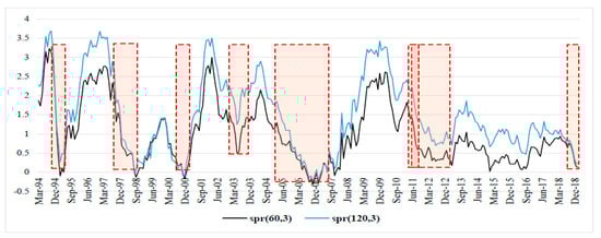
Figure 1.
Yield spread-Canada.
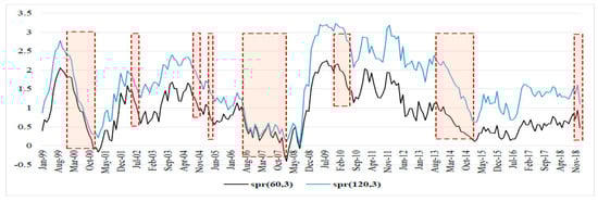
Figure 2.
Yield spread-France.
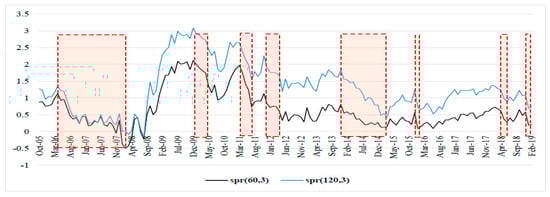
Figure 3.
Yield spread-Germany.
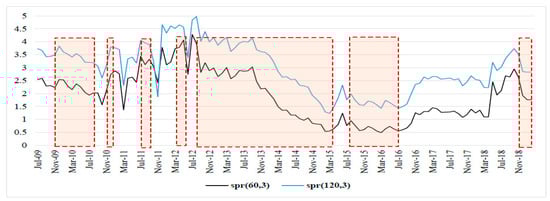
Figure 4.
Yield spread-Italy.
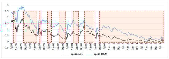
Figure 5.
Yield spread-Japan.
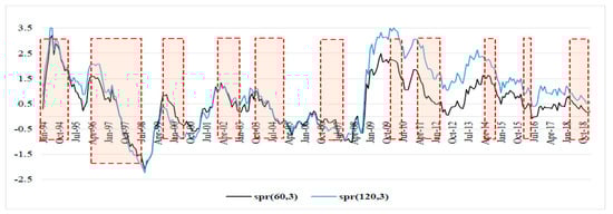
Figure 6.
Yield spread-UK.
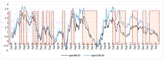
Figure 7.
Yield curve-US.
A common observation between all the countries, except for Italy because of missing data from earlier than 2009, is that they were affected by the 2007–2008 global financial crisis (GFC). The term spread started to decline at least 12 months before the onset of the GFC, and this is consistent for all countries (Figure 1, Figure 2, Figure 3, Figure 5, Figure 6 and Figure 7). Moreover, the term spread for the UK and the US started to decline from as early as 2004, thus signaling economic slowdown in the two economies much earlier than the other countries in the G7, and the effect of this later culminated into the GFC of 2007–2008.
In all the G7 countries, we note a general uniform decline in the term spread since 2010 at least, with few instances of increasing term spread, however, these were below the pre-2010 levels. Moreover, the term spread appears to be decreasing from mid-2018 for all the G7 countries. This signals a slowdown of economic activity in the G7 countries in periods leading up to 2019 (Roubini 2019).
4.2. Correlation Analysis
Table 1 shows the term spread correlations between G7 countries. Except for the pairs UK–Italy, UK-–Japan, and US–Italy, all the country pairs have generally positive and statistically significant correlations. The positive correlation coefficients are relatively strong for Germany–France (0.92), Italy–France (0.67), Germany–Canada (0.84), Germany–UK (0.78), Canada–US (0.70), UK–France (0.64), US–France (0.50), and UK–US (0.68). This can indicate that financial markets in these countries co-move relatively strongly. Moreover, there are no significant correlations between Italy–UK, Italy–US, Japan–UK and Japan–US.

Table 1.
Correlation matrix: spr(60,3).
4.3. Regression Results
Table A1 (Appendix A) provides the results of the estimation where the term spread is used as a single independent variable. The coefficient of the term spread is positive and significant for Canada and Germany at k = {1, 3, 6, 12, 24} month horizons, for France at k = {3, 6, 12, 24} month horizons, for Japan at k = {1, 3 6} month horizons, for the UK at k = {6, 12, 24} month horizons, and for the US at k = {12, 24} month horizons. These results imply a positive association between the term spread and the economic activity for respective k-month horizon. Except for Italy, where we noted a negative coefficient of the term spread, all the other G7 countries have a generally positive term spread, at least up to 12-month horizons. This implies that the yield curve has an upward sloping shape and hence the market participants’ views are in line with the expectations theory and the economic fundamentals. The results based on the marginal change (Table A3 in Appendix A) are generally consistent with the cumulative change results of Table A1.
For Italy (Table A1, Table A2 and Table A3), we note that the term spread has a negative association with the economic activity in all k-month horizons. This implies that a positive value of the spread () predicts a slowdown of the economic activity for Italy. The negative association is plausible when the increase in the long-term bond rate is only marginally higher than the short-term rates, and when there is a subsequent investors’ preference to hold long-term bonds instead of short-term bonds. This can be the case especially if the investors or market participants have a pessimistic outlook of the economy (FocusEconomics 2019).
Although there has been some evidence of a slow decline in the debt level of Italy, the share of debt of Italy held by non-residents is just about 33 percent (Zoli 2013; Kounis 2018). Two plausible explanations can be offered in the case of Italy. First, investors may prefer to hold long-term bonds if they expect that over the long-term. Thus, as the demand for long-term bond increases based on positive long-term expectations, the price of bond increases, and hence long-term yield rates will decrease. Second, there can be a greater preference for short-term bonds due to higher risks over the long-term. In this case, the demand for short-term bonds will increase, the prices will increase, and hence the short-term bond interest rates will decrease. Additionally, if the prices of the short-term bonds are above their par value, then the zero-coupon bond will have a negative interest rate. We note from the data that Italy’s long-term (5-year and 10-year) government bonds show a gradual decline in the yield rates since 2012, and the short-term rates have become negative since mid-2015, thus resulting in the widening of the term spread (see Figure 8 below).
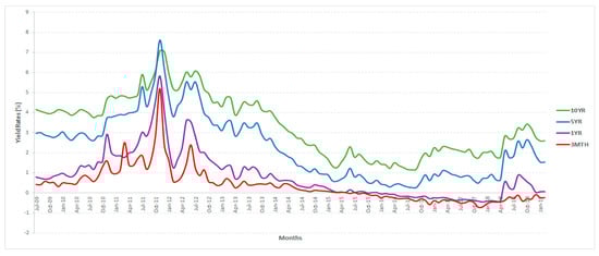
Figure 8.
Government bond data plot for Italy.
In Table A3, the results include the 3-month rate and the current period growth rate as additional independent variables. The 3-month rate captures the term structure’s level effects, and the captures the dynamics of economic growth on future economic activity (Dewachter et al. 2014). As noted from Table A3 and Table A4 (marginal change analysis), the coefficient of the term spread , is similar to the results obtained in Table A1 and Table A2 in terms of the signs and magnitudes for respective the k-month horizons. Moreover, by including and , we note that the coefficient of the term spread becomes statistically significant for additional k-month horizons; that is, at k = 12 for Japan, and k = {1, 3} for the UK and the US. Thus, not only do the augmented models retain the predictive power of term spread, they also improve the term spread’s ability to predict economic activity. The coefficients of 3-month rate and current period economic growth rate and , respectively, vary in terms of magnitude and level of significance. The results confirm that both the additional variables are important influencers of the economic activity of the G7 countries. For Canada, is negative at k = {3, 6, 12, 24}, and is positive at k = {1, 3, 6, 12} month horizons, although they are not significant within the 1–10 percent levels. For France, Germany, Italy, and Japan, is negative and significant at k = {12, 14}, k = {24}, k = {2, 6, 12, 24}, and at k = {1, 3, 6, 12}, respectively. In the UK and the US, generally is positive, but not statistically significant, for most of the k-month horizons, thus implying that the 3-month interest rate on its own does not contain (enough) information to predict economic activity. The negative (positive) coefficient of the 3-month bond rate implies that an increase (decrease) in the short-term rate slows down (speeds up) future economic activity.
The coefficient of the current economic growth rate varies among the G7 countries. For Canada, is generally positive but not significant, whereas for the US, it is positive and significant for all k-month horizons. This implies that the current economic growth of the US has a positive effect on its future economic activity. This is plausible if the market participants in general perceive that the US economy is heading in the right direction in terms of growth and development. For France and Italy, is negative and significant at k = {1, 24} and k = {3, 6, 12, 24}, respectively, whereas for the UK, is generally negative over the k-month horizons, however it is only significant at k = 1. A indicates that current period economic growth has a negative effect on future economic activity, and hence denotes a pessimistic outlook for market participants. In the case of Germany and Japan, is only significant at k = 24, thus indicating that current period economic growth affects economic activity over a long-term horizon. The results from the sub-sample (marginal change) estimations are presented in Table A4 (Appendix A) and they are consistent with the results presented in Table A2. Overall, the results indicate that the term spread has greater information content to predict future economic activity when additional variables such as the current growth and short-term rates are included in the model (Fendel et al. 2019).
Next, we estimate the relationship between the empirical components—level, slope, and curvature—as independent variables, and the economic activity of k-month horizons (see Table A5). The level factor is the 5-year (long-term) bond rate. The effects of vary for each country, both in terms of magnitude and horizons. A negative coefficient of implies that an increase in the 5-year bond rate will slow down economic activity over the k-month horizon. The coefficient is negative and significant for France at k = {3, 6, 12, 24} with {−1.07, −1.01, −0.97, −0.70}; for Germany at k = {12, 24} with {−2.40, −1.70}; for Italy at k = {6, 12} with {−1.25, −1.57}; and for Japan at k = {1, 3, 6, 12} with {−5.04, −6.30, −7.37, −7.05}. However, for Canada, the UK, and the US, is not significant over the k-month horizons, although using a sub-sample (k = 36, j = 24), is positive for the UK, {0.26}, and the US, {0.43}. Thus, the results indicate that the level factor’s ability to predict economic activity varies across the G7 countries and is evident in France, Germany, Italy, and Japan; but in the case of Canada, the UK, and the US, its ability to predict the economic activity has declined.
The coefficient of the slope factor, which is the difference between the short-term rate and the long-term rate (the opposite calculation of the term spread), is negative and significant for Canada at k = 1 and for the sub-sample (k = 36, j = 24); for France at k = {12, 24}; for Germany at k = {6, 12, 24} and for the sub-samples; for Japan at k = {1, 3, 6, 12} and the sub-sample (k = 36, j = 24); for the UK only for the sub sample (k = 36, j = 24); and the US at k = 24 and for the sub-sample (k = 36, j = 24). The results indicate that the slope factor’s ability to predict economic activity in the G7 countries varies across the countries and between k-month horizons. For Canada, France, and Germany, the slope predicts economic activity only for some k-month horizons, whereas for Japan, the slope factor predicts economic activity for all the k-month horizons. Although the coefficients of the slopes are negative for Italy and the UK at all horizons, they are not statistically significant. This implies that the slope factor does not contain sufficient information to predict economic activity for all the k-month horizons in the two countries.
The coefficient of the curvature factor for the G7 countries varies in terms of magnitudes, signs, and the statistical significance. The curvature factor captures the maximum (peak) and minimum (trough) of the yield curve. A positive coefficient implies a minimum, and a negative coefficient implies a maximum (in the sense of second order derivatives). Curvature is significant for Canada at k = 1 (), France at k = {1, 3, 6, 12} () and at the sub-sample at k = 36, j = 24; for Germany at k = {3, 6, 12} () and at the sub-sample at k = 36, j = 24; and for Italy at k = 24 () and the sub-sample at k = 24, j = 12. The results imply that in the case of Canada, Germany, and Italy, when the yield curve is at its minimum, future economic activity is expected to rise in the respective k-month horizons. However, for Japan, the UK, and the US, the curvature factor is not statistically significant at all k-month horizons, thus implying that for these countries, the peaks and troughs of the yield curve do not contain sufficient information to predict the future economic activity. Additionally, for France and Germany, at k = 12 month horizons, the level, slope, and curvature are significant. This implies that for these two countries, the empirical components of the yield curve are important considerations in predicting economic activity.
In regards the coefficient of the current period economic growth , it is significant and negative for France at k = {1, 24} month horizons, for Germany at k = 24 month horizon, Italy at k = {1, 3, 6, 12, 24} month horizons, Japan at k = 24 month horizon, and the UK at k = {1, 24} month horizons. However, for the US, is positive and significant at k = {6, 12, 24} month horizons, and for Canada, is not statistically significant at all k-month horizons. These results indicate that current period economic growth negatively influences the respective k-month forecasts for France, Germany, Italy, Japan, and the UK. Notably, at all k-month horizons for Italy. However, in the case of US, current period economic growth has a positive effect on future economic activity at least over k = {6, 12, 24} month horizons.
5. Discussion
From the different set of analyses presented, it is clear that the term spread and its empirical components have information content to predict economic activity. Moreover, the association between the term spread and economic activity becomes stronger when additional variables such as short-term interest rate and current economic growth are included in the model. Using the 3-month interest rate and the current period economic growth rate, we noted that the term spread’s ability to predict future economic activity improved over the k-month horizons.
Interestingly, we note a negative association between the term spread and the future economic activity for Italy, which to some extent can be attributed to an increase in the long-term bonds (debt) obtained at a relatively high interest rate (risk premium) in efforts to boost economic activity (Girardi 2019). Relatively high long-term bond rates on one hand and declining short-term rates on the other are not consistent with the theories that explain the yield curve, thus giving a signal that Italy’s economy could be experiencing some serious economic turbulences (Walker 2018). The average (2013–2018) net borrowing as a percent of GDP is 2.6 percent, and tax revenue as a percent of GDP is close to 42.6 percent (OECD 2019b, 2018, p. 3). Because there is less fiscal space to raise finance, given that Italy already has relatively high tax rates and government deficits, raising funds through long-term bonds becomes an option for Italy. As of mid-2015, the interest rates on 3-month, 1-year, and 3-year bonds were close to zero and in most part negative for the 3-month and 1-year bonds. Moreover, the interest rates on the long-term bonds (5-year and 10-year) have declined significantly from around 5% (early 2009) to around 2.5% (2019). The low rates do not incentivize to investors to hold bonds, and particularly short-term bonds with extremely low, and in some instances below zero, interest rates. This creates some divergence in terms of investors’ preferences to hold government bonds. In the case of Japan, government debts experienced growth, and this could create some turmoil in the financial markets (Krugman 2011; Sumner 2019). Although Japan is the most indebted developed country in the world, unlike Italy, which has a large share of government bonds held by non-residents, Japanese bonds are mostly held domestically. This gives Japan greater fiscal space to manage debt internally (Pham 2017). Furthermore, the declining trend of the term spread close to zero indicates some countries’ possible entrance into a liquidity trap, a situation where any further decrease in interest rate is not possible. Thus, to boost future economic activity, the role of fiscal coordination could become necessary.
6. Conclusions
The study set out to examine the ability of the term structure of interest rate to explain or predict economic activity. The term spread has a positive association with the k-month-ahead economic activity for Canada, France, Germany, Japan, the UK, and the USA, which is consistent with some earlier studies such as Chinn and Kucko (2015), and Argyropoulos and Tzavalis (2016). However, unlike Chinn and Kucko (2015), who note a positive association for Italy, we note that it has a negative association, even when additional factors were included in the estimation. In terms of the empirical components, we note that the effects of the level, slope, and curvature vary across the G7 countries and across the k-month horizons, which is consistent with Hännikäinen (2017) who examines the yield curves of US and Germany. Moreover, our results indicate that the statistical significance of all the variables, and particularly of the curvature factor, becomes stronger when the current period economic growth rate is included. Furthermore, the strength of the yield curve in terms of predicting economic activity is dependent on the inclusion of additional macro-finance variables. As noted, the relationship between term spread and economic activity becomes stronger (in a statistical sense) when additional variables such as short-term interest ratea and current economic growth are included in the model as independent variables (Boukhatem and Sekouhi 2017; Chinn and Kucko 2015; Fendel et al. 2019).
Some limitations of the study are in order. To decompose the term spread, we have used the empirical approach. A similar set of analyses can be based on latent components using the dynamic NS model. Additionally, the models presented in the study can be extended with additional macro-finance and structural variables to gain further insights. We have used the simple least squares method, but alternative approaches including non-linear techniques can be considered. We have only considered G7 countries, however, comparisons can be made with additional countries which have similar financial markets. Finally, we acknowledge that the predictive content of the term spread may not be policy independent. This implies that the problems of circularity may evolve when monetary authorities try systematically to respond to asset prices which themselves are based on the market’s anticipation of current and future policy actions. This does not invalidate the potential usefulness of the information incorporated in asset prices, but it indicates that economic policy instruments should be considered in the analysis. Therefore, the usefulness of yield curve and its decomposed components for the purpose of predicting economic activity should be cautiously modelled for policy purposes.
Author Contributions
Conceptualization, R.R.K.; methodology, R.R.K.; software, R.R.K.; validation, R.R.K. and P.J.S.; formal analysis, R.R.K., P.J.S. and H.T.T.V.; investigation, R.R.K.; resources, R.R.K.; data curation, R.R.K.; writing—original draft preparation, R.R.K.; writing—review and editing, P.J.S. and H.T.T.V.; visualization, R.R.K.; supervision, R.R.K. and P.J.S.; project administration, R.R.K. All authors have read and agreed to the published version of the manuscript.
Funding
This research received no external funding.
Institutional Review Board Statement
Not applicable.
Informed Consent Statement
Not applicable.
Data Availability Statement
Not applicable.
Acknowledgments
The authors thank the academic and managing editors, and the anonymous reviewers for their comments and suggestions. Peter Stauvermann thanks the Changwon National University for financially supporting his ongoing research work and collaboration. This research did not receive any funding. The usual disclaimer applies.
Conflicts of Interest
The authors declare no conflict of interest.
Appendix A
Table A1.
Economic activity and the term spread—cumulative change.
Table A1.
Economic activity and the term spread—cumulative change.
| Equation: | ||||||||||||||
| Horizon (k Months) | Canada | France | Germany | Italy | Japan | UK | US | |||||||
| , | , | , | , | , | , | , | ||||||||
| 1 | 2.94 *** (0.703) | 0.04, 297 | 0.54 † (0.756) | <0.01 †, 239 | 6.03 *** (1.964) | 0.02, 158 | −2.78 ** (1.076) | 0.02, 115 | 3.59 *,† (1.845) | <0.01 †, 259 | 0.68 (0.453) | <0.01 †, 299 | 0.63 (0.519) | <0.01 †, 347 |
| 3 | 2.65 *** (0.600) | 0.09, 295 | 2.32 ** (1.067) | 0.03, 237 | 6.65 *** (1.550) | 0.09, 156 | −2.02 *** (0.755) | 0.07, 113 | 2.59 ** (1.187) | <0.01 †, 292 | 0.87 (0.422) | 0.02, 297 | 0.61 (0.551) | 0.01, 345 |
| 6 | 2.26 *** (0.536) | 0.10, 292 | 2.40 ** (1.127) | 0.06, 234 | 7.26 *** (1.879) | 0.16, 153 | −2.10 *** (0.583) | 0.16, 110 | 2.02 * (1.152) | <0.01 †, 289 | 0.88 ** (0.417) | 0.05, 294 | 0.67 (0.520) | 0.01, 342 |
| 12 | 1.69 *** (0.533) | 0.10, 286 | 2.57 ** (1.121) | 0.13, 228 | 7.66 *** (2.122) | 0.32, 147 | −1.91 *** (0.426) | 0.23, 104 | 1.58 (1.206) | <0.01 †, 259 | 0.85 * (0.452) | 0.08, 288 | 0.94 * (0.463) | 0.03, 336 |
| 24 | 1.29 *** (0.486) | 0.12, 274 | 1.83 *** (0.668) | 0.15, 216 | 5.09 *** (1.219) | 0.37, 135 | −1.72 *** (0.221) | 0.41, 92 | -0.74 (0.736) | <0.01 †, 271 | 0.53 * (0.321) | 0.07, 276 | 1.40 *** (0.468) | 0.14, 324 |
Notes: We report HAC standard errors and covariance (Bartlett kernel, Newey–West fixed bandwidth = 5); ***, **, and * indicate the coefficient is statistically significant at a 1%, 5%, and 10% level, respectively. For Japan, at k = 1 and k = 12, I re-adjusted the end-date to 2016M01 to avoid negative . † For France, at k = 1, constant term was removed during estimation to avoid negative . Constant term is not significant in all cases, hence not reported to save space. is the adjusted coefficient of determination, and is the sample size. Source: Authors’ estimation. Source: Authors’ estimation.
Table A2.
Economic activity from the term spread—marginal change.
Table A2.
Economic activity from the term spread—marginal change.
| Equation: , for k = 24, j = 12 | ||||||||||||||
| Horizon | Canada | France | Germany | Italy | Japan | UK † | US | |||||||
| , | , | , | , | , | , | , | ||||||||
| k = 24, j = 12 | 2.16 (1.806) | 0.02, 273 | 2.89 (2.453) | 0.01, 216 | 7.33 (6.025) | 0.03, 135 | −4.17 *** (1.218) | 0.20, 92 | −7.76 (0.015) | 0.02, 271 | 0.31 (0.331) | 0.001, 276 | 6.197 *** (2.499) | 0.16, 324 |
| Notes: ***, **, and * indicate significance level at a 1%, 5%, and 10% level, respectively. † The start date of the sample was readjusted to 1996M01. | ||||||||||||||
| Equation:, for k = 36, j = 24 | ||||||||||||||
| Horizon | Canada | France | Germany† | Italy | Japan | UK | US | |||||||
| , | , | , | , | , | , | , | ||||||||
| k = 36, j = 24 | 2.16 ** (0.937) | 0.08, 261 | 0.65 (1.232) | <0.001 †, 198 | −0.96 (2.086) | 0.03, 101 | −2.75 *** (0.753) | 0.23, 80 | −4.61 * (2.368) | 0.07, 259 | 0.511 (0.485) | 0.01, 264 | 4.01 *** (0.9340) | 0.31, 312 |
| Notes: We report HAC standard errors and covariance (Bartlett kernel, Newey–West fixed bandwidth = 5); ***, **, and * indicate the coefficient is statistically significant at a 1%, 5% and 10% level, respectively. † Sample for Germany was re-adjusted to 2007M08-2019M02 to correct for negative . Constant term is not significant in all cases, hence not reported to save space. is the adjusted coefficient of determination, and is the sample size. Source: Authors’ estimation Source: Authors’ estimation. | ||||||||||||||
Table A3.
Economic activity from the term spread, short rate, and growth rate—cumulative change.
Table A3.
Economic activity from the term spread, short rate, and growth rate—cumulative change.
| Equation: | ||||||||||||
| Horizon (k Months) | Canada | France | Germany | |||||||||
| , | , | , | ||||||||||
| 1 | 2.92 *** (0.765) | 0.04 (0.365) | <0.01 (0.096) | 0.03, 296 | 1.77 (1.404) | −0.32 (0.474) | −0.35 *** (0.097) | 0.11, 238 | 6.14 *** (2.287) | −0.20 (1.105) | −0.05 (0.208) | 0.01, 157 |
| 3 | 2.45 *** (0.596) | −0.10 (0.301) | 0.07 (0.072) | 0.10, 294 | 2.18 ** (0.984) | −0.43 (0.406) | −0.05 (0.058) | 0.04, 236 | 6.12 *** (1.377) | −0.59 (1.129) | 0.11 (0.127) | 0.12, 155 |
| 6 | 2.10 *** (0.517) | −0.16 (0.267) | 0.06 (0.054) | 0.11, 291 | 2.14 ** (0.948) | −0.62 (0.428) | −0.02 (0.031) | 0.09, 233 | 6.55 *** (1.367) | −1.11 (1.316) | 0.06 (0.059) | 0.20, 152 |
| 12 | 1.63 *** (0.520) | −0.20 (0.224) | 0.01 (0.027) | 0.10, 285 | 2.24 ** (0.936) | −0.67 ** (0.330) | −0.01 (0.013) | 0.19, 227 | 6.87 *** (1.533) | −1.41 (0.953) | 0.01 (0.021) | 0.40, 146 |
| 24 | 1.28 *** (0.466) | −0.19 (0.197) | −0.01 (0.014) | 0.12, 273 | 1.43 *** (0.510) | −0.65 *** (0.204) | −0.02 *** (0.006) | 0.30, 215 | 4.31 *** (0.997) | −1.42 *** (0.382) | −0.04 *** (0.013) | 0.59, 134 |
| Horizon (k Months) | Italy | Japan | UK | |||||||||
| , | , | , | ||||||||||
| 1 | −3.56 ** (1.460) | 0.60 (1.220) | −0.38 *** (0.062) | 0.15, 114 | 5.71 *** (1.845) | −5.66 ** (2.908) | 0.09 (0.164) | 0.01, 293 | 0.97 * (0.531) | 0.20 (0.189) | −0.19 ** (0.96) | 0.03, 298 |
| 3 | −1.44 (0.931) | −1.71 * (0.921) | −0.13 *** (0.029) | 0.18, 112 | 6.12 *** (1.972) | −6.53 * (3.485) | 0.05 (0.113) | 0.02, 291 | 1.04 ** (0.442) | 0.13 (0.141) | −0.06 (0.054) | 0.03, 296 |
| 6 | −1.45 ** (0.650) | −1.53 ** (0.672) | −0.05 *** (0.016) | 0.24, 109 | 6.11 *** (2.200) | −7.42 * (4.11) | 0.04 (0.055) | 0.05, 288 | 0.95 ** (0.403) | 0.05 (0.119) | −0.02 (0.031) | 0.05, 293 |
| 12 | −1.03 ** (0.440) | −1.86 *** (0.551) | −0.03 ** (0.013) | 0.38, 103 | 4.89 ** (2.199) | −6.77 * (3.852) | −0.02 (0.027) | 0.07, 282 | 0.86 ** (0.430) | 0.002 (0.094) | −0.007 (0.017) | 0.07, 287 |
| 24 | −1.06 *** (0.294) | −1.54 ** (0.628) | −0.03 *** (0.008) | 0.60, 91 | 0.51 (1.010) | −2.18 (2.251) | −0.03 * (0.013) | 0.04, 270 | 0.52 * (0.297) | −0.02 (0.088) | −0.01 (0.006) | 0.07, 275 |
| Horizon (k Months) | US | |||||||||||
| , | ||||||||||||
| 1 | 0.93 ** (0.380) | 0.36 * (0.212) | 0.22 ** (0.093) | 0.06, 346 | ||||||||
| 3 | 0.79 ** (0.398) | 0.27 (0.188) | 0.26 *** (0.067) | 0.16, 344 | ||||||||
| 6 | 0.77 ** (0.401) | 0.20 (0.178) | 0.24 *** (0.064) | 0.18, 341 | ||||||||
| 12 | 1.01 *** (0.417) | 0.21 (0.154) | 0.18 *** (0.046) | 0.13, 335 | ||||||||
| 24 | 1.67 *** (0.466) | 0.27 ** (0.127) | 0.05 * (0.024) | 0.19, 323 | ||||||||
Notes: We report HAC standard errors and covariance (Bartlett kernel, Newey–West fixed bandwidth = 5); ***, **, and * indicate the coefficient is statistically significant at a 1%, 5% and 10% level, respectively. is the adjusted coefficient of determination, and is the sample size. Source: Authors’ estimation.
Table A4.
Economic activity and term spread, short rate, and growth rate—marginal change.
Table A4.
Economic activity and term spread, short rate, and growth rate—marginal change.
| Equation: , for k = 24, j = 12 | ||||||||||||
| Horizon (k Months) | Canada | France | Germany | |||||||||
| , | , | , | ||||||||||
| k = 24, j = 12 | 2.09 (1.696) | −0.20 (0.286) | −0.02 (0.024) | 0.02, 273 | 2.48 (2.209) | −0.66 * (0.393) | −0.03 ** (0.012) | 0.08, 215 | 4.79 (5.255) | −1.32 (1.292) | −0.09 *** (0.033) | 0.13, 134 |
| Horizon (k Months) | Italy | Japan | UK | |||||||||
| , | , N | , | ||||||||||
| k = 24, j = 12 | −3.55 ** (1.588) | −0.43 (0.837) | −0.01 (0.015) | 0.19, 91 | −12.86 * (6.796) | 2.78 (2.903) | −0.03 * (0.019) | 0.03, 270 | −0.06 (0.274) | −0.09 (0.135) | −0.02 (0.014) | <0.01, 275 |
| Horizon (k Months) | US | |||||||||||
| , | ||||||||||||
| k = 24, j = 12 | 6.42 *** (2.444) | 0.05 (0.177) | −0.06 ** (0.026) | 0.17, 323 | ||||||||
| Equation:, for k = 36, j = 24 | ||||||||||||
| Horizon (k Months) | Canada | France | Germany | |||||||||
| , | , N | , | ||||||||||
| k = 36, j = 24 | 2.17 ** (0.914) | −0.05 (0.190) | −0.01 (0.017) | 0.08, 261 | 0.01 (1.017) | −0.38 * (0.204) | −0.02 ** (0.008) | 0.04, 203 | −1.43 (2.377) | −0.72 (0.781) | −0.06 *** (0.023) | 0.09, 122 |
| Horizon (k Months) | Italy | Japan | UK | |||||||||
| , N | , N | , | ||||||||||
| k = 36, j = 24 | −2.37 ** (0.945) | −0.40 (0.488) | −0.01 (0.011) | 0.22, 79 | −9.33 *** (2.981) | 3.94 ** (1.782) | −0.02 ** (0.008) | 0.15, 258 | 0.46 (0.475) | −0.02 (0.088) | −0.01 (0.007) | 0.01, 263 |
| Horizon (k Months) | US | |||||||||||
| , | ||||||||||||
| k =36, j = 24 | 4.54 *** (0.908) | 0.29 ** (0.124) | −0.04 *** (0.018) | 0.35, 311 | ||||||||
Notes: We report HAC standard errors and covariance (Bartlett kernel, Newey–West fixed bandwidth = 5), ***, **, and * indicate the coefficient is statistically significant at a 1%, 5% and 10% level, respectively. is the adjusted coefficient of determination, and is the sample size. Source: Authors’ estimation.
Table A5.
Economic activity, levels, slope, curvature, and growth.
Table A5.
Economic activity, levels, slope, curvature, and growth.
| Equation: | ||||||||||||||||
| Horizon (k Months) | Canada | France | Germany | |||||||||||||
| , | , | , | ||||||||||||||
| 1 | −0.41 (0.379) | −0.08 (1.296) | 6.04 *** (1.971) | −0.02 (0.098) | 0.05, 296 | −0.99 (0.626) | 0.43 (1.917) | 7.49 ** (3.574) | −0.36 *** (0.092) | 0.12, 238 | −1.49 (1.749) | −1.64 (4.709) | 16.2 (11.34) | −0.06 (0.196) | 0.03, 157 | |
| 3 | −0.29 (0.303) | −1.33 (1.13) | 2.60 * (1.526) | 0.07 (0.072) | 0.10, 294 | −1.07 ** (0.522) | −0.26 (1.126) | 6.97 *** (2.255) | −0.06 (0.053) | 0.10, 236 | −1.76 (1.539) | −2.48 (2.834) | 14.6 * (7.906) | 0.10 (0.115) | 0.17, 155 | |
| 6 | −0.27 (0.262) | −1.54 (1.089) | 1.54 (1.460) | 0.05 (0.053) | 0.12, 291 | −1.01 ** (0.488) | −1.32 (1.172) | 4.30 ** (1.705) | −0.02 (0.029) | 0.13, 233 | −1.94 (1.453) | −4.69 * (2.444) | 10.2 * (5.391) | 0.05 (0.052) | 0.24, 152 | |
| 12 | −0.25 (0.231) | −1.59 (1.004) | 0.54 (1.254) | 0.01 (0.027) | 0.10, 285 | −0.97 ** (0.382) | −1.87 * (1.050) | 3.10 ** (1.397) | −0.02 (0.013) | 0.23, 227 | −2.40 *** (0.848) | −4.75 ** (2.102) | 12.2 *** (3.917) | 0.01 (0.019) | 0.50, 146 | |
| 24 | −0.18 (0.218) | −1.49 * (0.879) | −0.05 (1.021) | −0.01 (0.014) | 0.12, 273 | −0.70 *** (0.196) | −1.90 ** (0.783) | 0.52 (0.909) | −0.02 *** (0.006) | 0.30, 215 | −1.70 *** (0.289) | −4.78 *** (1.232) | 3.24 (2.111) | −0.04 *** (0.014) | 0.60, 134 | |
| 24,12 | −0.18 (0.298) | −1.27 (1.198) | −0.40 (1.501) | −0.02 (0.024) | 0.03, 273 | −0.41 (0.278) | −1.97 (1.408) | −2.13 (1.508) | −0.03 ** (0.012) | 0.09, 215 | −0.80 (1.220) | −4.98 * (2.738) | −6.22 (4.653) | −0.09 *** (0.030) | 0.16, 134 | |
| 36,24 | 0.06 (0.215) | −1.94 *** (0.674) | −1.19 (0.891) | −0.01 (0.017) | 0.12, 261 | 0.03 (0.209) | −1.31 (0.883) | −3.62 ** (1.433) | −0.01 (0.008) | 0.17, 203 | 0.29 (0.747) | −2.76 * (1.585) | −10.0 *** (3.468) | −0.05 *** (0.018) | 0.27, 122 | |
| Horizon (k Months) | Italy | Japan | UK | |||||||||||||
| , | , | , | ||||||||||||||
| 1 | 1.27 (1.510) | 3.16 (3.149) | −2.73 (4.422) | −0.37 *** (0.063) | 0.14, 114 | −5.04 * (2.837) | −11.80 ** (4.572) | −7.65 (7.862) | 0.09 (0.163) | 0.01, 293 | 0.04 (0.318) | −0.18 (1.204) | 1.25 (2.143) | −0.19 * (0.095) | 0.03, 298 | |
| 3 | −1.61 (1.065) | −0.43 (1.861) | −0.42 (2.162) | −0.13 *** (0.030) | 0.17, 112 | −6.30 ** (3.099) | −12.79 ** (5.462) | −2.70 (8.159) | 0.05 (0.113) | 0.02, 291 | −0.002 (0.253) | −0.43 (0.810) | 1.02 (1.602) | −0.06 (0.053) | 0.03, 296 | |
| 6 | −1.25 * (0.760) | −0.47 (1.411) | −1.11 (1.650) | −0.05 *** (0.018) | 0.24, 109 | −7.37 ** (−3.692) | −13.56 ** (6.298) | −0.56 (7.237) | 0.04 (0.055) | 0.05, 288 | −0.04 (0.187) | −0.56 (0.603) | 0.70 (1.039) | −0.02 (0.031) | 0.05, 293 | |
| 12 | −1.57 *** (0.581) | −1.17 (1.103) | −1.08 (1.150) | −0.03 ** (0.013) | 0.38, 103 | −7.05 * (3.836) | −11.47 ** (5.759) | 3.24 (4.740) | −0.02 (0.026) | 0.07, 282 | −0.17 (0.180) | −0.23 (0.491) | 1.32 (1.066) | −0.01 (0.016) | 0.09, 287 | |
| 24 | −1.11 * (0.685) | −1.06 (0.958) | −1.72 ** (0.689) | −0.02 *** (0.007) | 0.64, 91 | −1.90 (2.178) | −2.88 (3.112) | −2.98 (3.406) | −0.03 * (0.014) | 0.05, 270 | −0.03 (0.140) | −0.50 (0.387) | 0.07 (0.682) | −0.01 * (0.006) | 0.06, 275 | |
| 24, 12 | −0.08 (0.855) | −0.20 (1.330) | −2.13 * (1.129) | −0.02 (0.014) | 0.21, 91 | 3.24 (2.602) | 5.76 (4.652) | −9.17 (5.982) | −0.03 * (0.020) | 0.06, 270 | 0.09 (0.149) | −0.75 (0.605) | −1.14 (0.853) | −0.02 (0.013) | 0.01, 275 | |
| 36, 24 | −0.35 (0.555) | −0.43 (1.017) | −1.35 (1.129) | −0.01 (0.012) | 0.16, 79 | 3.84 ** (1.872) | 6.93 *** (2.544) | −9.51 * (4.999) | −0.02 ** (0.008) | 0.24, 258 | 0.26 ** (0.118) | −1.14 ** (0.498) | −1.70 ** (0.659) | −0.01 * (0.07) | 0.09, 263 | |
| Horizon (k Months) | US | |||||||||||||||
| , | ||||||||||||||||
| 1 | 0.16 (0.232) | 0.09 (0.562) | 1.78 (1.197) | 0.21 (0.106) | 0.06, 346 | |||||||||||
| 3 | 0.10 (0.255) | 0.05 (0.552) | 1.54 (1.160) | 0.26 (0.070) | 0.16, 344 | |||||||||||
| 6 | 0.04 (0.255) | −0.02 (0.536) | 1.15 (1.144) | 0.24 *** (0.073) | 0.18, 341 | |||||||||||
| 12 | 0.06 (0.234) | −0.36 (0.577) | 1.35 (1.215) | 0.15 *** (0.042) | 0.13, 335 | |||||||||||
| 24 | 0.114 (0.211) | −0.91 * (0.539) | 1.27 (1.161) | 0.04 ** (0.019) | 0.20, 323 | |||||||||||
| 24, 12 | 0.093 (0.302) | −1.29 (0.947) | 1.51 (1.864) | −0.06 ** (0.026) | 0.17, 323 | |||||||||||
| 36, 24 | 0.43 ** (0.215) | −2.21 ** (0.887) | −0.19 (1.172) | −0.04 ** (0.021) | 0.38, 311 | |||||||||||
Notes: We report the HAC standard errors and covariance (Bartlett kernel, Newey–West fixed bandwidth = 6); ***, **, and * indicate the coefficient is statistically significant at a 1%, 5% and 10% level, respectively. The 3-month rate was excluded from the country-specific regression estimation due to singular matrix (perfect collinearity) problems. is the adjusted coefficient of determination, and is the sample size. Source: Authors’ estimation.
Appendix B
The link between term spread and future economic activity can be expressed as follows:
where is the difference between output at time t + j and t. The term spread is the difference between long-term and short-term yields, in Equation (A1). For the dependent variable, we use the cumulative annualized economic values of the level of industrial production index computed as:
where k denotes the forecasting horizon in months, and is the level of industrial production index in month t + k. Thus, denotes the percentage change between the current month t and the future months t + k for IPI in each country i. Studies also use the annualized marginal percentage change in IPI from month t + k − j to month t + k, to examine the association between term spread and economic activity between two different periods. Thus, we define the economic activity as:
where j is the forecasting horizon in months.
The short-term and long-term rates are used to measure the slope of the yield curve or the spread. The long-term rate is the 60-month yield and the short-term rate is the 3-month yield rate . Hence, we define the term spread using 5-year (60-month) bond rate and 3-month bond rate as:
Similar to Hännikäinen (2017) and Afonso and Martins (2012), and drawing insights from Møller (2014), we decompose the term structure of interest rate into three components: level, slope, and curvature, as follows:
The association between the term structure of interest rate and the real economic activity (base equation) is expressed as follows:
where is a constant term, is the coefficient of each country’s (i) term spread at k horizon, and is the error term assumed to be normally distributed with mean zero and constant variance. We use the horizons months. To examine if the term spread can retain its predictive power using as a dependent variable, we estimate the following equation:
where is a constant for each country, i and months ahead and month horizon, and . Thus, (12) and (12); are the coefficient of the spread, and is the error term. Additionally, to review the robustness of the results, we estimate the following equations:
and
where is in included to capture the term structure level effects, and is the current economic growth rate defined as . The factor is added into the model to capture the current period’s growth on future economic activity. In the second set of analysis, we estimate the effect of level, slope, and curvature on the k-period-ahead economic activity. The basic specification is:
Similar to Equations (A9) and (A10), we estimate the following equations:
where , , and are level, slope, and curvature, respectively.
References
- Afonso, António, and Manuel M.F. Martins. 2012. Level, slope, curvature of the sovereign yield curve, and fiscal behaviour. Journal of Banking & Finance 36: 1789–807. [Google Scholar]
- Argyropoulos, Efthymios, and Elias Tzavalis. 2016. Forecasting economic activity from yield curve factors. The North American Journal of Economics and Finance 36: 293–311. [Google Scholar] [CrossRef]
- Argyropoulos, Efthymios, and Elias Tzavalis. 2018. The influence of real interest rates and risk premium effects on the ability of the nominal term structure to forecast inflation. The Quarterly Review of Economics and Finance. [Google Scholar] [CrossRef]
- Bekaert, Geert, Seonghoon Cho, and Antonio Moreno. 2010. New Keynesian macroeconomics and the term structure. Journal of Money, Credit and Banking 42: 33–62. [Google Scholar] [CrossRef]
- Bordo, Michael D., and Joseph G. Haubrich. 2008a. The yield curve as a predictor of growth: Long-run evidence, 1875–997. The Review of Economics and Statistics 90: 182–85. [Google Scholar] [CrossRef]
- Bordo, Michael D., and Joseph G. Haubrich. 2008b. Forecasting with the yield curve; level, slope, and output 1875–997. Economics Letters 99: 48–50. [Google Scholar] [CrossRef]
- Boukhatem, Jamel, and Hayfa Sekouhi. 2017. What does the bond yield curve tell us about Tunisian economic activity? Research in International Business and Finance 42: 295–303. [Google Scholar] [CrossRef]
- Chinn, Menzie, and Kavan Kucko. 2015. The predictive power of the yield curve across countries and time. International Finance 18: 129–56. [Google Scholar] [CrossRef]
- Cox, C. John, Jonathan E. Ingersoll, and Stephen A. Ross. 1981. A re-examination of traditional hypotheses about the term structure of interest rates. The Journal of Finance 36: 769–99. [Google Scholar] [CrossRef]
- Culbertson, John Mathew. 1957. The term structure of interest rates. The Quarterly Journal of Economics 71: 485–517. [Google Scholar] [CrossRef]
- D’Agostino, Antonello, Domenico Giannone, and Paolo Surico. 2006. (Un)predictability and Macroeconomic Stability. Working Paper Series No. 605. Frankfurt: European Central Bank, pp. 1–43. Available online: http://sdw.central.banktunnel.eu/pub/pdf/scpwps/ecbwp605.pdf (accessed on 1 February 2019).
- Dery, Cosmas, and Apostolos Serletis. 2019. Interest rates, money, and economic Activity. Macroeconomic Dynamics, 1–50. Available online: https://www.cambridge.org/core/journals/macroeconomic-dynamics/article/interest-rates-money-and-economic-activity/3B2A01D7DBBD9F6BDBFD9F91531E7AB5 (accessed on 12 January 2020). [CrossRef]
- Dewachter, Hans, Leonardo Iania, and Marco Lyrio. 2014. Information in the yield curve: A Macro-Finance approach. Journal of Applied Econometrics 29: 42–64. [Google Scholar] [CrossRef]
- Diebold, Francis X., and Canlin Li. 2006. Forecasting the term structure of government bond yields. Journal of Econometrics 130: 337–64. [Google Scholar] [CrossRef]
- Diebold, Francis X., Monika Piazzesi, and Glenn D. Rudebusch. 2005. Modeling bond yields in finance and macroeconomics. American Economic Review 95: 415–20. [Google Scholar] [CrossRef]
- Duffee, Gregory R. 2002. Term premia and interest rate forecasts in affine models. The Journal of Finance 57: 405–43. [Google Scholar] [CrossRef]
- Duffee, Gregory R. 2011. Information in (and not in) the term structure. The Review of Financial Studies 24: 2895–934. [Google Scholar] [CrossRef]
- Estrella, Arturo, and Gikas A. Hardouvelis. 1991. The term structure as a predictor of real economic activity. The Journal of Finance 46: 555–76. [Google Scholar] [CrossRef]
- Fama, Eugene F., and Robert R. Bliss. 1987. The information in long-maturity forward rates. The American Economic Review 77: 680–92. Available online: https://www.jstor.org/stable/1814539 (accessed on 2 February 2019).
- Fendel, Ralf, Nicola Mai, and Oliver Mohr. 2019. Predicting Recessions Using Term Spread at the Zero Lower Bound: The Case of the Euro Area. VOX CEPR Policyt Portal. January 17. Available online: https://voxeu.org/article/predicting-recessions-using-term-spread-zero-lower-bound (accessed on 8 April 2019).
- Feroli, Michael. 2004. Monetary policy and the information content of the yield spread. The BE Journal of Macroeconomics 4: 1–15. [Google Scholar] [CrossRef]
- FocusEconomics. 2019. Italy Economic Outlook. Barcelona: FocusEconomics. Available online: https://www.focus-economics.com/countries/italy (accessed on 15 April 2019).
- Fusion Media. 2019a. Investment.com. Available online: https://www.investing.com/rates-bonds/ (accessed on 2 February 2019).
- Fusion Media. 2019b. Investment.com. Available online: https://www.investing.com/about-us/ (accessed on 2 February 2019).
- Giacomini, Raffaella, and Barbara Rossi. 2006. How stable is the forecasting performance of the yield curve for output growth? Oxford Bulletin of Economics and Statistics 68: 783–95. [Google Scholar] [CrossRef]
- Girardi, Annalisa. 2019. Italy Falls Back into Recession as the World Fears Global Economic Slowdown. Forbes. Available online: https://www.forbes.com/sites/annalisagirardi/2019/02/01/italy-falls-back-into-recession-as-the-world-fears-global-economic-slowdown/#3e3b0590225f (accessed on 15 April 2019).
- Gupta, Rangan, Hylton Hollander, and Rudi Steinbach. 2020. Forecasting output growth using a DSGE-based decomposition of the South African yield curve. Empirical Economics 58: 351–78. [Google Scholar] [CrossRef]
- Ha, Jongrim. 2020. Nonlinear transmission of U.S. monetary policy shocks to international financial markets. International Finance. Available online: https://onlinelibrary.wiley.com/doi/abs/10.1111/infi.12371 (accessed on 30 March 2020). [CrossRef]
- Hännikäinen, Jari. 2017. When does the yield curve contain predictive power? Evidence from a data-rich environment. International Journal of Forecasting 33: 1044–64. [Google Scholar] [CrossRef]
- Harvey, Campbell R. 1988. The real term structure and consumption growth. Journal of Financial Economics 22: 305–33. [Google Scholar] [CrossRef]
- Kessel, Reuben A. 1965. Explanations of the term structure of interest rates. In The Cyclical Behavior of the Term Structure of Interest Rates. Edited by R. A. Kessel. Cambridge: National Bureau of Economic Research, pp. 5–43. Available online: https://www.nber.org/chapters/c1662 (accessed on 4 February 2019).
- Kounis, Nick. 2018. Global Daily—Who Owns Italian Bonds? ABN-AMRO. Available online: https://insights.abnamro.nl/en/2018/05/global-daily-who-owns-italian-bonds/ (accessed on 2 April 2019).
- Krugman, Paul. 2011. Conscience of a Liberal. Italy versus Japan. The New York Times. Available online: https://krugman.blogs.nytimes.com/2011/07/16/italy-versus-japan/ (accessed on 2 April 2019).
- Levant, Jared, and Jun Ma. 2017. A dynamic Nelson-Siegel yield curve model with Markov switching. Economic Modelling 67: 73–87. [Google Scholar] [CrossRef]
- Mody, Ashoka, and Mark P. Taylor. 2003. The high-yield spread as a predictor of real economic activity: Evidence of a financial accelerator for the United States. IMF Staff Papers 50: 373–402. [Google Scholar] [CrossRef]
- Møller, Stig V. 2014. GDP growth and the yield curvature. Finance Research Letters 11: 1–7. [Google Scholar] [CrossRef]
- Morell, Joseph. 2018. The decline in the predictive power of the US term spread: A structural interpretation. Journal of Macroeconomics 55: 314–31. [Google Scholar] [CrossRef]
- Nelson, Charles R., and Andrew F. Siegel. 1987. Parsimonious modeling of yield curves. Journal of Business 60: 473–89. [Google Scholar] [CrossRef]
- Newey, Whitney K., and Kenneth D. West. 1987. Hypothesis testing with efficient method of moments estimation. International Economic Review 28: 777–87. Available online: https://www.jstor.org/stable/2352957 (accessed on 2 April 2019). [CrossRef]
- OECD. 2018. Revenue Statistics 2018: Tax Revenue Trends in the OECD. OECD. Available online: https://www.oecd.org/tax/tax-policy/revenue-statistics-highlights-brochure.pdf (accessed on 2 April 2019).
- OECD. 2019a. Industrial Production Indicator. OECD. Available online: https://data.oecd.org/industry/industrial-production.htm (accessed on 2 February 2019).
- OECD. 2019b. Economic Outlook No. 104. November 2018: General Government Financial Balances, % of Nominal GDP, Forecast. OECD.Stat. Available online: https://stats.oecd.org/Index.aspx?QueryId=51643 (accessed on 2 April 2019).
- Orphanides, Athanasios, and Min Wei. 2012. Evolving macroeconomic perceptions and the term structure of interest rates. Journal of Economic Dynamics and Control 36: 239–54. [Google Scholar] [CrossRef][Green Version]
- Pham, Peter. 2017. When will Japan’s Debt Crisis Implode? Forbes. Available online: https://www.forbes.com/sites/peterpham/2017/12/11/when-will-japans-debt-crisis-implode/#12d63df94c6d (accessed on 15 April 2019).
- Piazzesi, Monika. 2005. Bond yields and the Federal Reserve. Journal of Political Economy 113: 311–44. [Google Scholar] [CrossRef]
- Plakandaras, Vasilios, Juncal Cunado, Rangan Gupta, and Mark E. Wohar. 2017. Do leading indicators forecast US recessions? A nonlinear re-evaluation using historical data. International Finance 20: 289–316. [Google Scholar] [CrossRef]
- Prasanna, Krishna, and Subramaniam Sowmya. 2017. Yield curve in India and its interactions with the US bond market. International Economics and Economic Policy 14: 353–75. [Google Scholar] [CrossRef]
- Roubini, Nouriel. 2019. Risk of Global Recession May Be Low but We Are Heading for Slowdown. The Guardian. February 8. Available online: https://www.theguardian.com/business/2019/feb/08/risk-of-global-recession-may-be-low-but-we-are-heading-for-slowdown (accessed on 2 April 2019).
- Rudebusch, Glenn D., and Tao Wu. 2008. A macro-finance model of the term structure, monetary policy and the economy. The Economic Journal 118: 906–26. [Google Scholar] [CrossRef]
- Shahzad, Syed Jawad Hussain, Safwan Mohd Nor, Ronald Ravinesh Kumar, and Walid Mensi. 2017. Interdependence and contagion among industry-level US credit markets: An application of wavelet and VMD based copula approaches. Physica A: Statistical Mechanics and Its Applications 466: 310–24. [Google Scholar] [CrossRef]
- Sowmya, Subramaniam, Krishna Prasanna, and Saumitra Bhaduri. 2016. Linkages in the term structure of interest rates across sovereign bond markets. Emerging Markets Review 27: 118–39. [Google Scholar] [CrossRef]
- Stock, James H., and Mark W. Watson. 2004. Combination forecasts of output growth in a seven-country data set. Journal of Forecasting 23: 405–30. [Google Scholar] [CrossRef]
- Sumner, Scott. 2019. Why Is the Public Debt Situation in Italy Worse than in Japan? Fiscal Space, Italy Japan, Public Debt. The Library of Economics and Liberty. March 21. Available online: https://www.econlib.org/why-is-the-public-debt-situation-in-italy-worse-than-in-japan/ (accessed on 2 April 2019).
- The US Department of the Treasury. 2019. Daily Treasury Yield Rates; Washington, DC: The Department of the Treasury. Available online: https://www.treasury.gov/resource-center/data-chart-center/interest-rates/Pages/TextView.aspx?data=yieldAll (accessed on 2 February 2019).
- Vieira, Fausto, Marcelo Fernandes, and Fernando Chague. 2017. Forecasting the Brazilian yield curve using forward-looking variables. International Journal of Forecasting 33: 121–31. [Google Scholar] [CrossRef]
- Walker, Andrew. 2018. What’s Behind Italy’s Economic Turbulence. BBC Business News. Available online: https://www.bbc.com/news/business-45751416 (accessed on 15 April 2019).
- Zoli, Edda. 2013. Italian Sovereign Spreads: Their Determinants and Pass-Through to Bank Funding Costs and Lending Conditions. IMF Working Paper WP/13/84. Washington, DC: International Monetary Fund, pp. 1–26. [Google Scholar] [CrossRef]


Publisher’s Note: MDPI stays neutral with regard to jurisdictional claims in published maps and institutional affiliations. |
© 2021 by the authors. Licensee MDPI, Basel, Switzerland. This article is an open access article distributed under the terms and conditions of the Creative Commons Attribution (CC BY) license (http://creativecommons.org/licenses/by/4.0/).