External Shocks and Volatility Overflow among the Exchange Rate of the Yen, Nikkei, TOPIX and Sectoral Stock Indices

Abstract

In this paper, we examined the changes in volatility overflow among the exchange rate of the Japanese yen (JPY), the Nikkei Stock Average (Nikkei), the Tokyo Stock Price Index (TOPIX) and the TOPIX sectoral indices for the period of 10 February 2016 to 24 March 2017. We employed the exponential generalised autoregressive conditional heteroscedasticity (EGARCH) model, the cross-correlation function, and the daily logarithmic returns of JPY, Nikkei, TOPIX and the TOPIX components with a weight of 5% and more in estimations (banks, chemicals, electric appliances, information and communication, machinery and transportation equipment indices). The findings highlighted causality in variance (volatility spillover) among the variables. We revealed that volatility could also spread indirectly among the variables (from one variable to another through a third variable). We demonstrated how the impact of news about the results of the Brexit referendum (BR) and the United States presidential election (USE) in 2016 might spread among the variables indirectly within a week.

1. Introduction

The accelerated advancement of information and communication technologies in the last two decades has increased the size of the world stock and foreign exchange markets. The faster flow of information has made financial variables more volatile.

Changes in both domestic and international political and economic environments affect investors’ expectations and the important variables of financial markets. Foreign exchange and stock markets are very sensitive to information flow. Financial variables, such as the exchange rate and stock price indices, show high instability, especially in the first days after important political and economic changes. Volatility overflow among financial variables makes selecting an appropriate financial portfolio difficult for investors and decision-making difficult for policymakers.

Japan is one of five countries around the world where the majority of foreign exchange trading is facilitated. The US dollar (USD) versus the Japanese yen (JPY) is the second major foreign exchange pair in global foreign exchange transactions, accounting for more than 17% in 2019. JPY is the third major currency traded in the global foreign exchange market (Bank for International Settlements 2019). The Tokyo Stock Exchange (TSE) is one of the four largest stock exchanges in the world due to aggregate market capitalisation. The Nikkei Stock Average (Nikkei) and the Tokyo Stock Price Index (TOPIX) are two major indexes for the TSE.

Although the effects of a variety of national and international political and economic changes on the major indicators of financial markets of Japan (JPY, Nikkei, TOPIX) and their co-movements have been addressed extensively (Chung and Jang 2000; Lin and Wang 2005; Agren 2006; Hanabusa 2010; Karfakis and Panagiotidis 2015; Joseph and Verma 2018), the causality relationship among sectoral indices and between sectoral indices and major financial indicators (JPY, Nikkei, TOPIX), and the possible indirect impact of external shocks through volatility spillover are rarely addressed.

In our previous study (Sultonov and Jehan 2018), we analysed the effect of the Brexit referendum (BR) and the United States presidential election (USE) on the dynamic conditional correlation between the JPY and the stock price index (Nikkei). The research findings showed a significant change in the dynamic conditional correlation coefficients caused by each event. In a subsequent paper (Sultonov 2020), we examined the effect of information about BR and USE on the returns and volatility of the JPY and stock price indices (Nikkei and TOPIX), the asymmetry of the news effect on the volatility of the exchange rate and stock price indices, and the changes in causality in the mean and variance between the JPY and stock price indices. The derived results of our previous research lacked information about causality relationship at the sectoral level and possible indirect impact of internal and external shocks spreading through volatility transmission.

In this paper, we focus on the volatility overflow among the sectoral stock indices, among major financial indicators (JPY, Nikkei, TOPIX) and between sectoral stock indices and major financial indicators, the direct impact of external shocks on financial variables, and the possible indirect impact of external shocks on the financial variables through volatility spillover.

Researchers employ different approaches to estimate the transmission of instability from market to market. Diebold and Yilmaz (2012), using a generalised vector autoregressive framework in which forecast-error variance decompositions are invariant to the variable ordering, propose measures of both total and directional volatility spillovers. Meanwhile, Cheung and Ng (1996) suggest a test for causality in variance based on the residual cross-correlation function (CCF) robust to distributional assumptions. According to Google Scholar citations, the above-mentioned methodologies have supplemented more than 2500 academic papers.

In this study, we apply the exponential generalised autoregressive conditional heteroscedasticity (EGARCH) model (Nelson 1991) and CCF to daily logarithmic returns to estimate the direct and indirect volatility spillovers among the variables (Cheung and Ng’s (1996) test extended by Hong (2001) and Hamori (2003)).

The volatility overflow among the variables may increase the indirect effect of external shocks. During the estimated period, two important international economic and political events took place, namely, BR and USE. These occurrences caused effects contrary to common predictions and sent shockwaves around the world. Sato (2021) defines globalisation as a work in progress, often generating uneven development around the world, and describes the results of BR and USE as symbols of backlash against globalisation. Policy uncertainty and instability in financial markets around the globe are stated as effects of BR and USE by the prior studies (Shaikh 2017; Belke et al. 2018; Bashir et al. 2019; Kadiric and Korus 2019). Comparing the changes in the returns and volatility after each event and incorporating dummy variables for BR and USE into the EGARCH model, we assess how the impact of external shocks on one financial variable may spread to other variables indirectly within a week.

Research findings measuring volatility overflow among sectoral stock indices, between sectoral indices and major financial indicators, and the direct and indirect impacts of external shocks on the volatility of financial variables contribute to the literature on Japanese financial markets.

This paper is organised as follows. Section 2 discusses the methodological framework, and Section 3 describes the data used in the paper. Section 4 presents the empirical results of the estimations. Section 5 concludes.

2. Methodological Framework

Daily logarithmic returns were arranged for use in the estimations. The unit root test and the Lagrange multiplier (LM) test for autoregressive conditional heteroscedasticity (ARCH) were conducted as pre-estimation tests to examine the appropriateness of the data for use in the model. Considering the results of the LM test for ARCH, which demonstrated volatility clustering (Mandelbrot 1963), we found the ARCH-type models suitable.

The ARCH model (Engle 1982) and generalised ARCH (GARCH) model of Bollerslev (1986) more accurately describe the phenomenon of volatility clustering and its related effects. We applied the exponential version of the GARCH (EGARCH) model (Nelson 1991), which has fewer restrictions on the parameters, to the daily logarithmic returns of the JPY, Nikkei, TOPIX and TOPIX sectoral stock indices to compute the conditional mean and conditional variance.

In the conditional mean equation (Equation (1)), the variables’ returns (r) at time t are the function of a constant (c), previous returns and information (ε) available at time t.

$$r_t=c+{\displaystyle \sum }_{i=1}^k{b}_i{r}_{t-i}+{\epsilon }_t$$

(1)

The conditional variance equation is expressed as follows:

$$ln(h_t)=w+{\displaystyle \sum }_{i=1}^p({\gamma }_i{\epsilon }_{t-i}/h_{t-i}^{1/2}+{\alpha }_i\left|{\epsilon }_{t-i}/h_{t-i}^{1/2}\right|)+{\displaystyle \sum }_{i=1}^q{\beta }_{i}ln(h_{t-1})$$

(2)

In the conditional variance equation (Equation (2)), the variance (h) at time t is the function of a constant (w), past news about volatility and past variance. Parameter b in Equation (1) is the coefficient of the effects of previous returns. The parameters γ, α and β in Equation (2) are the coefficients for the asymmetric effects of past news, symmetric effects of past news and effects of past variance, respectively.

The parameters k, p and q in Equations (1) and (2) were specified based on the Akaike information criterion, the Schwarz–Bayesian information criterion and the log–likelihood ratio. The Portmanteau test of white noise (Box and Pierce 1970; Ljung and Box 1978) was used to evaluate the robustness of the model specifications.

The standardised residuals derived from the estimation of the model were used in the CCF to estimate the causality effect between the variables.

The sample cross-correlation coefficient ${\widehat{\rho }}_{uv}\left(j\right)$ at lag i is estimated as

$${\hat{p}}_{uv}\left(i\right)=c_{uv}\left(i\right){(c_{uu}\left(0\right)c_{vv}\left(0\right))}^{-1/2}$$

(3)

In Equation (3), $c_{uv}\left(j\right)$ is the i-th lag sample cross-covariance, and $c_{uu}\left(0\right)$ and $c_{vv}\left(0\right)$ are the sample variances of u and v, which are the squared standardised residuals derived from Equations (1) and (2) for any pair among the variables used in estimations.

The procedure applied in this analysis was initially suggested by Cheung and Ng (1996). In the first stage, univariate time-series models that allow for time variation in both conditional means and conditional variance are involved. In the second stage, the squares of derived residuals standardised by conditional variances are constructed and used in CCF to test the null hypothesis that there is no causality in variance.

Cheung and Ng’s (1996) statistic (S) is based on the sum of the first M squared cross-correlations multiplied by the number of observations (T), as given in Equation (4).

$$S=T{\displaystyle \sum }_{i=1}^M{\widehat{p}}_{uv}^2\left(i\right)$$

(4)

To test the hypothesis of no causality from lag 1 to lag 10, we used the standardised version of Cheung and Ng’s (1996) chi-square test statistic proposed by Hong (2001), namely

$$Q=\left\{T{\displaystyle \sum }_{i=1}^{T-1}{k}^2\left(\frac{i}{M}\right){\widehat{p}}_{uv}^2\left(i\right)-C_T\left(k\right)\right\}/{\left\{2D_T\left(k\right)\right\}}^{1/2},$$

(5)

$$C_T\left(k\right)={\displaystyle \sum }_{j=1}^{T-1}\left(1-i/T\right)k^2\left(i/M\right),$$

(6)

$$D_T\left(k\right)={\displaystyle \sum }_{j=1}^{T-1}\left(1-i/T\right)\left\{1-\left(i+1\right)/T\right\}{k}^4\left(i/M\right).$$

(7)

As the asymptotic power of Hong’s (2001) Q-statistics (Equations (5)–(7)) depends on k(z), we used two kernels with different characteristics. The first is the truncated kernel (Equation (8)), which gives equal weight to each lag in the sample cross-correlations. The second is the Bartlett kernel (Equation (9)), which gives a larger weight to a lower lag order (i).

$$k\left(z\right)=\{\begin{array}{cc}1,& \left|z\right|\le 1\\ 0,& \mathrm{otherwise}\end{array}$$

(8)

$$k\left(z\right)=\{\begin{array}{cc}1-\left|z\right|,& \left|z\right|\le 1\\ 0,& \mathrm{otherwise}\end{array}$$

(9)

During the estimated period, two important international economic and political events, BR and USE, took place. We compared the standard deviation of logarithmic returns for a week before and after BR and USE to check for changes in instability after both events. By incorporating dummy variables for BR and USE into the EGARCH model, we determined the effects of both events on the volatility of the variables.

3. Data Description

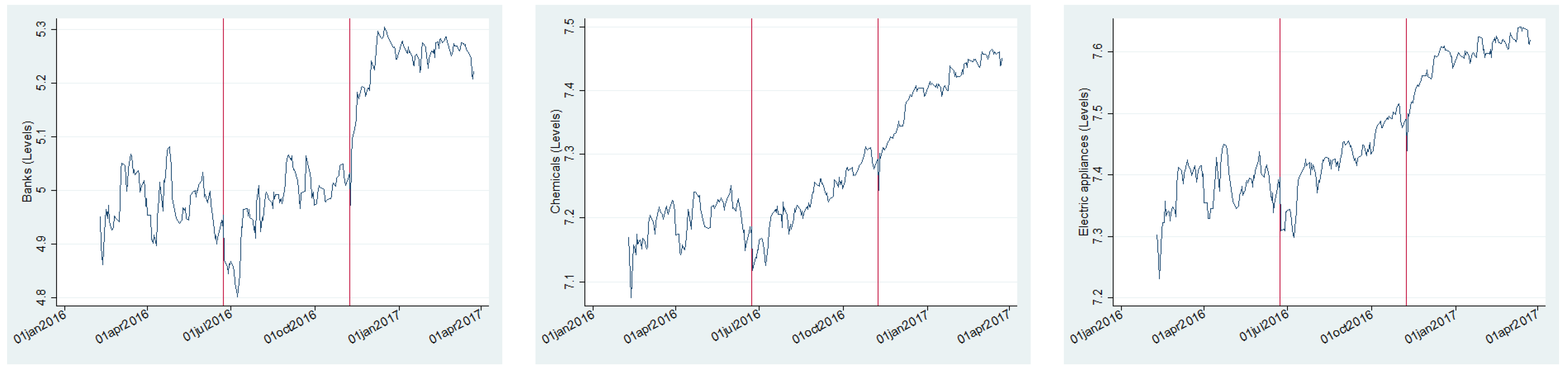
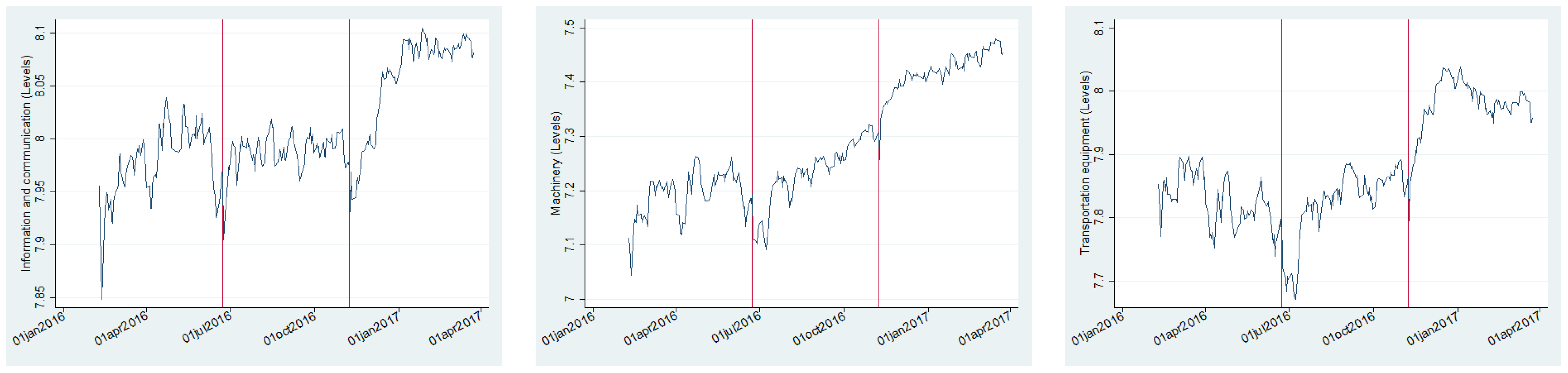
The daily logarithmic returns of the exchange rate of JPY per one USD, the closing price index of Nikkei 225, the closing price index of TOPIX and the closing price of the TOPIX sectoral indices with a weight of 5% and more (banks, chemicals, electric appliances, information and communication, machinery and transportation equipment indices) for the period of 10 February 2016 to 24 March 2017 were used in estimations. The raw data came from the Bank of Japan, TSE and Yahoo Finance.

The explanatory statistics for the logarithmic returns of the variables are presented in

Table 1. Daily logarithmic returns of the exchange rates and stock price indices. Author’s estimations based on the data from the Bank of Japan, TSE and Yahoo Finance. The total number of observations is 275. The maximum number of lags for the augmented Dickey–Fuller (ADF) test selected by the Schwarz–Bayesian information criterion is 15. For the ARCH test, *** indicates that the null hypothesis of no ARCH (1) effects at a 1% significance level is rejected. For the ADF test, *** indicates values less than the critical value at a 1% significance level.

Variables	Mean	Std. Dev.	Skewness	Kurtosis	ARCH	ADF
JPY	−0.0001	0.0084	−0.5475	8.7637	9.646 ***	−3.581 ***
Nikkei	0.0007	0.0148	−0.3276	9.7716	13.284 ***	−5.276 ***
TOPIX	0.0006	0.0142	−0.2021	10.0960	18.392 ***	−5.271 ***
Banks	0.0010	0.0221	0.3557	5.1824	8.840 ***	−4.564 ***
Chemicals	0.0010	0.0147	0.0198	10.0903	31.638 ***	−5.122 ***
Electric appliances	0.0012	0.0162	−0.3415	8.9397	8.608 ***	−5.797 ***
Information and communication	0.0005	0.0138	−0.4502	8.4689	65.590 ***	−4.609 ***
Machinery	0.0012	0.0169	0.1798	8.5559	8.775 ***	−5.100 ***
Transportation equipment	0.0004	0.0188	−0.2496	6.8985	16.651 ***	−4.746 ***

. The mean values are negative for JPY and positive for all other variables. The standard deviation values show higher volatility for stocks, especially for the banks index. The skewness values are positive for the banks, chemicals, and machinery indices and negative for all other variables. All variables have distributions with positive excess kurtosis.

The LM test for ARCH rejects the null hypothesis of no ARCH (1) effects at a 1% significance level for all variables. This means that periods of high and low volatility are grouped together (volatility clustering) and that the ARCH-type models are suitable. The augmented Dickey–Fuller unit root test (Dickey and Fuller 1979, 1981) indicates that all values are less than the critical value at a 1% significance level (Table 1), and the null hypothesis of a unit root is rejected at all common significance levels.

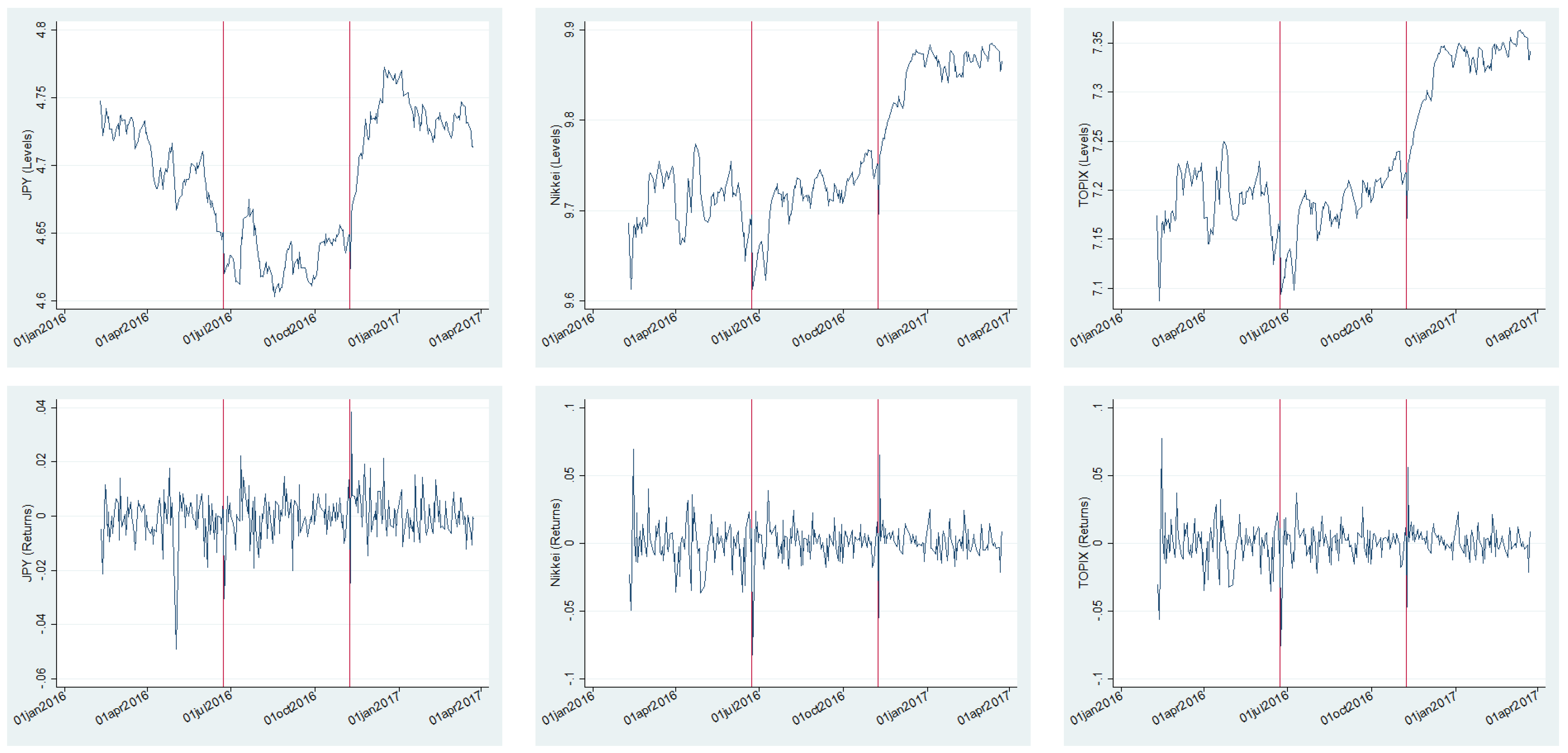
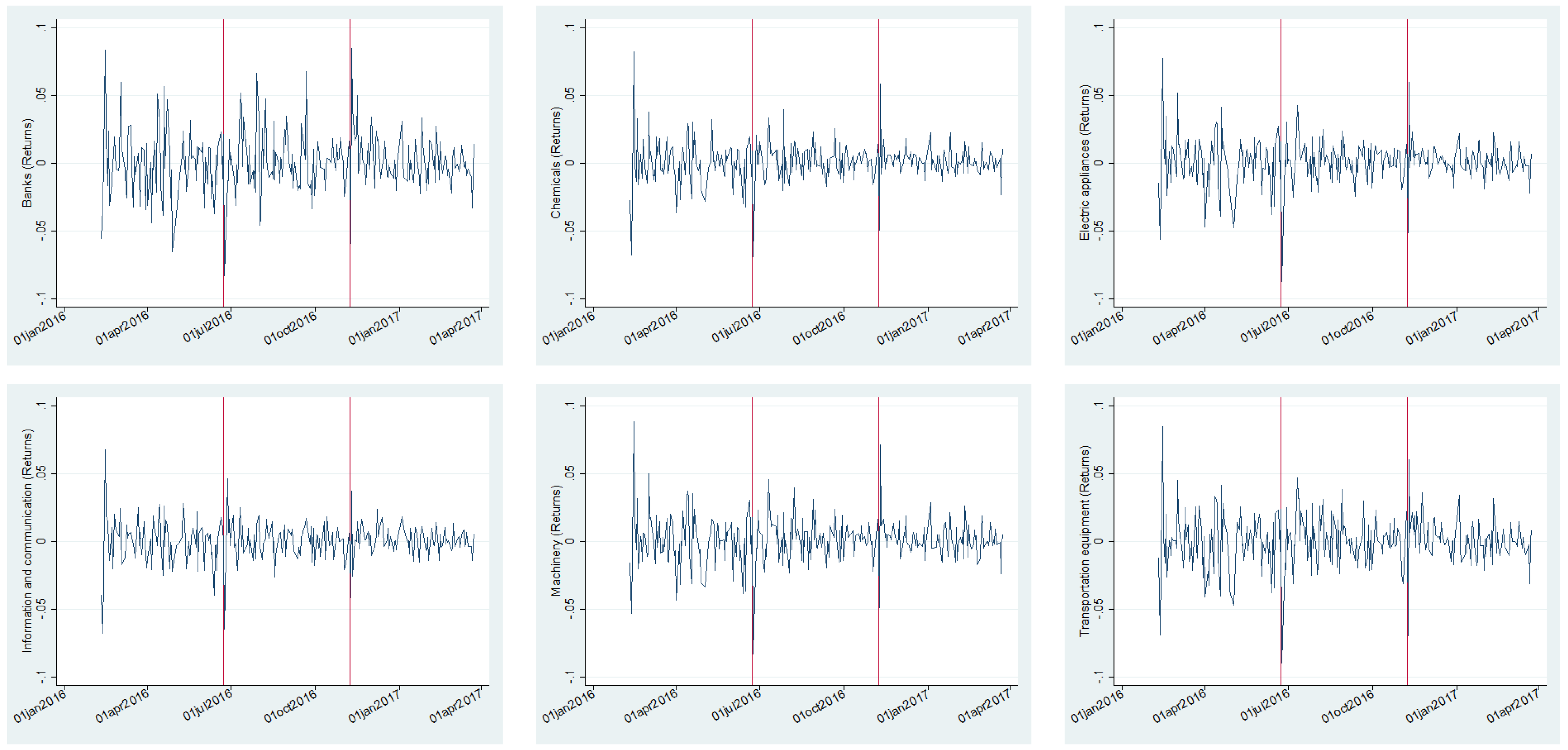
The logarithmic levels and returns of all variables are shown in Figure 1, Figure 2 and Figure 3. The vertical reference lines indicate the day of BR (23 June 2016) and USE (8 November 2016).

The levels demonstrate a structural change in the data after each event, and the returns show higher volatility in the first days following each event. The returns figures clearly indicate stationarity and volatility clustering as reported by the unit root test and the LM test for the ARCH effect.

Additional comments about the changes after each event are provided in the empirical findings. An equal number of observations before and after each event is included in the estimations to make the comparison more robust. This is the reason for the total number of observations of 275.

4. Empirical Findings

4.1. Causality Relationship

The EGARCH estimations for JPY, Nikkei and TOPIX are presented in

Table 2. EGARCH estimation for JPY, Nikkei, and TOPIX. Author’s estimations based on data from the Bank of Japan, TSE, and Yahoo Finance. The numbers in parentheses are standard errors. ***, **, and * indicate significance at the 1%, 5%, and 10% levels, respectively. Distribution is Student’s t. DF means the degree of freedom. Q (5) and Q (10) (and squared Q (5) and Q (10)) are the Ljung–Box Q statistics for the null hypothesis of no autocorrelation of up to orders 5 and 10 for the standardised residuals (and squared standardised residuals).

	JPY	Nikkei	TOPIX
c	−0.0001 (0.0005)	0.0003 (0.0007)	0.0004 (0.0007)
b1	−0.0664 (0.0479)	0.0062 (0.0494)	0.0452 (0.0601)
γ	−0.0274 (0.0341)	−0.3623 *** (0.0887)	−0.2887 *** (0.0893)
α	0.0158 (0.0155)	0.0714 (0.0695)	0.0823 (0.0656)
β1	−1.7211 *** (0.0154)	0.4572 * (0.2437)	0.9519 *** (0.0332)
β2	−0.9915 *** (0.0139)	0.4853 ** (0.2425)
w	−35.1132 *** (0.4625)	−0.5053 * (0.26459)	−0.4319 (0.2927)
Distribution	t	t	t
DF	3.2919 (0.3741)	4.0420 (0.9360)	4.5441 (1.2215)
Q(5)	3.3270 (0.6497)	3.3736 (0.6426)	4.2695 (0.5113)
Q(10)	3.9154 (0.9511)	4.3191 (0.9318)	4.5472 (0.9193)
Q2(5)	0.9971 (0.9628)	0.5432 (0.9905)	2.7771 (0.7343)
Q2(10)	2.9620 (0.9823)	2.5353 (0.9904)	5.1588 (0.8803)

. The asymmetric effect of information on the variance of Nikkei and TOPIX and the effect of the previous periods’ variance on the variance of JPY and stock indices are statistically significant (at 1% to 10% significance levels). The Portmanteau test of white noise for the null hypothesis of no autocorrelation up to order 5 (and 10) for the standardised residuals and their squares proves the absence of autocorrelation.

The EGARCH estimations for the sectoral stock indices are presented in

Table 3. EGARCH estimation for sectoral indices. Author’s estimations based on data from the Bank of Japan, TSE, and Yahoo Finance. The numbers in parentheses are standard errors. ***, **, and * indicate significance at the 1%, 5%, and 10% levels, respectively. Distribution is Student’s t. DF means the degree of freedom. Q (5) and Q (10) (and squared Q (5) and Q (10)) are the Ljung–Box Q statistics for the null hypothesis of no autocorrelation of up to orders 5 and 10 for the standardised residuals (and squared standardised residuals).

	Banks	Chemicals	Electric Appliances	Information and Communication	Machinery	Transportation Equipment
c	−0.0006	0.0008	0.0006	0.0006	0.0007 *	−0.0001
	(0.0006)	(0.0006)	(0.0008)	(0.0007)	(0.0004)	(0.0008)
b1	0.1296 ***	−0.0810 *	0.0068	0.0967	−0.0164	0.0171
	(0.0498)	(0.0472)	(0.0675)	(0.0663)	(0.0466)	(0.0513)
b2					0.0017
					(0.0264)
b3					−0.0736
					(0.0538)
b4					−0.1316 **
					(0.0605)
γ	−0.1450 *	−0.2367 ***	−0.2476 ***	−0.3034 ***	−0.2430 ***	−0.3397 ***
	(0.0819)	(0.0609)	(0.0921)	(0.0923)	(0.0755)	(0.1104)
α	0.2787	−0.0038	0.07249 *	0.1608	0.0444	0.1055
	(0.2872)	(0.0315)	(0.0428)	(0.1305)	(0.0641)	(0.1037)
β1	0.9371 ***	0.9684 ***	0.9780 ***	0.6810 ***	0.9723 ***	0.1491 *
	(0.1795)	(0.0148)	(0.0166)	(0.2334)	(0.0098)	(0.0794)
β2				−0.4795 ***		0.8122 ***
				(0.1587)		(0.0994)
w	−0.4645	−0.2816 **	−0.1915	−6.9824 ***	−0.2338 ***	−0.3206
	(1.3655)	(0.1269)	(0.1363)	(1.3196)	(0.0808)	(0.3287)
Distribution	t	t	t	t	t	t
DF	4.8900	4.7378	5.1727	4.7993	6.3041	5.0432
	(1.2631)	(1.0259)	(1.3770)	(1.4966)	(2.1241)	(1.5570)
Q(5)	5.7046	4.4038	5.2849	4.8950	1.9434	2.6450
	(0.3360)	(0.4929)	(0.3821)	(0.4288)	(0.8569)	(0.7545)
Q(10)	8.9951	7.0046	5.8930	12.6079	4.0141	4.8700
	(0.5326)	(0.7250)	(0.8242)	(0.2464)	(0.9467)	(0.8997)
Q2(5)	2.4709	7.5030	2.7370	0.9249	6.0914	0.1321
	(0.7809)	(0.1858)	(0.7404)	(0.9684)	(0.2974)	(0.9997)
Q2(10)	5.8547	9.0113	5.0946	4.1573	7.2140	1.4642
	(0.8273)	(0.5310)	(0.8848)	(0.9400)	(0.7051)	(0.9990)

. The previous returns have a significant effect on the current returns for the banks (at a 1% significance level), chemicals and machinery indices (at a 5–10% significance level). The asymmetric effect of past information on the variance of all sectoral stock indices, the symmetric effect of past information on the variance of the electric appliances index and the effect of the previous periods’ variance on the variance of all sectoral stock indices are statistically significant at 1–10% significance levels. The Portmanteau test of white noise for the null hypothesis of no autocorrelation up to order 5 for the standardised residuals and their squares proves the absence of autocorrelation.

The highest values of the chi-square test statistics for the hypothesis of no causality in variance from lag 1 to lag 10 among JPY, Nikkei and TOPIX are presented in

Table 4. Causality relationship among JPY, Nikkei, and TOPIX. Author’s estimations. First line reports Hong’s (2001) Q-statistics with truncated kernel. Second line reports Hong’s (2001) Q-statistics with Bartlett kernel. Third line reports cross-correlation coefficients at lag 0 (contemporaneous correlation). *** means that the null hypothesis of no causality (from lag 1 to lag 10 for Hong’s (2001) Q-statistics) at a 1% significance level is rejected.

Causality in Variance
From JPY		From Nikkei		From TOPIX
Nikkei	TOPIX	TOPIX	JPY	Nikkei	JPY
−0.3324	−0.4248	0.3867	21.1677 ***	−0.4863	14.0199 ***
−0.2345	−0.3002	0.2768	15.0518 ***	−0.3439	9.9698 ***
[0.3813 ***]	[0.3883 ***]	[0.9610 ***]	[0.3813 ***]	[0.9610 ***]	[0.3883 ***]

. The test results show causality in variance (volatility spillover) from the stock indices (Nikkei and TOPIX) to JPY. This means that volatility in the stock market overflows to the foreign exchange market within two weeks. As weekends are not included in the estimations, 10 days mean two weeks. Cross-correlation coefficients at lag 0 (contemporaneous correlation) are statistically significant at a 1% significance level.

The highest values of the chi-square test statistics for the hypothesis of no causality in variance from lag 1 to lag 10 from JPY, Nikkei and TOPIX to the sectoral stock indices are presented in

Table 5. Causality from JPY, Nikkei, and TOPIX to sectoral indices. Author’s estimations. First line reports Hong’s (2001) Q-statistics with truncated kernel. Second line reports Hong’s (2001) Q-statistics with Bartlett kernel. Third line reports cross-correlation coefficients at lag 0 (contemporaneous correlation). ***, ** and * indicate that the null hypothesis of no causality (from lag 1 to lag 10 for Hong’s (2001) Q-statistics) at the 1%, 5%, and 10% significance levels, respectively, is rejected.

Causality in Variance
	Banks	Chemicals	Electric appliances	Information and communication	Machinery	Transportation equipment
From JPY	−0.5650	−0.6857	−0.4480	−0.2133	−0.5622	−0.4129
	−0.4318	−0.4857	−0.3167	−0.2898	−0.3979	−0.2917
	[0.3311 ***]	[0.3559 ***]	[0.4531 ***]	[0.3145 ***]	[0.4018 ***]	[0.3884 ***]
From Nikkei	5.5025 ***	1.8915 **	0.9603	−0.6391	1.6758 **	−0.7057
	3.9141 ***	1.3466 *	0.6846	−0.4526	1.1933	−0.4999
	[0.7202 ***]	[0.8184 ***]	[0.9276 ***]	[0.8145 ***]	[0.8485 ***]	[0.9293 ***]
From TOPIX	7.2196 ***	2.1211 **	1.2180	−0.6529	0.6584	−0.6931
	5.1348 ***	1.5099 *	0.8678	−0.4624	0.4700	−0.4909
	[0.7416 ***]	[0.8844 ***]	[0.9379 ***]	[0.8461 ***]	[0.8616 ***]	[0.9086 ***]

. The test results show causality in variance from Nikkei and TOPIX to the banks and chemicals indices and from Nikkei to the machinery index. Cross-correlation coefficients at lag 0 (contemporaneous correlation) are statistically significant at a 1% significance level.

The highest values of the chi-square test statistics for the hypothesis of no causality in variance from lag 1 to lag 10 from the sectoral indices to JPY, Nikkei and TOPIX are presented in

Table 6. Causality from sectoral indices to JPY, Nikkei, and TOPIX. Author’s estimations. First line reports Hong’s (2001) Q-statistics with truncated kernel. Second line reports Hong’s (2001) Q-statistics with Bartlett kernel. Third line reports cross-correlation coefficients at lag 0 (contemporaneous correlation). ***, ** and * indicate that the null hypothesis of no causality (from lag 1 to lag 10 for Hong’s (2001) Q-statistics) at the 1%, 5%, and 10% significance levels, respectively, is rejected.

Causality in Variance
Banks	Chemicals	Electric appliances	Information and communication	Machinery	Transportation equipment
17.5604 ***	10.2060 ***	7.2746 ***	3.4492 ***	24.4382 ***	10.7847 ***	to JPY
12.4870 ***	7.2581 ***	5.1740 ***	2.4542 ***	17.3771 ***	7.6696 ***
[0.3311 ***]	[0.3559 ***]	[0.4531 ***]	[0.3145 ***]	[0.4018 ***]	[0.3884 ***]
−0.6622	−0.2402	−0.4703	−0.2903	−0.6634	−0.3834	to Nikkei
−0.4690	−0.1690	−0.3325	−0.2045	−0.4698	−0.2708
[0.7202 ***]	[0.8184 ***]	[0.9276 ***]	[0.8145 ***]	[0.8485 ***]	[0.9293 ***]
−0.7030	1.9366 **	0.6036	1.7935 **	−0.2702	0.5561	to TOPIX
−0.4980	1.3787 *	0.4310	1.2770	−0.1903	0.3972
[0.7416 ***]	[0.8844 ***]	[0.9379 ***]	[0.8461 ***]	[0.8616 ***]	[0.9086 ***]

. The test results show causality in variance from all sectoral indices to JPY and from the chemicals and information and communication indices to TOPIX. Cross-correlation coefficients at lag 0 (contemporaneous correlation) are statistically significant at a 1% significance level.

The highest values of the chi-square test statistics for the hypothesis of no causality in variance from lag 1 to lag 10 among the sectoral indices are presented in

Table 7. Causality relationship among sectoral indices. Author’s estimations. First line reports Hong’s (2001) Q-statistics with truncated kernel. Second line reports Hong’s (2001) Q-statistics with Bartlett kernel. Third line reports cross-correlation coefficients at lag 0 (contemporaneous correlation). ***, ** and * indicate that the null hypothesis of no causality (from lag 1 to lag 10 for Hong’s (2001) Q-statistics) at the 1%, 5%, and 10% significance levels, respectively, is rejected.

Causality in Variance
	Banks	Chemicals	Electric appliances	Information and communication	Machinery	Transportation equipment
From banks		−0.5309	−0.4850	−0.4565	0.5813	−0.6673
		−0.3757	−0.3430	−0.3227	0.4152	−0.4726
		[0.5692 ***]	[0.6955 ***]	[0.5061 ***]	[0.7297 ***]	[0.6845 ***]
From chemicals	13.3011 ***		2.3703 ***	−0.6695	0.8505	−0.6873
	9.4587 ***		1.6870 **	−0.4742	0.6065	−0.4868
	[0.5692 ***]		[0.8623 ***]	[0.7796 ***]	[0.8936 ***]	[0.7740 ***]
From electric appliances	6.9009 ***	1.4654 *		−0.6391	0.9280	−0.7067
	4.9083 ***	1.0437		−0.4526	0.6617	−0.5006
	[0.6955 ***]	[0.8623 ***]		[0.7614 ***]	[0.8782 ***]	[0.8805 ***]
From information and communication	9.5706 ***	2.9746 ***	1.8289 **		−0.0698	−0.6657
	6.8064 ***	2.1168 **	1.3021 *		−0.0724	−0.4714
	[0.5061 ***]	[0.7796 ***]	[0.7614 ***]		[0.6259 ***]	[0.8039 ***]
From machinery	4.0130 ***	1.4286 *	0.3548	−0.7006		−0.8512
	2.8550 ***	1.0175	0.2541	−0.4963		−0.4581
	[0.7297 ***]	[0.8936 ***]	[0.8782 ***]	[0.6259 ***]		[0.7845 ***]
From transportation equipment	4.5357 ***	1.8378 **	0.6781	−0.5105	0.8926
	3.2266 ***	1.3085 *	0.4839	−0.3611	0.6364
	[0.6845 ***]	[0.7740 ***]	[0.8805 ***]	[0.8039 ***]	[0.7845 ***]

. The test results show causality in variance from all sectoral indices to the banks index. Causality in variance is also detected from the sectoral indices (excluding banks index) to the chemicals index and from the chemicals and information and communication indices to the electric appliances index. Cross-correlation coefficients at lag 0 (contemporaneous correlation) are statistically significant at a 1% significance level.

The unidirectional causality in variance among the variables derived from the estimations is shown in Figure 4.

Considering the direction of causality, volatility may spread indirectly among the variables as follows: from Nikkei to JPY through the banks index; from Nikkei to the banks index, electric appliances index, JPY and TOPIX through the chemicals index; from Nikkei to the banks index, chemicals index and JPY through the machinery index; from TOPIX to JPY through the banks index; from TOPIX to the banks index, electric appliances index and JPY through the chemicals index; from the chemicals index to JPY through the banks index; from the chemicals index to the banks index and JPY through the electric appliances index; from the chemicals index to the banks index and JPY through TOPIX; from the electric appliances index to JPY through the banks index; from the electric appliances index to the banks index, JPY and TOPIX through the chemicals index; from the information and communication index to JPY through the banks index; from the information and communication index to the banks index, electric appliances index, JPY and TOPIX through the chemicals index; from the information and communication index to the banks index, chemicals index and JPY through the electric appliances index; from the information and communication index to the banks index, chemicals index and JPY through TOPIX; from the machinery index to JPY through the banks index; from the machinery index to the banks index, electric appliances index, JPY and TOPIX through the chemicals index; from the transportation equipment index to JPY through the banks index; from the transportation equipment index to the banks index, electric appliances index, JPY and TOPIX through the chemicals index.

4.2. Effect of BR and USE

Important international events exposing new information to the market change investors’ beliefs and affect the volatility of financial indicators. The effect is more substantial if the results are unanticipated. Figure 1 and Figure 2 in Section 3 illustrate the changes in levels for all variables after BR and USE, two important international events with unpredictable results. The levels have an increasing trend for the period after BR and USE (excluding JPY after BR), following a sharp fall in the first days after each event. The logarithmic returns (Figure 1 and Figure 3) show obvious instability for all variables in the first days after each event.

The comparison of the mean and standard deviation of the logarithmic returns for five days before and after BR and USE (

Table 8. Mean and standard deviation for five days before and after each event. Author’s estimations based on the data from the Bank of Japan, TSE and Yahoo Finance.

Variables	Before BR		After BR		Before USE		After USE
	Mean	Std. Dev.	Mean	Std. Dev.	Mean	Std. Dev.	Mean	Std. Dev.
JPY	−0.0001	0.0033	−0.0034	0.0156	−0.0007	0.0090	0.0065	0.0224
Nikkei	0.0102	0.0106	−0.0083	0.0426	−0.0029	0.0133	0.0057	0.0430
TOPIX	0.0090	0.0107	−0.0083	0.0387	−0.0043	0.0124	0.0057	0.0369
Banks	0.0109	0.0138	−0.0186	0.0382	−0.0034	0.0163	0.0204	0.0520
Chemicals	0.0075	0.0105	−0.0072	0.0356	−0.0037	0.0116	0.0028	0.0394
Electric appliances	0.0115	0.0142	−0.0114	0.0444	−0.0051	0.0129	0.0054	0.0406
Information and communication	0.0086	0.0074	0.0003	0.0407	−0.0070	0.0113	−0.0057	0.0300
Machinery	0.0120	0.0150	−0.0122	0.0411	−0.0029	0.0139	0.0107	0.0427
Transportation equipment	0.0141	0.0133	−0.0215	0.0419	−0.0054	0.0224	0.0046	0.0470

) shows a decrease in the mean and an increase in volatility after BR and an increase in the mean and volatility after USE for all variables.

To precisely measure the effect of BR and USE on the variables used in estimations, we incorporate dummy variables into the mean and variance equations (Equations (1) and (2)) for the first five days after each event. As weekends are not included, five days mean a week in this paper. The estimation results are presented in

Table 9. EGARCH estimation with dummy variables for BR and USE. Author’s estimations based on the data from the Bank of Japan, TSE and Yahoo Finance. The numbers in parentheses are standard errors. ***, ** and * indicate significance at the 1%, 5% and 10% levels, respectively. Distribution is Student’s t. DF means the degree of freedom.

	JPY	Nikkei	TOPIX	Chemicals	Electric Appliances	Transportation Equipment
c	−0.0002	0.0009	0.0005	0.0001	0.0007	0.0003
	(0.0005)	(0.0007)	(0.0007)	(0.0007)	(0.0008)	(0.0009)
b1	−0.1035 *	0.0145	0.0540	−0.0624	0.0269	0.0216
	(0.0619)	(0.0471)	(0.0639)	(0.0705)	(0.0840)	(0.0549)
BR	0.0002	0.0032	−0.0028	0.0005	−0.0039	−0.0112
	(0.0023)	(0.0054)	(0.0161)	(0.0117)	(0.0178)	(0.0131)
USE	0.0108 ***	0.0058	0.0013	−0.0052	−0.0022	0.0100
	(0.0037)	(0.0082)	(0.0103)	(0.0187)	(0.0134)	(0.0076)
γ	0.0539	−0.1972	−0.2988 **	−0.3085 ***	−0.2557 ***	−0.2041 **
	(0.0741)	(0.1227)	(0.1337)	(0.0785)	(0.0989)	(0.0932)
α	−0.0145	0.0218	0.1256	−0.0789	0.0691	0.1934
	(0.0705)	(0.1656)	(0.1737)	(0.0546)	(0.0597)	(0.1317)
β1	−0.2196 **	−0.0580	0.9494 ***	0.9797 ***	0.9863 ***	−0.1053
	(0.1022)	(0.1080)	(0.0702)	(0.0115)	(0.0197)	(0.1704)
β2	−0.8501 ***	−0.7298 ***				−0.6788 ***
	(0.0904)	(0.1007)				(0.1706)
BR	1.8513	2.9336 ***	−0.1928	−0.2335	−0.1760	3.3768 ***
	(1.3388)	(1.0416)	(0.4378)	(0.1778)	(0.2610)	(0.8696)
USE	2.3353 ***	2.8674 ***	−0.1462	0.2144	−0.0668	2.3588 ***
	(0.7809)	(0.7408)	(0.4999)	(0.4200)	(0.3039)	(0.8206)
w	−20.0846 ***	−15.3503 ***	−0.4479	−0.1728 *	−0.1161	−14.5654 ***
	(1.7831)	(1.5100)	(0.6196)	(0.1014)	(0.1688)	(2.2080)
Distribution	t	t	t	t	t	t
DF	4.2837	3.4714	4.6088	6.2277	5.5150	5.7447
	(1.1952)	(1.0873)	(1.1646)	(2.3764)	(1.4576)	(2.7527)

.

Owing to the flat log pseudolikelihood, the software (Stata 14.2) cannot estimate the mean and variance equations with dummy variables for the banks, information and communication and machinery indices. The estimations for the other variables show a significant positive effect of BR at a 1% significance level on the variances of Nikkei and the transportation equipment index. A significant positive effect at a 1% significance level is found from USE to the returns of JPY and the variances of JPY, Nikkei and the transportation equipment index. Accordingly, BR and USE cause instability (i.e., an increase in volatility) to Nikkei and the transportation equipment index in the first week. USE also causes instability (i.e., an increase in volatility) to JPY.

Considering the presence of volatility overflow among the variables, as shown in Figure 4, we suggest that BR and USE also affect other variables indirectly through volatility spillover. BR and USE may indirectly affect the volatility of JPY, the banks and chemicals indices through Nikkei and the transportation equipment index. BR and USE may also indirectly affect the volatility of the machinery index through Nikkei.

5. Conclusions

Financial variables, particularly foreign exchange and stock price indices, are very sensitive to domestic and international economic and political changes. Developments in information and telecommunication technologies have accelerated the flow of information and its effect on the expectations of investors and, consequently, on financial markets. Volatility overflow among financial variables, which adds an indirect effect of external factors to their direct effect, increases instability in financial markets and makes portfolio management and decision making difficult for investors and policymakers.

In this study, we examined the changes in volatility overflow among JPY, Nikkei, TOPIX and the TOPIX sectoral indices. The findings highlighted causality in variance (volatility spillover) among the variables. We revealed that volatility could also spread indirectly among the variables (from one variable to another through a third variable).

During the estimated period, two important international economic and political events, BR and USE, took place. The comparison of the mean and standard deviation of the logarithmic returns for five days before and after BR and USE showed changes in the mean and an increase in instability after both events. The estimations demonstrated a significant direct effect from the external shocks on the exchange rates of JPY, Nikkei and the transportation equipment index. Considering the presence of causality in variance from Nikkei and the transportation equipment index to the other variables, we suggest that external shocks may also affect other variables indirectly through volatility overflow.

The paper is distinct from previous studies in two main ways. First, it incorporates the causality relationship for sectoral stock indices, making the results more informative. Second, it considers the indirect impact of internal and external shocks through volatility transmission.

The findings regarding the effect of external shocks on the returns, volatility, and volatility spillover among the sectoral stock indices and between the sectoral indices and major financial indicators further contribute to the literature on Japanese financial markets. Future studies related to this paper can explore other volatility spillover methodologies and can extend the research to other sectoral indices and internal and external shocks, particularly the impact of the Coronavirus disease 2019 (COVID-19) pandemic.

References

1. Agren, Martin. 2006. Does Oil Price Uncertainty Transmit to STOCK Markets? Working Paper Series 2006: 23; Uppsala: Uppsala University, Department of Economics. [Google Scholar]
2. Bank for International Settlements. 2019. Triennial Central Bank Survey-Foreign Exchange Turnover in April 2019. Available online: https://www.bis.org/statistics/rpfx19_fx.pdf (accessed on 2 September 2021).
3. Bashir, Usman, Gilney Figueira Zebende, Yugang Yu, Muntazir Hussain, Ahmed Ali, and Ghulam Abbas. 2019. Differential market reactions to pre and post Brexit referendum. Physica A: Statistical Mechanics and its Applications 515: 151–58. [Google Scholar] [CrossRef]
4. Belke, Ansgar, Irina Dubova, and Thomas Osowski. 2018. Policy uncertainty and international financial markets: The case of Brexit. Applied Economics 50: 3752–70. [Google Scholar] [CrossRef] [Green Version]
5. Bollerslev, Tim. 1986. Generalised autoregressive conditional hetroscedasticity. Journal of Econometrics 31: 307–27. [Google Scholar] [CrossRef] [Green Version]
6. Box, George, and David Pierce. 1970. Distribution of residual autocorrelations in autoregressive-integrated moving average time series models. Journal of the American Statistical Association 65: 1509–26. [Google Scholar] [CrossRef]
7. Cheung, Yin-Wong, and Lilian K. Ng. 1996. A causality-in-variance test and its application to financial market prices. Journal of Econometrics 72: 33–48. [Google Scholar] [CrossRef]
8. Chung, Chae-Shik, and Youngmin Jang. 2000. Analysis of changes in the relationship between the KRW/USD exchange rate and JPY/USD exchange rate before and after the economic crisis. East Asian Economic Review 4: 65–93. [Google Scholar] [CrossRef]
9. Dickey, Alan Dickey, and Wayne Arthur Fuller. 1979. Distribution of the estimators for autoregressive time series with a unit root. Journal of the American Statistical Association 74: 427–31. [Google Scholar]
10. Dickey, Alan Dickey, and Wayne Arthur Fuller. 1981. Likelihood ration statistics for autoregressive time series with a unit root. Econometrica 49: 1057–72. [Google Scholar] [CrossRef]
11. Diebold, Francis, and Kamil Yilmaz. 2012. Better to give than to receive: Predictive directional measurement of volatility spillovers. International Journal of Forecasting 28: 57–66. [Google Scholar] [CrossRef] [Green Version]
12. Engle, Fry Robert. 1982. Autoregressive conditional heteroskedasticity with estimates of the variance of United Kingdom inf1ation. Econometrica 50: 987–1007. [Google Scholar] [CrossRef]
13. Hamori, Shigeyuki. 2003. An Empirical Investigation of Stock Markets: The CCF Approach. New York: Springer Science, Business Media. [Google Scholar]
14. Hanabusa, Kunihiro. 2010. Effects of foreign disasters on the petroleum industry in Japan: A financial market perspective. Energy 35: 5455–63. [Google Scholar] [CrossRef]
15. Hong, Yongmiao. 2001. A test for volatility spillover with application to exchange rates. Journal of Econometrics 103: 183–224. [Google Scholar] [CrossRef]
16. Joseph, Treesa, and Anjali Verma. 2018. Driver-driven relationship between the Tokyo Stock Exchange indices-TOPIX and Nikkei. Asian Journal of Management 9: 1319–24. [Google Scholar] [CrossRef]
17. Kadiric, Samir, and Arthur Korus. 2019. The effects of Brexit on credit spreads: Evidence from UK and Eurozone corporate bond markets. International Economics and Economic Policy 16: 65–102. [Google Scholar] [CrossRef] [Green Version]
18. Karfakis, Costas, and Theodore Panagiotidis. 2015. The effects of global monetary policy and Greek debt crisis on the dynamic conditional correlations of currency markets. Empirica (Journal of European Economics) 42: 795–811. [Google Scholar] [CrossRef]
19. Lin, Chin-Tsai, and Yi-Hsien Wang. 2005. An analysis of political changes on Nikkei 225 stock returns and volatilities. Annals of Economics and Finance 6: 169–83. [Google Scholar]
20. Ljung, Greta, and George Box. 1978. On a measure of lack of fit in time series models. Biometrika 65: 297–303. [Google Scholar] [CrossRef]
21. Mandelbrot, Benoit. 1996. The variation of certain speculative prices. The Journal of Business 36: 394–419. [Google Scholar] [CrossRef]
22. Nelson, Daniel. 1991. Conditional heteroskedasticity in asset returns: A new approach. Econometrica 59: 347–70. [Google Scholar] [CrossRef]
23. Sato, Setsuya. 2021. New Perspectives on Globalization: Developing Global Literacy to Catch Up with the Global Trend. Tokyo: Bungeisha. [Google Scholar]
24. Shaikh, Imlak. 2017. The 2016 U.S. presidential election and the stock, FX and VIX markets. The North American Journal of Economics and Finance 42: 546–63. [Google Scholar] [CrossRef]
25. Sultonov, Mirzosaid, and Nayyar S. Jehan. 2018. Dynamic linkages between Japan’s foreign exchange and stock markets: Response to the Brexit referendum and the 2016 US presidential election. Journal of Risk and Financial Management 11: 34. [Google Scholar] [CrossRef] [Green Version]
26. Sultonov, Mirzosaid. 2020. The impacts of international political and economic events on Japanese financial markets. International Journal of Financial Studies 8: 43. [Google Scholar] [CrossRef]
Figure 1. Levels and returns of JPY, Nikkei and TOPIX. Author’s estimations based on the data from the Bank of Japan, TSE and Yahoo Finance. The levels are the logarithmic values of the variables. The returns are the daily logarithmic differences of the variables.
Jrfm 14 00560 g001
Figure 2. Levels of sectoral indices. Author’s estimations based on the data from the TSE. The levels are the logarithmic values of the variables.
Jrfm 14 00560 g002aJrfm 14 00560 g002b
Figure 3. Returns of sectoral indices. Author’s estimations based on the data from the TSE. The returns are the daily logarithmic differences of the variables.
Jrfm 14 00560 g003
Figure 4. Author’s estimations based on the data from the Bank of Japan, TSE and Yahoo Finance. The arrows show the direction of causality in variance.
Jrfm 14 00560 g004