Article

Technical Analysis of Tourism Price Process in the Eurozone

1
Faculty of Business and Management Sciences, University of Novo Mesto, Na Loko 2, SI-8000 Novo Mesto, Slovenia
2
Faculty of Management, University of Primorska, Izolska vrata 2, SI-6101 Koper, Slovenia
*
Author to whom correspondence should be addressed.
J. Risk Financial Manag. 2021, 14(11), 517; https://doi.org/10.3390/jrfm14110517
Submission received: 2 September 2021 / Revised: 30 September 2021 / Accepted: 19 October 2021 / Published: 27 October 2021
(This article belongs to the Special Issue Technical Analysis of Financial Markets)

Abstract

:
This study is a specific contribution to investigating normalities in prices to a well-established cointegrated vector autoregressive model (VAR). While the role of prices in computational economics has been investigated, the real prices vis-à-vis nominal prices in the decision process has been neglected. The paper investigates the transition from nominal to real time-series of prices without losing information in the data set when deflating or de-seasonalizing. The likelihood approach is based on careful specifications of the (co)integration characteristics of tourism prices. The results confirm that the transmission of tourism prices in the Eurozone positively impacts Slovenian tourism prices when the spatial consolidated cointegrated VAR model is used. The theoretical-conceptual and empirical contribution is twofold: first, the study develops and empirically applies bona fide divisor of normality consolidation for time-series in levels instead of routinely utilised inflation integers, and second, the study introduces perfection of prices on a long-run time-series treatment.

1. Introduction

This paper is inspired by Johansen (2019) and Juselius (2009, 2021) study on the cointegration method and its application in economic applied research. We start with a theoretical explanation of the normalities and applied examples of one country, robustly extended to five countries of the Eurozone. The research aims to maintain normality in time-series, which is usually a complex question. Therefore, scholars using applied methods usually omit the question of normality in time-series after testing for autocorrelation and homoscedasticity. Nevertheless, the normality problem is usually solved incorrectly by increasing the lag length, as Kongsted (2005) discussed. In this paper, we theoretically investigate how to maintain the normalities in the volatilities of tourism prices using the restricted vector autoregressive (VAR) model, with robust tests in a case of a small open economy where tourism plays a significant role in the economy.
The identified research gap has been discussed in the literature, but more often theoretically and less with an applied case study. Therefore, we aim to close the gap in the literature by showing the importance of normalities in tourism price time-series. While volatility is high in financial time-series, prices are treated as I ( 2 ) and inflation as I ( 1 ) (see Appendix B).
The guiding theory used for this study comes from the paper by Archontakis and Mosconi (2021) that is based on the tradition of Katarina Juselius and Søren Johansen.
The paper is novel in two respects. First, it introduces the idea of achieving normality in the time-series, which has been largely neglected in economic research, especially in tourism. Second, it tests the current development of the time-series methodology for robustness and validity using a small open economy data sample, i.e., Slovenia, on a data vector from 2000 to 2012. This period captures volatilities caused by the integration of Slovenia in the EU in 2004, the introduction of the Euro in Slovenia in 2007, and the financial and economic crisis with the recessions in 2009 and 2012.
A unique contribution is to extend the theory and applied economics on the importance of normalities by using multiple misspecification tests instead of simple diagnostic tests to obtain the normally distributed model. Representing nominal and real calculated divisors is a unique approach. The most commonly used visual CVAR representation can be found in Appendix C. Three hypotheses are tested for Slovenian tourism prices, Eurozone tourism prices, and inflation.
The empirical results are based on the cointegration technique of technical analysis of prices. The main focus is on normally distributed residuals and valid predictions based on past data modelling of statistical and econometric trends in tourism prices.
The rest of the paper is divided into four parts: hypotheses development, the methods and data used, the results section, and the discussion, limitations, and conclusions section.

2. Hypothesis and Conceptual Model Development

This paper aims to develop a contemporary approach to seasonal determined tourism prices in computational economics (Jawadi 2020). Seasonal nonstationary time-series were already discussed by Cubadda (1999) and Ma et al. (2016), using panels by Ridderstaat and Croes (2020) and sustainable evolution of seasonality by Martín Martín et al. (2020). The multivariate vector autoregressive (VAR) model (Polito and Wickens 2012) builds on Gaussian—normally distributed (i.i.d.) errors that have often been used as a popular method for an explanation of macroeconomic time-series data started in tourism and hospitality by Wong and Song (2006). Another model often used to analyse and predict price volatility is the generalised-autoregressive-conditional-heteroskedasticity (GARCH) method (Chen et al. 2020; Naimoli and Storti 2021; Bago et al. 2021). The variance in errors is often relatively high in both models. Kristjanpollera and Minutolo (2015) apply an Artificial Neural Network (ANN) to the GARCH method generating an ANN–GARCH. In addition, research is being conducted to improve models that use various techniques, such as the autoregressive moving average (ARIMA) model popularised by Chen et al. (2008) and Bauer et al. (2020), which was developed to predict prices in the tourism-transportation sector (Syriopoulos et al. 2021), and the seasonal ARIMA developed by Ma et al. (2016). This article extends the applied econometrics in the field of unit root discussed by Cubadda (1999) and Polito and Wickens (2012). They were studying the VAR disturbances’ correlation structure and the VAR’s transformation (Clark and Ravazzolo 2015; Franchi and Paruolo 2021; Hoover and Juselius 2015, p. 253). The recent approach concerns seasonal determined tourism prices by transforming integrated nominal seasonal prices to real ones according to their shocks and the waves in macroeconomic determinants (Dritsakis 2004; Kim et al. 2019).
Song et al. (2009) described econometric empirical approaches in the tourism technical analysis. The results show that the forecasts produced using current methods in the scope of cointegration, vector error correction models (VECM), and methodological developments are more precise than those generated by least squares regression models (Victor et al. 2021). Johansen (2012, p. 48); Johansen and Nielsen (2018); Bianchi and Chen (2020); Juselius (2015, p. 213) and Cheng et al. (2021) debated spurious regression and correlation and have applied these two approaches in order to contrast them. This gap is an area of research where cointegration analysis comes in as a chance to model the nonstationarity variation of the data and non-normality of the model (Cubadda 1999). Nonetheless, Schild and Schweikert (2019) define the direction of the pricing approach using cointegration and a way to make conservative decisions when dealing with probabilities.
Narayan (2003) introduces the VAR model in tourism demand modelling. Our article examines the long-run relationship between the real prices, which contributes to the formation of the nominal seasonally determined tourism or hospitality industry prices in a VAR model (Juselius 2009, p. 21). Gričar and Bojnec (2018) discuss cointegration analysis and the long-run relation among several economic and tourism variables. Ridderstaat and Croes (2020) have already addressed an obvious path in seasonal patterns, primarily in disciplines like tourism. However, more robust patterns are needed for testing. Moreover, Johansen and Nielsen (2018) present a fractional CVAR model; on the other hand, this (research introduces a spatial consolidated CVAR model.
The main novelty and contribution are in the empirical testing of the hypotheses set with the applied cointegration approach (Archontakis and Mosconi 2021) to seasonally determined tourism prices by the imperative transformation of integrated nominal to real data vector in the VAR approach. The empirical part of this article introduces the analysis of the transmission of the eurozone price indices in the hospitality industry on Slovenian ones as its member state. The relation of the tourism prices in Slovenia follows the theory of the true and observational variable, unit root econometrics (Hoover and Juselius 2015) in white noise, autoregressions up to second-order integration (Chang 2000), and time-series analysis (Johansen and Nielsen 2018).
So far, no similar study is relevant for theoretical and empirical research on an applied approach to real tourism prices with a unit root econometric theory in tourism. Moreover, we further discuss Hoover and Juselius’s (2015) theoretical model versus empirical reality. Research by Martins et al. (2017), for the first time in empirical tourism (macro)economics, discusses the importance of real prices included in the analyses.
In a free-market economy in the tradable and non-tradable sectors, the prices (Kristjanpollera and Minutolo 2015) reflect an interaction between supply and demand aggregates. In addition, the price may be influenced by other determinants, including policy and other government regulations. The price index is a weighted mean (average) of the products and services in the selected industrial sector in the selected period. The price indices can be statistically analysed among periods or across markets in spatial geographical locations. A consumer price index or consumer prices calculate differences in the price level of products and services in final household consumption in time t . Lower-level indices such as hospitality industry prices and food and beverage ones are defined from a base of these products and services as a part of the consumer price index.
The technical analysis of tourism prices has brought significant innovations. Our article develops a theoretical-conceptual model of nominal vs. real price transformation and its empirical testing. The focus of the analysis is on the Eurozone prices, including the Slovenian hospitality industry prices. Time-series variables are suitable for prediction only in a well-defined stochastic model (Clark and Ravazzolo 2015). Shocks in a model of the observed time-series can be used to test a theoretical-conceptual model (Camarero et al. 2020). This approach can work well as long as critical features of the theory are preserved to confirm both the theoretical model and the model of the true variables (Hoover and Juselius 2015; Archontakis and Mosconi 2021).
This study further develops approaches started by Gričar and Bojnec (2012) or Pacifico (2021). It uses a VAR model with some degree of integration discussed by Franchi and Paruolo (2021) with real variables of practical importance (Błażejowski et al. 2020; Gricar et al. 2021). While normality has mainly been neglected in time-series (Juselius 2021), this research tests for (non)normalities and applies them theoretically (Braione and Scholtes 2016; Cheng et al. 2021; Desgagné and de Micheaux 2018). Moreover, a robust test is conducted to present this theoretical comparison with VAR modelling using a small open country case study (Gjelsvik et al. 2020). The first hypothesis (H1) investigates the eurozone price transmission to the Slovenian price indices in the hospitality industry:
Hypothesis 1 (H1).
The Slovenian price indices in the hospitality industry directly and positively converge to the consumer price indices in the Eurozone and the eurozone price indices in the hospitality industry.
The second hypothesis (H2) tests the input cost-push on the Slovenian price indices in the hospitality industry. In the medium to long run, prices of agro-food commodities traded on domestic and international markets, which appears for input costs in the hospitality industry, might increase at a rate exceeding that of inflation (Bakucs et al. 2012). The input cost-push on the hospitality industry prices is tested by the following hypothesis (H2):
Hypothesis 2 (H2).
The Slovenian price indices in the hospitality industry are linearly positively associated with the Slovenian food and beverages price indices, representing input costs in the hospitality industry.
The third hypothesis (H3) investigates catching up and the convergence of the Slovenian prices to a higher level of the Eurozone prices. The gap in relative price levels between richer, older EU countries and poorer, new EU countries might cause consumer price index adjustment in a direction whereby poorer countries tend to have higher inflation rates than do more prosperous countries. If new accession countries join the European Monetary Union (EMU) and experience a period of accelerated growth as they catch up to more prosperous EU countries, they should expect inflation pressure. Juselius (2009) argues that there is a difference in productivity and prices among old and new EU member states with expected faster price growth in the latter. Therefore, the following hypothesis is developed on the association between the Slovenian and the average Eurozone inflation:
Hypothesis 3 (H3).
Slovenian consumer price indices and consumer price indices in the Eurozone are converging in the long run.

3. Materials and Methods

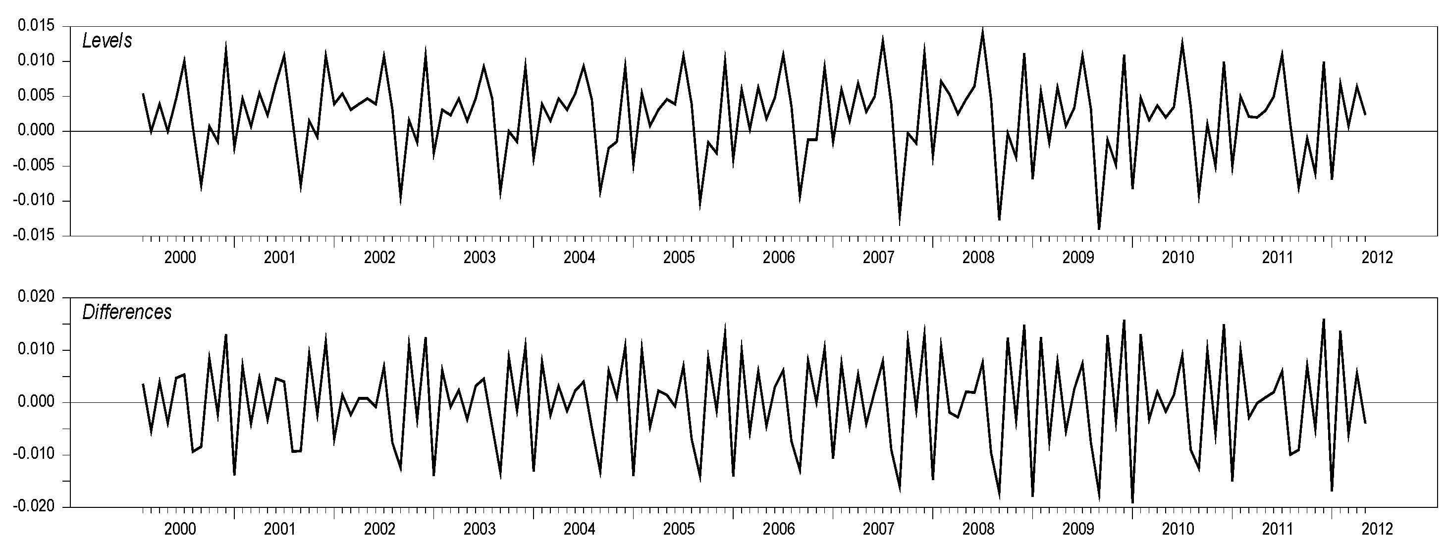
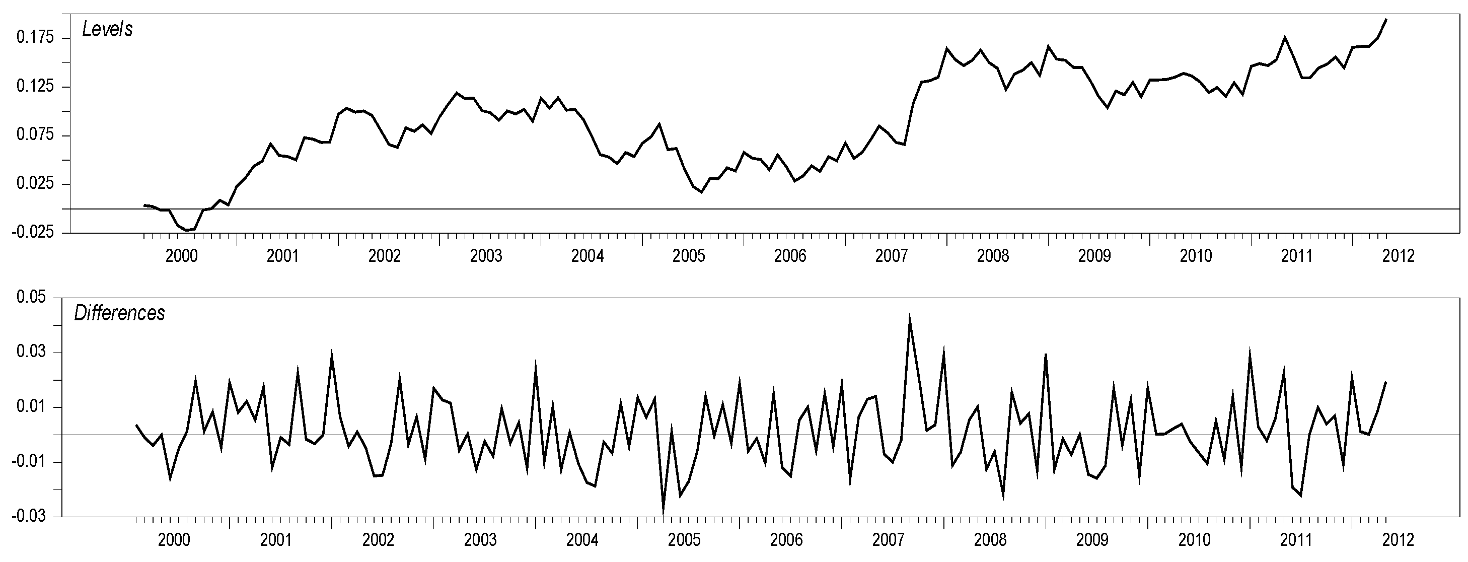
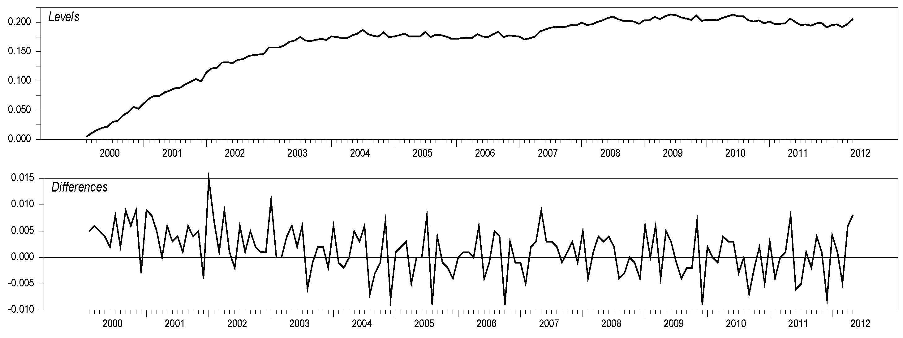
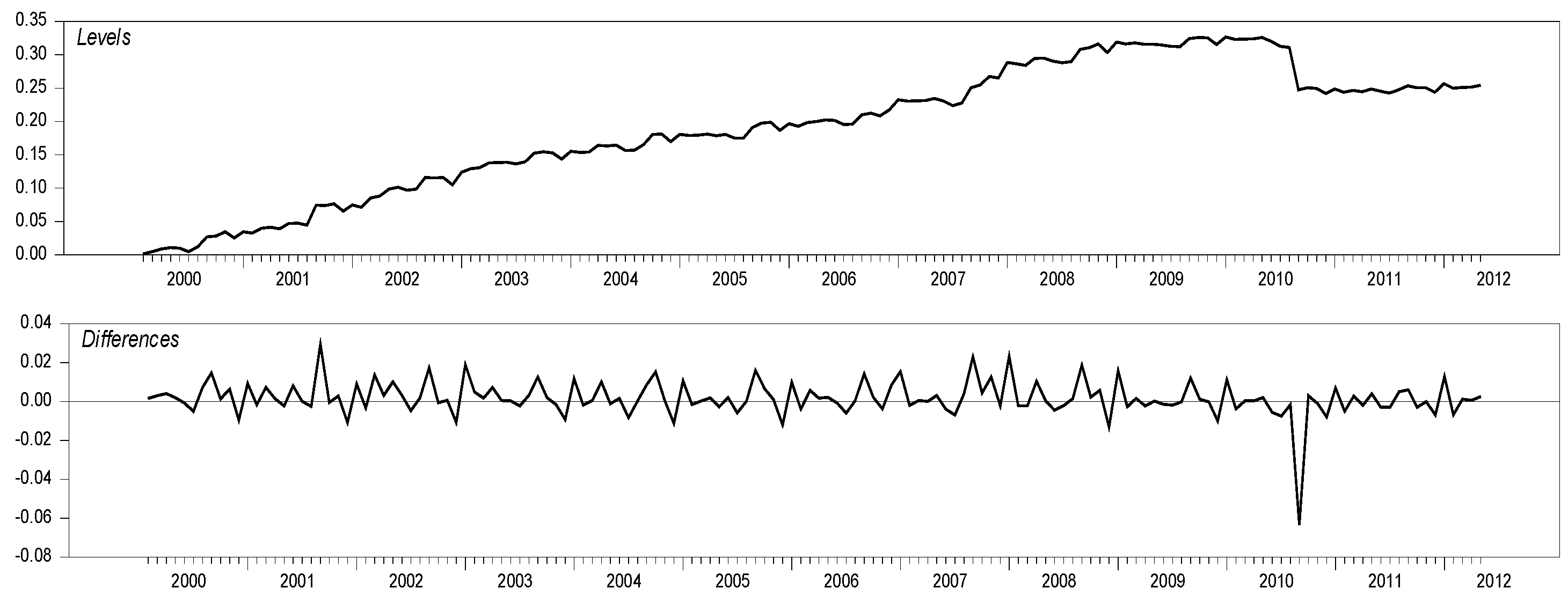
To understand the homogeneity of prices in long-run relationships in the tourism industry and to test H1, H2 and H3, we start with a cointegration analysis introduced by Johansen (1995); Juselius (2009, p. 217) and Hoover and Juselius (2015). A model is formulated with all the basic assumptions, with testable hypotheses about the model VAR. We developed the statistical VAR model in the way of Johansen (2012, 2019). The VAR model is created by the transformation of integrated nominal seasonal tourism prices into real ones. The latter suggests inspection of the data by the graphical analysis presented in Figure 1, Figure 2, Figure 3, Figure 4, Figure 5, Figure 6, Figure 7, Figure 8, Figure 9, Figure 10, Figure 11, Figure 12 and Figure 13 and Appendix C.

3.1. Descriptive Properties of Time-Series Data

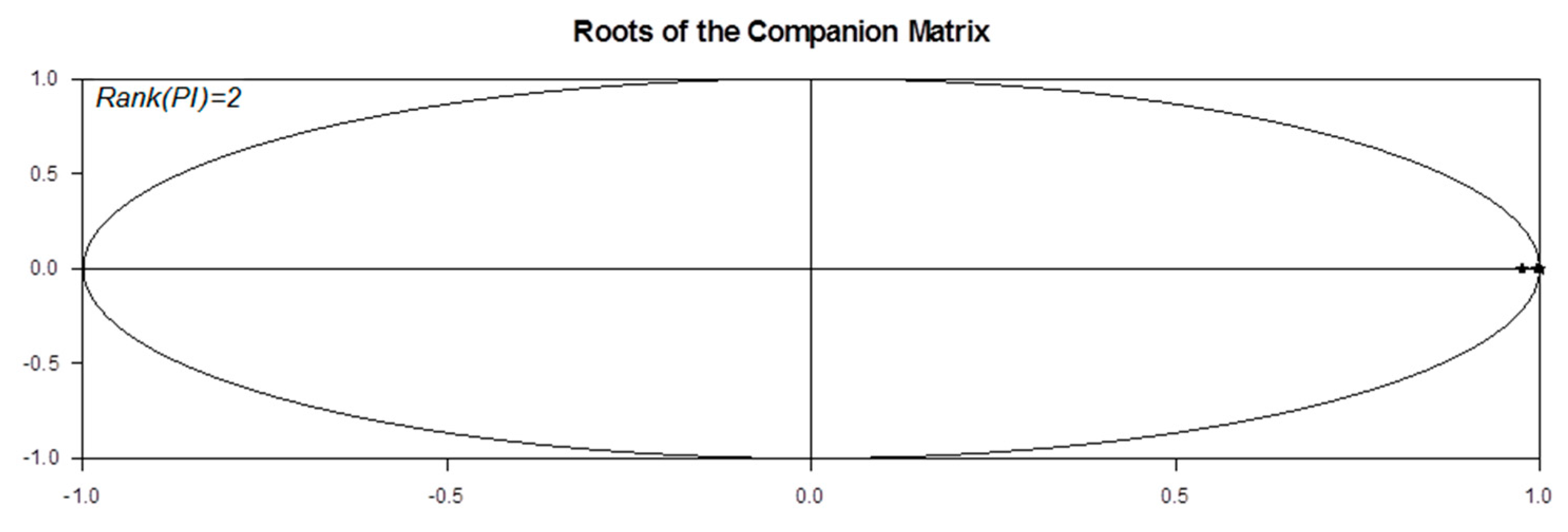
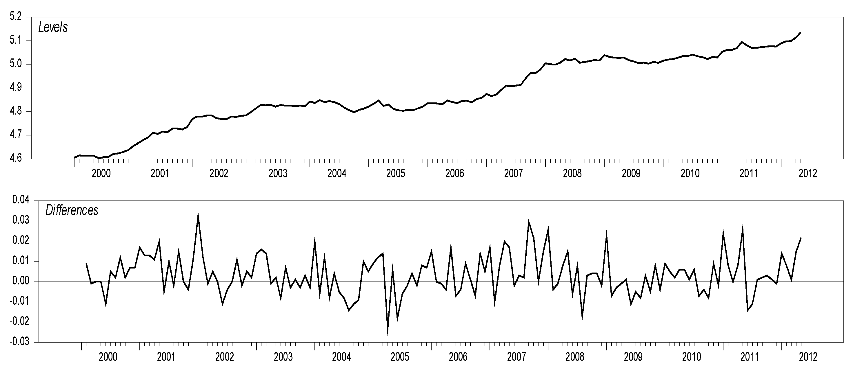
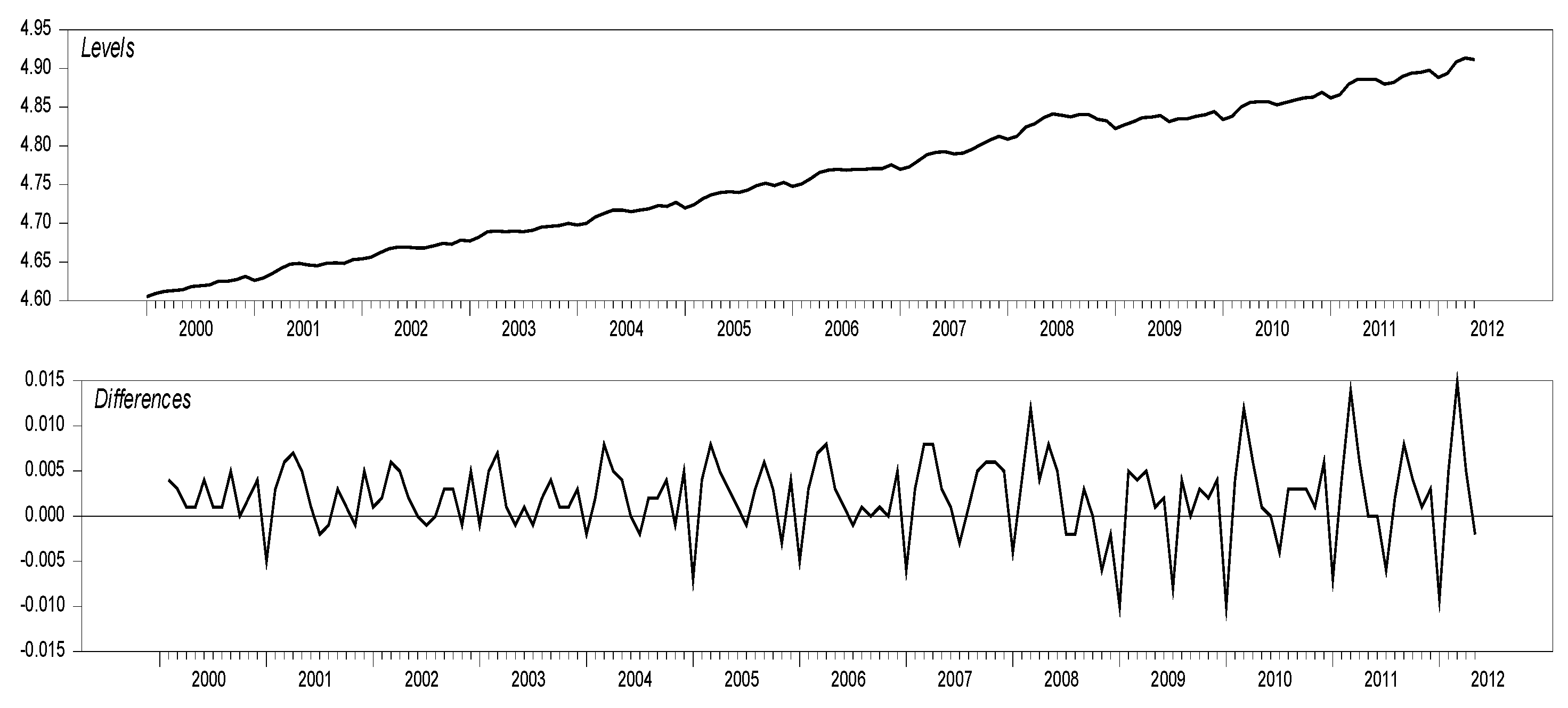
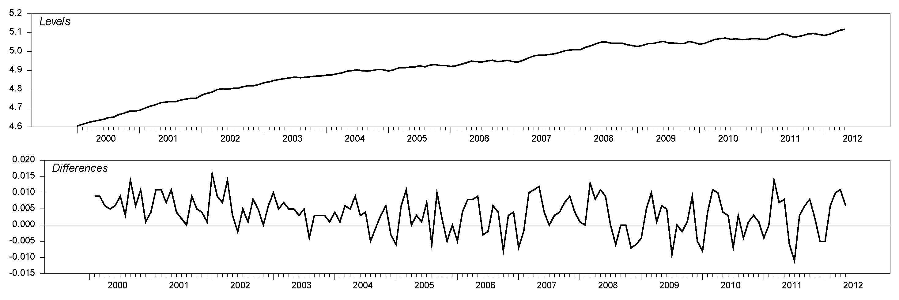
The testing hypotheses focus on hospitality industry prices in a cointegration relationship using seasonally unadjusted variables from the Statistical Office of the Republic of Slovenia (SURS) (https://pxweb.stat.si/sistat, accessed on 18 October 2021) and Eurostat (https://ec.europa.eu/eurostat/en/web/main/data/database, accessed on 18 October 2021). Figure 1 illustrates the increase in all empirical price indices in levels over the period starting in January 2000. The period from January 2000 to May 2012 includes cyclicity, both in terms of expansion and crisis. Time-series indices are for the consumer price index ( C P I t ) and other price indices used in time-series data analysis: the Slovenian food and beverages price index ( I F B t ), the Slovenian price index in the hospitality industry ( I P H I t ), the Eurozone price index in the hospitality industry ( I P H I E A t ), and the consumer price index in the Eurozone ( C P I E A t ). The constant base period indices are with January 2000 = 100. The stationary characteristics of the model to define roots need an apparent assumption of log-linearisation. The largest constant steady-states of the model were 1.000 and the lowest one 0.976. A root of 1.000 is in application identical to a unit root. Therefore, a root of 0.976 is nearly unity as a good source of persistency in the data (Figure 2). In addition, the tests for the data properties of each variable are presented in Appendix C (Table A3, Table A4 and Table A5), while necessary misspecification tests are presented in Table 1.
We present an approach that has not been used before to solve the problem of unit roots in the data and their impact on inference. By converting the data into stationary components using differentiation and cointegration (Juselius 2009), standard inference can be reapplied. Our goal is to develop the new econometric unit root theory for further analysis in modelling tourism prices with the conversion from nominal to real price time series without losing information in the data due to deflation or seasonal processing. As is known from theory, price time-series data are close to the second order of integration, as seen in Figure 3 (Chang 2000; Juselius 2015).
The inspection of plots yields the following noteworthy insights. First, all variables follow the same stochastic trend. Except for the C P I E A t , all other four time-series in the second differences can be I ( 1 ) . The stochastic trend is considered as an I ( 2 ) process, while the volatility of four variables could be more accurate than they are (Juselius 2009). The order of integration is known as how many times a time-series should be differenced to achieve stationary (Kivedal 2014, p. 53). We say that trend-adjusted prices are integrated of order two, or in shorthand notation P t ~ I ( 2 ) .
In addition, in Figure 4, Figure 5, Figure 6, Figure 7 and Figure 8, empirical time-series data in the sample have a linear trend, which describes that time-series are moving in a linear combination. Table 1 shows the properties of the time-series data used in a general VAR model. The number of observations for each of the variables is 149. The mean value is the smallest for the C P I E A t and the highest for the I P H I t (January 2000 = 100). The variable of the C P I t has a maximum value of 138.35. The distribution of price indices indicates the characteristics of the time-series data and the distribution of indices in terms of level, which are not similar to a normal distribution.

3.2. Misspecification Test of Data Used and Data Transformation

The statistical misspecification tests of the VAR model in Table 1 shows that the null hypothesis of residual normality without the presence of autocorrelation and heteroskedasticity (ARCH test) can be rejected for the model and some variables. Furthermore, the cross correlogram shows significant correlations between the errors, which are assumed to be independent. A diagnostic check detects explicit transgression of distribution. The main conclusion is that it is essential to specify the model further. However, the focus of the applied example that tests technical results of this theoretical research is on one country, i.e., Slovenia.
To observe the intelligent statistical nature of the data, we formulate a VAR model. After initial investigations1 (see Appendix A, Table A1), we conclude with a model with two lags and an unrestricted constant (Johansen 2012; Li and Bauer 2020). The model should find a correlational relationship among the time series. We detect a stochastic trend in the time-series data.
At this analysis point, one should consider the standard variables in empirical research with the time-series data for prices (Hoover and Juselius 2015). The analysis in tourism price modelling is based on converting nominal data to real data without losing information in the data by deflating or seasonal processing (Juselius 2015). Therefore, an additional formulation is obtained by taking logarithms but now specifying new variables. It is a logarithmic autoregressive transformation, where better insight into the variables is taken into account, e.g., it is much easier to define an expected range of values that lies outside the mean in the Δ X t than in the X t . We have transformed variables from nominal to real price indices as follows: the Slovenian price index in the hospitality industry:
( R P H t r = l o g ( I P H I t I P H I E A t ) ) ,
the Slovenian consumer price index:
( R P t r = l o g ( C P I t C P I E A t ) ) ,
and the Slovenian food and beverage price index:
( R F B P t r = l o g ( I F B t I P H I E A t ) ) ,
where symbol R indicate that the variable was created from nominal to real, r indicate real, t time-series variable and variables are at least I ( 1 ) ; X t r ~   I ( 1 ) . Therefore, we decided to use the logarithms transformed C P I E A t   and I P H I E A t by their past values:
( d P E A t 1 = l o g ( C P I E A t C P I E A t 1 ) ) ,   and
the price index in the hospitality industry in the Eurozone:
( d P H E A t 1 = l o g ( I P H I E A t I P H I E A t 1 ) ) ,
stationary in the first differences. Each of the time-series of price indices is at most ~ I ( 1 ) (Juselius 2009).
Hypothetical models postulate stability. Hoover and Juselius (2015) argue that there is no prospect of stable relationships in reality. Real variables are entirely analogous to the analytic design for computing a variable. The observables (nominal) are the variables that are collected. If the variables collected are to be valid, they should be analogous to the actual (real) variables. The inadequacy of such correspondence poses a methodological research problem that can be poker-faced. In this paper, we isolate a new economic unit root consonance to compensate for the absence of tourism variables. The latter is a price transformation from nominal to real prices, so the process is essentially empirical.
The formal multivariate misspecification test is used instead of the univariate Dickey-Fuller test (Juselius 2015; Cavaliere et al. 2015). The null hypothesis is that the model is precisely defined (Narayan 2003), but no alternative hypothesis exists.

3.3. Data Vector of Real Price Variables

Note that ( R P H t r d P H E A t 1 , , p ) ~ I ( 1 ) implies ( Δ I P H I t Δ I P H I E A t , , p ) , meaning long-term price homogeneity or cointegration among price indices. In this case, the stochastic trend in price indices can equally be measured by the stochastic trend in the growth of prices (Juselius 2009). Differenced variables of time-series ( d P H E A t 1 and d P E A t 1 ) looks very similar from a stochastic point of view. On this basis, it is assumed that three variables of price indices are I ( 2 ) in a convenient way to transform nominal price index data vector [ I F B t ,   I P H I t ,   C P I t ] into real price index vector   [ R F B P t r ,   R P H t r , R P t r ] as described in Equations (1)–(3). This data set is used in the empirical analysis to illustrate research and policy-relevant empirical results. The data vector of real price indices can be rewritten as:
[ r p h   r p   r f b p ] t T N r   [ d p e a   d p h e a ] t 1 T N r ,   T = 2000 : 1 , ,   2012 : 5 ; N = 149
where now data vector in real expressions can be used in further analysis. The newly proposed method is better than traditional methods in practice using variables integrated of the first order. In addition, the variable line crosses the mean line several times, which shows that the variable is normally distributed with low variance in time-series residuals.

3.4. Robustness Testing of Lagged Comparative Analysis

We included the main Slovenian guests’ incoming destination countries that influence Slovenian tourism. These include Austria, Italy, Germany, and Croatia, The variables are identical to those for Slovenia, and the results are presented in Appendix B.
Asymptotic distribution tests were performed in an extended comparative time-series of the Eurozone (Appendix C). Croatia will adopt the euro in 2023, while the exchange rate has remained since 2012. According to European Central Bank, the average exchange rate was 7.525 Croatian kunas for one euro (ECB 2021). The Exchange-rate mechanism (ERMII) central rate has been fixed at 7.5345 Croatian kunas for one euro since 10 July 2020 (ECB 2020). Therefore, the subsequent data vector of robust tests represents the economic expansion period of the five countries from 2012 to 2020. The results are presented in Appendix C.
Overall, the panel case study demonstrates the robustness of the original analysis in the case of Slovenia. Moreover, the picture of the comparability of the methodology is presented. The usual misspecification tests were not used in the first part of the study, i.e., ADF and AIC tests. On the other hand, we have shown the technical application of the more robust Multi Auto-Regressive Conditional Heteroscedasticity (ARCH) tests and the normality test Jarque-Bera. This research is an extension of the transmission of prices within the Eurozone.

4. Econometric Results

4.1. Statistical VAR Model

An additional need is for the correctly defined unrestricted VAR model, which is an appropriate conclusion of the covariances of the data (Hendry and Mizon 1990; Juselius 2009, p. 32; 2015; Polito and Wickens 2012). Therefore, it can represent the reality consistent with the described theoretical model.
The hypothetical k -th order VAR model is:
X t = μ 0 + Π 1 · X t + 1 + + Π k · X t k + ε t ,   t = 1 , T ,
where ε t is N I p ( 0 , Ω ) and X 0 , ,   X k + 1   are expected to be fixed. Thereby, surprisingly when the variables X t are firmly time-dependent, the conditional process ( X t | X t 1 0 ) is independent and ordinary least squares estimates of { Π 1 ,   , Π k ,   μ 0 ,   Ω } are Maximum Likelihood estimates (Hendry and Mizon 1990).
Within the VAR model, the cointegration hypothesis can be formulated as a reduced rank restriction on the Π matrix in Equation (7). The VAR(2) model is the following:
Π X t = 0.006 0.006 0.009 0.009 0.054 0.010 0.028 0.061 0.007 0.003 0.004 0.003 0.004 0.005 0.001         0.216 0.508 0.001 0.233 0.562 0.006 1.236 0.262 0.004 0.883 0.089 0.002 0.047 0.852 0.002 ,   and
if X t ~ I ( 0 ) , then Δ X t ~ I ( 0 ) implying that Π cannot have the full rank as this would lead to a logical inconsistency. In this case, Π can be obtained by considering Π = I as a simple full matrix.

4.2. Deterministic Components

An introduction of the full VAR model is our next step in the modelling approach where we are assuming that r = 1 . This means that there is only one stationary relationship among five analysed price time-series, the Slovenian hospitality industry price indices relationship. Using our data on price indices α 11 = 0.006 and β 1 = [ 2.6 , 10.2 , 2.7 , 581.1 , 86.9 , 0.3 ] , we can reproduce the first raw of Π as α 11 β 1 . We can now rewrite the cointegrated VAR model:
[ R H P t R P t R F B P t d P E A t 1 d P H E A t 1 ] = [ 0.006 α 21 α 31 α 41 α 51 ] [ { 2.6 · R P H t 10.2 · R P t + 2.7 · R F B P t + + 581.1 · d P E A t 1 86.9 · d P H E A t 1 } i ] + [ μ 1 μ 2 μ 3 μ 4 μ 5 ] + [ ε 1 , t ε 2 , t ε 3 , t ε 4 , t 1 ε 5 , t 1 ] ,  
if, for simplicity, we assume that Γ 1 = 0 .
It is easier to understand an expected range of values that lies outside the mean in the Δ X t than in the X t , and the visual test presented in Figure 9, Figure 10, Figure 11, Figure 12 and Figure 13 is performed. Additionally, the inspection of the results on the unrestricted VAR(2) model for the data showed high R F B P t in months January 2002 ( D p 021 t ), September 2007 ( D p 079 t ), and November 2007 ( D p 0711 t ), which is caused by the significant monthly increases. The first tentative conclusion for the unrestricted model VAR(2) is a policy shift, for example, with a permanent or impulse dummy (differentiated variable) that can be generated by generating the differentiated process. Almost all policy changes in our model are permanent. This is true not only for high food price indices but also for the seasonal declines in the R H P t in September 2001 ( D p 019 t ), October 2004 ( D p 0410 t ), and in September 2010 ( D s 109 t ). This can be linked to the attacks of 11 September 2001 and Slovenia’s accession to the EU in 2004. In the last quarter of 2010, the R H P t fell rapidly by 13.02% on a monthly basis. D s 1009 t is a mean shift dummy or blip (in differences) variable. Our last permanent dummy was in December 2006 ( D p 0612 t ) on the month before Slovenia adopted the euro. Testing the normality of structural breaks (dummies) included in Equation (11) are presented at the bottom part of Table 2.
Utilising dummies to capture for remarkable mean-shifts, permanent blips, and transitory shocks, the CVAR model from Equation (A7) (Appendix D) is reformulated as:
Δ X t = Γ 1 · Δ X t 1 + α · β · X t 1 + + ϕ p · D p , t + ϕ s · D s , t + μ 0 + ε t ,
where ε t ~ N I ( 0 , Ω ) , t = 1 , T , D p , t is a d 1 × 1 vector of permanent blip dummy variables ( , 0 , 0 , 1 , 0 , 0 , ) , and D s , t is a d 2 × 2 vector of mean-shift dummy variables ( , 0 , 0 , 0 , 1 , 1 , 1 , ) (Juselius 2009). We can now re-estimate the CVAR model:
Δ x t = Γ 1 · Δ x t 1 + α · β · x t 1 + ϕ p . 1 · D p 019 t + ϕ p . 2 · D p 021 t + ϕ p . 3 · D p 0410 t + ϕ p . 4 · D p 079 t + ϕ p . 5 · D p 0711 t + ϕ p . 6 · D p 0612 t + ϕ s . 7 · D s 109 t + γ 0 + ε t .
We improve the possessions of the calculated VAR(2) model with dummies in contrast to the unrestricted VAR(2) model (Kivedal 2014, p. 49). The VAR(2) model does not contain autocorrelations and the ARCH(2) effect for conditional heteroscedasticity. Skewnesses and kurtosis lead to the normal distribution of all variables. Lag Reduction Tests (LR) for k = 2 is applied2. The empirical outcomes of the misspecification test for the VAR(2) model are presented in Table 2. The model VAR(2) is now well defined for the errors to be normally distributed and for the test statistics to be consistent with chi-squared ( χ 2 ) Distribution. The lag length is susceptible to the misspecification test. This is especially true for the level shifts in the model because the VAR(2) model specifications and the determination of the lag length belong together.

4.3. Cointegration Rank

In the applied Johansen test or trace test, the LR test for the cointegration rank, all exogenous variables, e.g., deterministic components, are included in the VAR model (8). In the empirical analysis, the constant term is restricted to the cointegration relations. Thus, there are no included trends in the levels, but there are included non-zero means in the cointegration relations. We restrict the VAR model, meaning that the five price index variables in the VAR model have r cointegration relations and n r common stochastic trends (Juselius 2009). We estimated the VAR model for r = 1 , , 5 . We consider the LR trace test of the cointegration rank. We have found out the rank of three ( r = 3 ) (Table 2), with a trace test statistic, where p -value is 0.850 . Moreover, r = 2 is with p -value of 0.000 of the trace test. The choice of r = 3 is supported by the finding of three roots close to one, of which the largest were 0.998 and the second two 0.956.
From the α vector (Table 3), each of the price variables is significantly adjusting to the long-run equilibrium given by the first cointegration relation except for the d P H E A t 1 . In the second relation, only the R F B P t does not correspond to the long-run equilibrium. In the third cointegration relation, only   the   d P E A t 1 and d P H E A t 1 are significantly adjusted to the long-run equilibrium. The β vector can be normalised on any of the price variables. Note that when the R P H t in β is normalised, the adjustment coefficient for the R P H t in α is equal to the first row.
The final parsimonious VAR model describes regularities in the data without suppressing any relevant information. More specifically, by integrating differenced and cointegrated data, the CVAR model suggests a conventional way of analysing price time-series data as short-run adjustments around moving long-run equilibrium. The CVAR model gives the data a rich context to speak freely (Hoover and Juselius 2015). For the model, estimation is used in the I ( 1 ) framework of the CVAR model. The three cointegration relationships and the two stochastic trends are performed.

4.4. Combined Effects in Π Matrix

We aim to formulate hypotheses tests on the cointegration vectors. We consider the test for the long-run selection of a price variable, i.e., the variable can be removed from the cointegration space. We have estimated the VAR model with a level shift in D s 109 t and manually included the first difference with one lag and imposed r = 3 . In addition, we consider the Π matrix. If a variable in the cointegration relations can be omitted, the coefficients in the respective column of the matrix must be insignificant. From the Π matrix, there are no clear signs that any of the variables can be omitted from the cointegration relations, except for the R P H t   variable. Now, we design the Π matrix for the hypothesis that the first variable can be excluded from the cointegration relations where s is the number of free parameters. We restrict one of the p = 7 (5 variables, shift, and a constant) to obtain s = 6 . For a r = 3 , none of the five variables or the restricted level shift can be excluded from the cointegration relations, except for the R P H t . But we have decided that the variable R P H t will stay in the cointegration space to test the long-run relationship on this variable in the cointegration space. Moreover, when the cointegration rank of r = 1 is chosen, we can exclude the R P H t , d P E A t 1 . So the single cointegration relation in the VAR model is a relation between the consumer price indices for inflation rates and the food and beverage price indices.

4.5. Test of Stationarity

If price variable i is stationary around a constant mean with a D s 109 t , then one of the cointegration relations must be given by a linear combination of variable i , the constant term and the D s 109 t . When testing for stationarity of variable i we restrict one of the cointegration relations to variable i , the constant term and the D s 109 t , while leaving the other cointegration relations unrestricted. For r = 3 , we restrict one relation while keeping the other unrestricted. For r = 3 , the automatic tests of CATS for RATS (OxMetrics) are equal to the manually calculated tests. For r = 2 (and r = 1 ) none of the variables is stationary by themselves. Note that the choice of the cointegration rank matters for the stationarity of the single variables. For r = 3 the d P E A t 1 and the d P H E A t 1 become borderline stationary, implying that a linear combination of d P E A t 1 and the d P H E A t 1 , the constant term and the D s 109 t can yield the third cointegration relation.

4.6. Hypotheses Testing

To test the relation for H1:
β 1 · C * · x t = R P H t d P H E A t 1 d P E A t 1 ,
the linear combination corresponds to a stationary spread in price indices, which means that the price indices converge in the long term. We can test if the linear combination is stationary around a constant with D s 109 t by formulating the hypothesis in terms of the design matrix H [ 1   0   0 1 1   0   0 ] . We have ( s 1 = 3 ) free parameters in the first cointegration relation as we impose homogeneity restrictions between the price indices. We estimate the VAR model and impose r = 3 . We reject the hypothesis of a stationary spread in price indices at p -value = 0.003 . If we restrict each of the price indices with the included constant, we cannot reject the hypothesis of stationary.
To test the relation for H2:
β 2 · C * · x t = R P H t R F B P t ,
is estimated the VAR model and imposed restriction r = 3 . We reject the hypothesis of a stationary price index spread at p -value = 0.044 . In addition, we restrict each variable with the constant. In this case, we cannot reject the hypothesis of stationary cost-push transmission of the Slovenian food and beverages price indices on the Slovenian price indices in the hospitality industry.
To test the relation for H3:
β 3 · C * · x t = R P t d P E A t 1 ,
is estimated the VAR model and imposed restriction r = 3 . We reject the hypothesis of a stationary spread in the price indices at p -value =   0.003 . If we impose restrictions also on the dummy variable, we cannot reject the hypothesis of stationary. This procedure implies the convergence among the price indices.
Relying on the H1, H2 and H3 test results, the following joint hypothesis on the full cointegration structure is tested simultaneously:
4 = β { H 1 φ 1 ,   H 2 φ 2 , H 3 φ 3 } ,
where H1 corresponds to a homogeneous relation between the Slovenian price indices in the hospitality industry, C P I E A t , and the eurozone price indices in the hospitality industry, H2 corresponds to a relation between the I F B t and the I P H I t , and H3 corresponds to the C P I t . and the C P I E A t .

4.7. Long-Term Identification

The final step is to introduce the theory of consistent restrictions. Juselius (2009) discussed that the VAR model for inflation is based on the assumption. For the 4 . in Equation (22), the nineteen over-identifying restrictions were tested using the LR test procedure in Johansen (2012) and recognised with a p -value = 0.732 . The empirical results are presented in Table 3. Each of the β coefficients is strongly significant, indicating that the structure of the joint hypothesis 4 is formally and empirically identified.
The first vector is given by:
d P E A t 1 = 0.004 · R P H t + 0.397 · d P H E A t 0.002 + s t a t . e r r o r , and
C P I E A t is negatively associated with the Slovenian price indices in the hospitality industry (an imported deflation effect) and positively associated with the price indices in the Eurozone price indices in the hospitality industry. The constant term shows that the hospitality industry price indices, on average, are lower than the indicated value as given by the determinants. As can be seen, the normalisation on β cannot be made on the R P H t , while the R P H t should be excluded, as suggested by the misspecification test and Π matrix. Similar findings have been made by Bianchi and Chen (2020). They did not find that long-term cycles are time-varying for Switzerland.
Moreover, by normalising the β coefficient on the variable of the Slovenian price indices in the hospitality industry β ˜ 1 = ( 1   0   0   1   1   0   1 ) in a long-run relationship in the first cointegration equation, we defined the consumer price indices in the Eurozone. They are being driven by the eurozone price indices in the hospitality industry. This conclusion confirmed that we could not reject the null hypothesis of the restrictions on β ˜ 1 = ( 1   0   0   1   1   0   1 ) with a p -value = 0.810 . In the cointegration relation, it is assumed that when the Slovenian price indices in the hospitality industry rise, then statistically significantly decline in the eurozone price indices in the hospitality industry occur. This implies the convergence among the lower Slovenian prices in the hospitality industry and the higher eurozone price indices in the hospitality industry.
The second cointegrating relationship is given by:
d P E A t 1 = 0.006 · R P H t + 0.004 · R P t + 0.003 + s t a t . e r r o r , and
represents the C P I E A t . The interpretation is that the C P I E A t is positively correlated with the C P I t and negatively correlated with the Slovenian price indices in the hospitality industry. The constant term shows that the C P I E A t on average, they are higher than the implied value.
The third vector is a function of the Eurozone price indices in the hospitality industry and can be written as:
d P H E A t 1 = 0.005 · R F B P t + 0.866 · d P E A t 1 0.001 · D s 109 t + s t a t . e r r o r . ,
with the following interpretation: the Eurozone price indices in the hospitality industry are positively associated with the Slovenian food and beverage price indices and negatively associated with the consumer price indices in the Eurozone. The shift dummy is consistent with a slight decrease in the Eurozone price indices in the hospitality industry after the economic crisis. The results confirmed the stationarity of the shift dummy.
To sum up, in the long run, the consumer price indices in the Eurozone have a positive impact on the price indices in Eurozone price indices in the hospitality industry (16). The consumer price indices in the Eurozone positively impact the Slovenian consumer price indices (H1), but the opposite is true for the impact on the Slovenian price indices in the hospitality industry (17). Moreover, the Eurozone price indices in the hospitality industry have a positive impact on the Slovenian food and beverages price indices (18). Our findings do not confirm the H2. In addition, the Eurozone price indices in the hospitality sector fell in September 2010 following the economic crisis (18).
The empirical results support the theoretical description of inflation, price transmissions and price rise in the Eurozone (Bakucs et al. 2012; Hoover and Juselius 2015).

5. Discussion

5.1. Formal Discussion

An intensive analysis of the dependence on the cointegrated tourism price structures among tourism markets is essential for hotel and tourism experts, policymakers, and practitioners. Indeed, most contemporary literature on tourism price linkages has applied approaches to detecting demand and supply factors, co-movements or correlations without considering the normality of the statistical model and further empirical i.i.d. model (Arnastauskaitė et al. 2021). Nonetheless, most previous empirical research has neglected the dependence on the composition (high correlation) among multiple time-series variables from a (spatial) interaction modelling perspective (Dritsakis 2004).
This paper presents a dynamic time-series data model with the nominal vs. real tourism prices, cointegrating the VAR(2) type model (Kongsted 2005). This technical approach is developed and applied for estimating well defined statistical and empirical models among tourism markets. The model is partly extended to the VAR model previously developed by Juselius (2009, 2015, 2021) and then compared to the CVAR estimation developed by Johansen (2012, 2019) and Johansen and Tabor (2017).
The new theoretical and applied approach to the comparison of real-tourism price variables is introduced. The paper follows previous theoretical considerations of Hoover and Juselius (2015); Juselius (2015); Johansen and Nielsen (2018) and Schild and Schweikert (2019). An endeavour of the research contributes to the econometric theory on skew-normal price time-series distributions (Trafimow 2019).
Prices are found to be integrated into order two. Therefore, we decided, first, to use the natural logarithm-transformed consumer prices in the Eurozone and the eurozone price indices in the hospitality industry. This transformation leads to the time-series variables integrated of order one. Second, the Slovenian consumer prices in the current month t are divided by the previous month t 1 value of the consumer prices in the Eurozone. The last step was creating the Slovenian prices in the hospitality industry and the Slovenian food and beverage prices in the current month t to be integrated into order one by dividing both variables by the previous month t 1 values of the eurozone price indices in the hospitality industry.
The formal misspecification tests of transformed real data vector have confirmed that the VAR model does not contain autocorrelations and heteroskedasticity in the residuals. Therefore, the normality tests were assumed to be based on skewness and kurtosis of the standardised estimated errors. The null hypothesis of normality cannot be rejected ( p = 0.315 ). Experimenting with the stability of the VAR model derives to the conclusion that there are several permanent dummies needed, where the most obvious one, by using the visual inspection of the VAR model, is a mean shift dummy for September 2010 (Figure 6). This dummy is also statistically significant. It is used to normalise the cointegration equations. Other permanent dummies are just involved in the VAR model but not in the cointegration relations.
The unrestricted VAR model has two lags and a rank of three, deriving eigenvalues by using the trace or Johansen test. In the restricted VAR model, there are non-weakly exogenous variables. In that sense, all five included variables in the VAR model are endogenous.

5.2. User-Friendly Discussion on Technical Analysis

This rare study deals technically with normalities in a time-series (Kongsted 2005; Juselius 2021; Vougas 2021). Econometricians (Johansen 2019) usually define and prove a purely theoretical treatment of this system (Archontakis and Mosconi 2021; Franchi and Paruolo 2021). In addition, this study contributes to a step-by-step process to show the time-series technicalities, similar to Pacifico (2021), on volatilities. The dependencies between variables and the data errors are often discussed, but the random walk within time-series is rarely discussed in technical solutions. Moreover, the distribution of shocks due to the lag length or transformation of variables, such as de-sesonalization, is often omitted.
In contrast, we try to show how to deal with these collinearities in a technical and user-friendly way; nevertheless, omitting the test of normalities is a scary time-series error. Therefore, the importance of misspecification tests for multi-variable modelling is technically presented in this paper; for example, standard tests such as the Augmented Dickey-Fuller test (ADF), Kwiatkowski–Phillips–Schmidt–Shin (KPSS) and others are placed in Appendices. We want to highlight the following essential steps:
  • Think about the problem, not just from theory but from real life;
  • Define hypothesis and methodology, although we discuss only the applied time-series;
  • Identify strategically important variables;
  • Test the variables and find the normalities in the variables. Do not proceed until a solution is found, as technically presented in this study for price variables. This step may take the longest time;
  • When normalities are found, and the correlation between them is low, the random walk is solved. One can proceed with the methodology that determines the results;
  • The results obtained can now be discussed;
  • Test the model for all misspecification cheques. If it is not acceptable, go back to the variables. Something is probably wrong in this step;
  • If the normalities are found in the model, which usually takes some time, you can continue to the next step;
  • The results, including the predictions, can be presented.
So if any of the above steps are omitted, the results can be biased and need re-sampling (Pollock 2020). Therefore, the results of many economic papers could be wrong because they are based on bivariate test solutions, which are usually only a starting point, including visual tests. This step-by-step technical procedure can greatly interest other researchers who encounter significant problems in dealing with time-series (Hudecová et al. 2021). Nevertheless, our conceptual contribution is discussed in a transformation from nominal to real problems in price variables, in our case, tourism prices, which solve misspecifications (Harvey et al. 2012; Desgagné and de Micheaux 2018). Tourism prices are one of the markets with large fluctuations and therefore contain policy and other management information. Overall, Appendix B shows a comparative example of the leading Slovenian guest incoming destinations in the Alps Adriatic part of the Eurozone, omitting the transformation from nominal to real values but observing the transmission.

6. Conclusions

6.1. Novelty for Theory

This paper provides a cointegrated vector autoregressive model to study tourism prices in the long run. The main theoretical contributions are (1) a developed integer for testing non-normality for time-series, and (2) the long-run cointegration spread of tourism prices. This paper contributes to the study of the creation of spatial integrated nominal (observational) tourism prices into real (true) ones across national economies, supporting the most advanced technical analysis. More specifically, considering the previous empirical studies, our study contributes to the field in several ways.
First, our suggested VAR(2) model is positioned above the most of previous ones to reveal the dependence structure of high-dimensional tourism time-series data because the model reflects on serial autocorrelations across error units simultaneously rather than separately. The applied weak stationary experiments evaluate the performance and robustness of the derived nominal vs. real estimator of our proposed VAR(2) model. In addition, our results clearly show that error correlations are better modelled jointly in terms of the real data vector-matrix than specified in the previous studies.
Second, we confirmed that the absolute values study tourism prices and the relative values determined by stochastic and deterministic volatilities. Hence, differently from the previous empirical studies, we use the relative values of the estimated conditional variance to construct the exogenous variables. It is reasonable to define tourism price volatility on each data frequency (in our case, the month) and then regard these created dummy variables, which additionally perform exogenous explanatory variables because tourism prices might be affected by seasonal stochastic volatilities. To the best of our knowledge, this article is the first to incorporate nominal vs. real tourism prices without losing any information borne by price into the definition of the real data vector. Additionally, our model compared to previous ones does not support deflating procedures.
Finally, our suggested spatial consolidated CVAR model is more straightforward and provides a more precise visualisation of the dependence structure between explanatory variables, e.g., tourism price indices. The proposed model is up to date, empirically well defined, and it is user friendly. Our results also confirm the findings of other applied studies that the tourism prices are near the second-order of integration and consumer price index is integrated of the first order.

6.2. Implications for Policymakers in Tourism

The main result of this empirical analysis confirms the importance of Eurozone prices for its member state hospitality industry prices. The hypotheses testing confirmed cointegrated relations between the national and Eurozone prices and vice-versa. On the other hand, input costs in the hospitality industry are not in a linear cointegration spread. To sum up, Slovenia’s tourism and hospitality industry prices are purely internationally driven other than seasonally driven, and accomplished due to a stochastic shock.
Empirical results confirm that the tourism prices in Slovenia in the studied period are negatively correlated with the consumer prices in the Eurozone in the previous period and are positively correlated with the tourism price indices in the Eurozone. The reason can be described by the adjustments and convergences of the Slovenian prices as the new member state of the EU and Eurozone to the enlarged EU borderless single market and Euro area.

6.3. Limitations of the Research and Future Research Perspectives

Among the main limitations of the study is that other competing tourism markets in the Eurozone and its time-series models were not considered, as well as modifications in the spatial and temporal dependence structures.
Among issues for further research, one is to apply the I ( 2 ) VAR model with more extended period time-series data to increase the degrees of freedom as proposed by Di Iorio et al. (2016). Furthermore, the Cavaliere et al. (2015) bootstrap test can be applied. This insert is to solve the inference problem where the null hypothesis is imposed on the bootstrap sample. The research could be extended by the VECM diagnosis proposed by Barigozzi et al. (2020) or by panel cointegration.
Among the empirical model applications, it is recommended to compare and analyse national prices in the hospitality industry for some other countries in the Eurozone to gain new knowledge on spatial market integration and price transmission and causalities between the eurozone price indices in the hospitality industry and the national ones. Finally, a procedure could also be applied to transform existing data with I ( 1 ) VAR to the short-run empirical research model of the eurozone price indices in the hospitality industry. This finding would give new evidence on real seasonal price implications.
While supply and demand determine prices and tourism uses public services, the integration of the Internet of Things (Lewis 2021), intelligent transportation (Taylor 2021), computational thinking (Konecny et al. 2021), Big Data and self-driving cars (Mitchell 2021), and chairs in hotels (Gričar 2014) are the future of tourism development. Therefore, artificial neural networks (Gricar et al. 2021) are an essential component of future tourism and hospitality development, as well as technology in research on smart, sustainable cities (Townsend 2021) and destination management (Harris 2021).

Author Contributions

Conceptualisation, S.G.; methodology, S.G.; software, S.G.; validation, S.G. and Š.B.; formal analysis, S.G.; investigation, S.G.; resources, S.G.; data curation, S.G.; writing—original draft preparation, S.G.; writing—review and editing, Š.B. and S.G.; visualisation, Š.B. and S.G.; supervision, Š.B.; project administration, S.G.; funding acquisition, S.G. and Š.B. All authors have read and agreed to the published version of the manuscript.

Funding

This research received no external funding.

Institutional Review Board Statement

Not applicable.

Informed Consent Statement

Not applicable.

Data Availability Statement

The data is in the public domain, and the relevant sources are cited in the text.

Acknowledgments

We are grateful for the comments of the Editor-in-Chief and guest editors. We thank three anonymous reviewers for their rigorous and detailed comments that improved the paper.

Conflicts of Interest

The authors declare no conflict of interest.

Appendix A

Table A1. The unit roots of the VAR(3) model.
The RootsRealModulus
root 11.001.00
root 21.001.00
root 30.880.88
root 4–0.480.48
root 50.110.40
root 60.110.40
root 70.400.40
root 8–0.090.09
root 90.020.09
root 100.020.09

Appendix B

The integration I ( d ) of time-series variables for Slovenia for the initial data vector (2000–2012) are presented in Table A2.
Table A2. The unit root tests—the integration I ( d ) (base period January 2000), data vector 2000 to 2012.
Unit Root TestsCPICPIEAIPHIIPHIEAIFB
ADF (levels)4.645.583.214.232.06
ADF ( I ( 1 ) )–4.76 ***–6.12 ***–5.37 ***–7.50 ***–5.04 ***
Note. IPHI—Slovenian price index in the hospitality industry, CPI—consumer price index in Slovenia, CPIEA—consumer price index in the Eurozone, IPHIEA—Eurozone price index in the hospitality industry, IFB—Slovenian food and beverages price index. ***: significance at 1% level.

Appendix C

Asymptotic distribution tests of comparative analysis for Austria, Croatia, Germany, Italy and Slovenia for subsequent data vector (2012–2020) are presented in Figure A1, Figure A2 and Figure A3 and in Table A3, Table A4 and Table A5. Therefore, the results section contributes to this extension on the transmission of prices within the Euro zone.
Note. The data source for all Figures in Appendix C is Eurostat (https://ec.europa.eu/eurostat/en/web/main/data/database, accessed on 18 October 2021).
Figure A1. (a) Distribution of consumer price indices for Austria, Croatia, Germany, Italy, and Slovenia; (b) Distribution of I ( 1 ) Consumer price indices for Austria, Croatia, Germany, Italy, and Slovenia. Note. CPI—Consumer price index; EU—Eurozone; D—Germany, HR—Croatia, I—Italy, A—Austria, SI—Slovenia. Data vector January 2012 to March 2020 (expansion period); d— I ( 1 ) .
Jrfm 14 00517 g0a1
Figure A2. (a) Distribution of food and beverages price indices for Austria, Croatia, Germany, Italy, and Slovenia; (b) Distribution of I ( 1 ) food and beverages price indices for Austria, Croatia, Germany, Italy, and Slovenia. Note. IFB—Food and beverages price index; EU—Eurozone; D—Germany, HR—Croatia, I—Italy, A—Austria, SI—Slovenia. Data vector January 2012 to March 2020 (expansion period); d— I ( 1 ) .
Jrfm 14 00517 g0a2
Figure A3. (a) Distribution of price indices in the hospitality industry for Austria, Croatia, Germany, Italy, and Slovenia; (b) Distribution of I ( 1 ) price indices in the hospitality industry for Austria, Croatia, Germany, Italy, and Slovenia. Note. IPHI—Price index in the hospitality industry; EU—Eurozone; D—Germany, HR—Croatia, I—Italy, A—Austria, and SI—Slovenia. Data vector January 2012 to March 2020 (expansion period); d— I ( 1 ) .
Jrfm 14 00517 g0a3
Table A3. Descriptive statistics of consumer price indices (base 2015), data vector 2012–2020.
Descriptive StatisticsEUDHRIASI
Mean (levels)103.3286.1391.6398.0587.88125.70
N999999999999
Skewness   ( I ( 1 ) )–0.58–0.27–0.29–0.16–0.33–0.31
Kurtosis ( I ( 1 ) )–0.44–1.02–0.68–0.93–0.94–0.21
Normality   test   ( I ( 1 ) )4.09 *3.001.872.703.191.23
Note. Abbreviations are explained under Figure A1, Figure A2 and Figure A3. *: significance at 10% level.
Table A4. Descriptive statistics of food and beverages price indices (base 2015), data vector 2012–2020.
Descriptive StatisticsEUDHRIASI
Mean (levels)100.5696.56134.0781.5463.52113.02
N999999999999
Skewness   ( I ( 1 ) )2.022.571.591.191.262.62
Kurtosis ( I ( 1 ) )4.047.232.971.342.467.23
Normality   test   ( I ( 1 ) )133.19 ***320.81 ***75.18 ***30.39 ***50.54 ***325.49 ***
Note. Abbreviations are explained under Figure A1, Figure A2 and Figure A3. ***: significance at 1% level.
Table A5. Descriptive statistics of price indices in the hospitality industry (base 2015), data vector 2012–2020.
Descriptive StatisticsEUDHRIASI
Mean (levels)78.8639.7768.6673.3689.63111.90
N999999999999
Skewness   ( I ( 1 ) )2.352.252.371.793.082.73
Kurtosis ( I ( 1 ) )5.074.985.112.589.667.11
Normality   test   ( I ( 1 ) )97.54 ***89.52 ***108.70 ***19.15 ***709.33 ***283.73 ***
Note. Abbreviations are explained under Figure A1, Figure A2 and Figure A3. ***: significance at 1% level.

Appendix D

We start with the general VAR model used for data analysis. The VAR model with a constant term and two lags for a n dimensional process of a variable X t is given by Equation (A1)
H r :   Δ X t = α · β X t 1 + Γ · Δ X t 1 + μ + ε t ,
where white noise process
  ε t = x t μ t
is a difference between the conditional mean μ t and the actual realisation X t , which is normally independent N I p ( 0 , Ω ) , t = 1 , T , ( α ,   β ) are n × r matrices, r is a cointegration rank, X t 1 are past values of the variable, Δ X t is the first difference of the variable X t , μ is a mean vector for all periods T , and Γ is a covariance matrix (Narayan 2003; Johansen 2012, p. 51; 2019).
We can talk about cointegration when the variables are not in a correlation (Johansen 2012, p. 50). VAR model consists of a transformation of (time unchanged) covariances of the time-series information. Note that the values X t 1 and X 0 are needed as initial values in order to be able to generate the process recursively. Johansen (2012, p. 51) shows that under defined polynomial and further regularity conditions, the solution is nonstationary differences, and including matrix C it follows that X t is nonstationary with linear trend C · μ · t , and Δ X t is stationary. Matrix C satisfies β · C = 0 and C · α = 0 , and C i * are functions of α ,   β and Γ . Moreover,
β · X t = i = 0 β · C i * · ( ε t i + μ )
is also stationary, that X t is cointegrated with r cointegrating relations β and disequilibrium error
β · X t E · ( β · X t ) ,
where E is vector process of β · X t and i is a diagonal element. Additionally, X i has n r common stochastic trends, α · i = 1 t · ε i , where orthogonal complements α is p × ( n r ) of full rank and α · α = 0 , where α is the whole α matrix (Johansen 2012, p. 49; 2019).
The decision of lag length may follow the residuals, which are close to being i.i.d. Therefore, we first determine the lag length, and second, we need to find the cointegration rank and estimate and interpret the cointegrating relation. Finally, we need to clarify the model by testing coefficients α and β to zero (Gjelsvik et al. 2020; Juselius 2009).
We present the cointegrated VAR (CVAR) model (Kivedal 2014) applied to analyses of the tourism (Ma et al. 2016) prices, taking into accounts the nonstationarity. The purpose is to better understand and learn about the price transformation in variable (re)formulation in the variation of the analytical model. The CVAR model circumvents the problem of misuse of correlation coefficients between economic variables by forming the VAR in the vector error correction (VEC) form (Juselius 2009, pp. 61, 110; 2015):
Δ X t = μ 0 + Π · X t 1 + Γ · Δ X t 1 + Γ k 1 · Δ X t k + 1 + Φ · D t + ε t ,                 t = 1 , T ε t ~ N I D ( 0 , ) ,
where Φ · D t contains all deterministic components (trend, constant, and dummies). The hypothesis that X t is integrated of orders one ( X t   ~   I ( 1 ) ) is formulated:
Π = α · β ,
as a reduced rank condition. Assuming just two lags (Johansen 2012, p. 51), the CVAR model becomes:
Δ x t = μ 0 + α · β · X t 1 + Γ 1 · Δ X t 1 + Φ · D t + ε t ,     t = 1 , T     ε t ~ N I D ( 0 , ) ,
by transforming the trending variables, X t , into stationary differences, Δ X t , and stationary cointegration relations, β · X t , the multicollinearity is solved. The model is non-linear in α and β . The model can be formulated by reduced rank as shown in Johansen (1995). The β associations are observed as the eigenvectors to solve an eigenvalue problem, and α is estimated by linear regression for given β . The relations β · X t define r linear relationships between n variables.

Notes

1
Some studies have suggested other conclusions about lag length. Kongsted (2005) proposes the model VAR (2), while the second lag is sufficient in X t . Juselius (2009, 2021) takes a similar view. On the other hand, for I(2) modelling, Li and Bauer (2020) even say that a higher lag length might be possible. Overall, this study deals with I(1), and the decision on lag length follows previous studies on time-series and cointegration. The results of the unit root tests are reported in Appendix A. Nevertheless, the restrictive lag length follows the solution of range dynamics in a small sample size, which is crucial in this technical analysis. The inclusion of the restricted dummy D S 109 t and other unrestricted dummies in the model provides a technical solution to the normalities (see results in Appendix A, and Table 2). The researchers decided to use the model VAR (2) based on the unit roots, previous research, and misspecification tests listed in Table 2. There are a total of five real unit roots, two of which lie on the circle. The remaining unit roots lie in complex pairs. The third-largest unit root has a modulus of 0.88, and one might wonder if it is significantly different from one. This concern is tested using the LM procedure, and the lag reduction is set to k = 2 (Table 2) to obtain the normalities in the model, while the likelihood ratio chi-squared is statistically significant of zero ( p -value 0.96).
2
According to Juselius (2009, p. 72; 2021), lag length is significant, and one could conclude that lag length could even be higher than two when using different tests. It is of great importance that time-series researchers do not choose the lag length proposed by some tests (AIC or similar) too generously. Therefore, the strict definition of k = 2 is even more critical for this study. The misspecification tests in Table 2 show that further testing of such a choice and looking for structural outliers was decisive and correct. Overall, instead of specifying a higher lag length, we suggest specifying normalities in the model, which is crucial. In contrast, theory already says that k = 2 is optimal. Nevertheless, our tests show that the proposal of lag length is from 2 (Schwarz information criterion (SIC)) to 10 (Akaike information criterion (AIC)). We have already recognised (Table A1) that lag length 10 is not possible.

References

  1. Archontakis, Fragiskos, and Rocco Mosconi. 2021. Søren Johansen and Katarina Juselius: A bibliometric analysis of citations through multivariate bass models. Econometrics 9: 30. [Google Scholar] [CrossRef]
  2. Arnastauskaitė, Jurgita, Tomas Ruzgas, and Mindaugas Bražėnas. 2021. An exhaustive power comparison of normality tests. Mathematics 9: 788. [Google Scholar] [CrossRef]
  3. Bago, Jean-Louis, Koffi Akakpo, Imad Rherrad, and Ernest Ouédraogo. 2021. Volatility spillover and international contagion of housing bubbles. Journal of Risk and Financial Management 14: 287. [Google Scholar] [CrossRef]
  4. Bakucs, Zoltán, Štefan Bojnec, and Imre Fertő. 2012. Monetary impacts and overshooting of agricultural prices: Evidence from Slovenia. Transformations in Business & Economics 11: 72–83. [Google Scholar]
  5. Barigozzi, Matteo, Marco Lippi, and Matteo Luciani. 2020. Cointegration and error correction mechanisms for singular stochastic vectors. Econometrics 8: 3. [Google Scholar] [CrossRef] [Green Version]
  6. Bauer, Dietmar, Lukas Matuschek, Patrick de Matos Ribeiro, and Martin Wagner. 2020. A parameterisation of models for unit root processes: Structure theory and hypothesis testing. Econometrics 8: 42. [Google Scholar] [CrossRef]
  7. Bianchi, Giuliano, and Yong Chen. 2020. The short- and long-run hotel demand in Switzerland: A weighted macroeconomic approach. Journal of Hospitality & Tourism Research 44: 835–57. [Google Scholar] [CrossRef]
  8. Błażejowski, Marcin, Jacek Kwiatkowski, and Paweł Kufel. 2020. BACE and BMA variable selection and forecasting for UK money demand and inflation with Gretl. Econometrics 8: 21. [Google Scholar] [CrossRef]
  9. Braione, Manuela, and Nicolas K. Scholtes. 2016. Forecasting value-at-risk under different distributional assumptions. Econometrics 4: 3. [Google Scholar] [CrossRef] [Green Version]
  10. Camarero, Mariam, Juan Sapena, and Cecilio Tamarit. 2020. Modelling time-varying parameters in panel data state-space frameworks: An application to the Feldstein–Horioka puzzle. Computational Economics 56: 87–114. [Google Scholar] [CrossRef]
  11. Cavaliere, Guiseppe, Heino Bohn Nielsen, and Anders Rahbek. 2015. Bootstrap testing of hypotheses on cointegration relations in VAR models. Econometrica 83: 813–31. [Google Scholar] [CrossRef] [Green Version]
  12. Chang, Yoosoon. 2000. Vector autoregressions with unknown mixtures of I(0), I(1), and I(2) components. Econometric Theory 16: 905–26. [Google Scholar] [CrossRef] [Green Version]
  13. Chen, Cathy W. S., Hong Than-Thi, and Manabu Asai. 2020. On a bivariate hysteretic AR-GARCH model with conditional asymmetry in correlations. Computational Economics 58: 413–33. [Google Scholar] [CrossRef]
  14. Chen, Rachel J. C., Peter Bloomfield, and Frederick W. Cubbage. 2008. Comparing forecasting models in tourism. Journal of Hospitality & Tourism Research 32: 3–21. [Google Scholar] [CrossRef]
  15. Cheng, Yushan, Yongchang Hui, Michael McAleer, and Wing-Keung Wong. 2021. Spurious relationships for nearly non-stationary series. Journal of Risk and Financial Management 14: 366. [Google Scholar] [CrossRef]
  16. Clark, Todd E., and Francesco Ravazzolo. 2015. Macroeconomic forecasting performance under alternative specifications of time-varying volatility. Journal of Applied Econometrics 30: 551–75. [Google Scholar] [CrossRef]
  17. Cubadda, Gianluca. 1999. Common cycles in seasonal nonstationary time series. Journal of Applied Econometrics 14: 273–91. [Google Scholar] [CrossRef]
  18. Desgagné, Alain, and P. Lafaye de Micheaux. 2018. A powerful and interpretable alternative to the Jarque–Bera test of normality based on 2nd-power skewness and kurtosis, using the Rao’s score test on the APD family. Journal of Applied Statistics 45: 2307–27. [Google Scholar] [CrossRef]
  19. Di Iorio, Francesca, Stefano Fachin, and Riccardo Lucchetti. 2016. Can you do the wrong thing and still be right? Hypothesis testing in I(2) and near-I(2) cointegrated VARs. Applied Economics 48: 3665–78. [Google Scholar] [CrossRef] [Green Version]
  20. Dritsakis, Nikolaos. 2004. Cointegration analysis of German and British tourism demand for Greece. Tourism Management 25: 111–19. [Google Scholar] [CrossRef]
  21. European Central Bank (ECB). 2020. Communiqué on Croatia. Available online: https://www.ecb.europa.eu/press/pr/date/2020/html/ecb.pr200710_1~88c0f764e7.en.html (accessed on 28 September 2021).
  22. European Central Bank (ECB). 2021. Croatian kuna (HRK). Available online: https://www.ecb.europa.eu/stats/policy_and_exchange_rates/euro_reference_exchange_rates/html/eurofxref-graph-hrk.en.html (accessed on 28 September 2021).
  23. Franchi, Massimo, and Paolo Paruolo. 2021. Cointegration, root functions and minimal bases. Econometrics 9: 31. [Google Scholar] [CrossRef]
  24. Gjelsvik, Marit, Ragnar Nymoen, and Victoria Sparrman. 2020. Cointegration and structure in Norwegian wage–price dynamics. Econometrics 8: 29. [Google Scholar] [CrossRef]
  25. Gričar, Sergej. 2014. Implementation of vector auto-regressive model in tourism economics and tourism management. Working paper of MSCA project. [Google Scholar]
  26. Gričar, Sergej, and Štefan Bojnec. 2012. Price developments in the hospitality industry in Slovenia. Economic Research-Ekonomska Istraživanja 25: 139–52. [Google Scholar] [CrossRef]
  27. Gricar, Sergej, and Štefan Bojnec. 2018. Tourism price causalities: Case of an Adriatic country. International Journal of Tourism Research 20: 82–87. [Google Scholar] [CrossRef]
  28. Gricar, Sergej, Tea Baldigara, and Violeta Šugar. 2021. Sustainable determinants that affect tourist arrival forecasting. Sustainability 13: 9659. [Google Scholar] [CrossRef]
  29. Harris, Barbara. 2021. Data-driven internet of things systems and urban sensing technologies in integrated smart city planning and management. Geopolitics, History, and International Relations 13: 53–63. [Google Scholar] [CrossRef]
  30. Harvey, David I., Stephen J. Leybourne, and A. M. Robert Taylor. 2012. Testing for unit roots in the presence of uncertainty over both the trend and initial condition. Journal of Econometrics 169: 188–95. [Google Scholar] [CrossRef] [Green Version]
  31. Hendry, David. F., and Grayman E. Mizon. 1990. Evaluating econometric models by encompassing the VAR. In Models, Methods and Applications of Econometrics. Edited by Peter Charles Bonest Phillips. Basil: Blackwell. [Google Scholar]
  32. Hoover, Kevin, and Katarina Juselius. 2015. Trygve Haavelmo˙s experimental methodology and scenario analysis in a cointegrated vector autoregression. Econometric Theory 31: 249–74. [Google Scholar] [CrossRef] [Green Version]
  33. Hudecová, Šárka, Marie Hušková, and Simos G. Meintanis. 2021. Goodness–of–fit tests for bivariate time series of counts. Econometrics 9: 10. [Google Scholar] [CrossRef]
  34. Jawadi, Fredj. 2020. Introduction to topics in modelling financial and macroeconomic time series. Computational Economics 56: 1–3. [Google Scholar] [CrossRef]
  35. Johansen, Søren. 1995. Likelihood-Based Inference in Cointegrated Vector Auto-Regressive Models. Oxford: University Press. [Google Scholar]
  36. Johansen, Søren. 2012. The analysis of nonstationary time series using regression, correlation and cointegration. Contemporary Economics 6: 40–57. [Google Scholar] [CrossRef] [Green Version]
  37. Johansen, Søren. 2019. Cointegration and adjustment in the CVAR(∞) representation of some partially observed CVAR(1) models. Econometrics 7: 2. [Google Scholar] [CrossRef] [Green Version]
  38. Johansen, Søren, and Morten Ørregaard Nielsen. 2018. Testing the CVAR in the fractional CVAR model. Journal of Time Series Analysis 39: 836–49. [Google Scholar] [CrossRef] [Green Version]
  39. Johansen, Søren, and Morten Nyboe Tabor. 2017. Cointegration between trends and their estimators in state space models and cointegrated vector autoregressive models. Econometrics 5: 36. [Google Scholar] [CrossRef] [Green Version]
  40. Juselius, Katarina. 2009. The Cointegrated VAR Model. New York: Oxford University Press. [Google Scholar]
  41. Juselius, Katarina. 2015. Haavelmo’s probability approach and the cointegrated VAR. Econometric Theory 31: 213–32. [Google Scholar] [CrossRef] [Green Version]
  42. Juselius, Katarina. 2021. Searching for a theory that fits the data: A personal research odyssey. Econometrics 9: 5. [Google Scholar] [CrossRef]
  43. Kim, Jewoo, Tianshu Zheng, and Susan W. Arendt. 2019. Identification of merger and acquisition waves and their macroeconomic determinants in the hospitality industry. Journal of Hospitality & Tourism Research 43: 249–71. [Google Scholar] [CrossRef]
  44. Kivedal, Bjørnar Karlsen. 2014. A DSGE model with housing in the cointegrated VAR framework. Empirical Economics 47: 853–80. [Google Scholar] [CrossRef] [Green Version]
  45. Konecny, Vladimir, Colin Barnett, and Miloš Poliak. 2021. Sensing and computing technologies, intelligent vehicular networks, and big data-driven algorithmic decision-making in smart sustainable urbanism. Contemporary Readings in Law and Social Justice 13: 30–39. [Google Scholar] [CrossRef]
  46. Kongsted, Hans Christian. 2005. Testing the nominal-to-real transformation. Journal of Econometrics 124: 205–25. [Google Scholar] [CrossRef] [Green Version]
  47. Kristjanpollera, Werner, and Marcel C. Minutolo. 2015. Gold price volatility: A forecasting approach using the Artificial Neural Network–GARCH model. Expert Systems with Applications 42: 7245–51. [Google Scholar] [CrossRef]
  48. Lewis, Elizabeth. 2021. Smart city software systems and internet of things sensors in sustainable urban governance networks. Geopolitics, History, and International Relations 13: 9–19. [Google Scholar] [CrossRef]
  49. Li, Yuanyuan, and Dietmar Bauer. 2020. Modeling I(2) processes using vector autoregressions where the lag length increases with the sample size. Econometrics 8: 38. [Google Scholar] [CrossRef]
  50. Ma, Emily, Yulin Liu, Jinghua Li, and Su Chen. 2016. Anticipating Chinese tourists arrivals in Australia: A time series analysis. Tourism Management Perspectives 23: 41–52. [Google Scholar] [CrossRef] [Green Version]
  51. Martín Martín, José María, Jose Antonio Salinas Fernández, José Antonio Rodríguez Martín, and María del Sol Ostos Rey. 2020. Analysis of tourism seasonality as a factor limiting the sustainable development of rural areas. Journal of Hospitality & Tourism Research 44: 45–75. [Google Scholar] [CrossRef]
  52. Martins, Luís Filipe, Yi Gan, and Alexandra Ferreira-Lopes. 2017. An empirical analysis of the influence of macroeconomic determinants on World tourism demand. Tourism Management 61: 248–60. [Google Scholar] [CrossRef] [Green Version]
  53. Mitchell, Ann. 2021. Autonomous vehicle algorithms, big geospatial data analytics, and interconnected sensor networks in urban transportation systems. Contemporary Readings in Law and Social Justice 13: 50–59. [Google Scholar] [CrossRef]
  54. Naimoli, Antonio, and Giuseppe Storti. 2021. Forecasting volatility and tail risk in electricity markets. Journal of Risk and Financial Management 14: 294. [Google Scholar] [CrossRef]
  55. Narayan, Paresh Kumar. 2003. Tourism demand modelling: Some issues regarding unit roots, cointegration and diagnostic tests. International Journal of Tourism Research 5: 369–80. [Google Scholar] [CrossRef]
  56. Pacifico, Antonio. 2021. Structural panel Bayesian VAR with Multivariate time-varying volatility to jointly deal with structural changes, policy regime shifts, and endogeneity issues. Econometrics 9: 20. [Google Scholar] [CrossRef]
  57. Polito, Vito, and Mike Wickens. 2012. Optimal monetary policy using an unrestricted VAR. Journal of Applied Econometrics 27: 525–53. [Google Scholar] [CrossRef]
  58. Pollock, D. Stephen G. 2020. Linear stochastic models in discrete and continuous time. Econometrics 8: 35. [Google Scholar] [CrossRef]
  59. Ridderstaat, Jorge, and Robertico Croes. 2020. A framework for classifying causal factors of tourism demand seasonality: An interseason and intraseason approach. Journal of Hospitality & Tourism Research 44: 733–60. [Google Scholar] [CrossRef]
  60. Schild, Karl-Heinz, and Karsten Schweikert. 2019. On the validity of tests for asymmetry in residual-based threshold cointegration models. Econometrics 7: 12. [Google Scholar] [CrossRef] [Green Version]
  61. Song, Haiyan, Stephen F. Witt, Kevin F. Wong, and Doris C. Wu. 2009. An empirical study of forecast combination in tourism. Journal of Hospitality & Tourism Research 33: 3–29. [Google Scholar] [CrossRef] [Green Version]
  62. Syriopoulos, Theodore, Michael Tsatsaronis, and Ioannis Karamanos. 2021. Support vector machine algorithms: An application to ship price forecasting. Computational Economics 57: 55–87. [Google Scholar] [CrossRef]
  63. Taylor, Edward. 2021. Autonomous vehicle decision-making algorithms and data-driven mobilities in networked transport systems. Contemporary Readings in Law and Social Justice 13: 9–19. [Google Scholar] [CrossRef]
  64. Townsend, Jason. 2021. Interconnected sensor networks and machine learning-based analytics in data-driven smart sustainable cities. Geopolitics, History, and International Relations 13: 31–41. [Google Scholar] [CrossRef]
  65. Trafimow, David. 2019. A Frequentist alternative to significance testing, p-values, and confidence intervals. Econometrics 7: 26. [Google Scholar] [CrossRef] [Green Version]
  66. Victor, Vijay, Dibin KK, Meenu Bhaskar, and Farheen Naz. 2021. Investigating the dynamic interlinkages between exchange rates and the NSE NIFTY index. Journal of Risk and Financial Management 14: 20. [Google Scholar] [CrossRef]
  67. Vougas, Dimitrios V. 2021. Prais–Winsten algorithm for regression with second or higher order autoregressive errors. Econometrics 9: 32. [Google Scholar] [CrossRef]
  68. Wong, Kevin K. F., and Haiyan Song. 2006. Do macroeconomic variables contain any useful information for predicting changes in hospitality stock indices? Journal of Hospitality & Tourism Research 30: 16–33. [Google Scholar] [CrossRef]
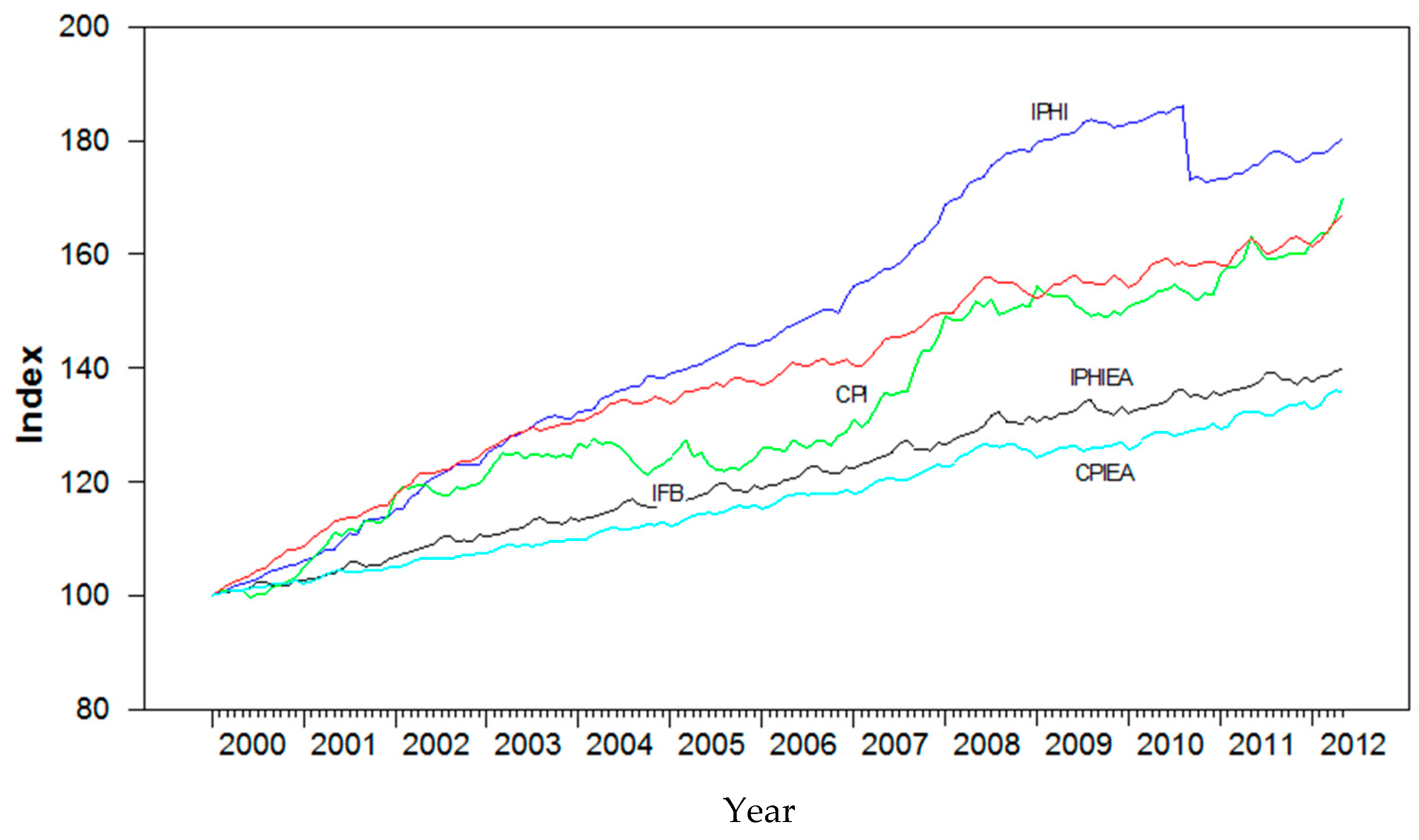
Figure 1. Price indices in levels (base period January 2000). Data vector January 2000 to May 2012 (Great Depression).
Jrfm 14 00517 g001
Figure 2. Unit roots matrix.
Jrfm 14 00517 g002
Figure 3. Price indices in the second difference. Data vector January 2000 to May 2012 (Great Depression).
Jrfm 14 00517 g003
Figure 4. Logarithmic Slovenian food and beverages price index. Data vector January 2000 to May 2012 (Great Depression).
Jrfm 14 00517 g004
Figure 5. Logarithmic Eurozone price index in the hospitality industry. Data vector January 2000 to May 2012 (Great Depression).
Jrfm 14 00517 g005
Figure 6. Logarithmic Slovenian price index in the hospitality industry. Data vector January 2000 to May 2012 (Great Depression).
Jrfm 14 00517 g006
Figure 7. Logarithmic consumer price index in the Eurozone. Data vector January 2000 to May 2012 (Great Depression).
Jrfm 14 00517 g007
Figure 8. Logarithmic Slovenian consumer price index. Data vector January 2000 to May 2012 (Great Depression).
Jrfm 14 00517 g008
Figure 9. Eurozone price index in the hospitality industry I ( 1 ) . Data vector January 2000 to May 2012 (Great Depression).
Jrfm 14 00517 g009
Figure 10. Slovenian food and beverages price index I ( 1 ) . Data vector January 2000 to May 2012 (Great Depression).
Jrfm 14 00517 g010
Figure 11. Slovenian consumer price index I ( 1 ) . Data vector January 2000 to May 2012 (Great Depression).
Jrfm 14 00517 g011
Figure 12. Consumer price index in the Eurozone I ( 1 ) . Data vector January 2000 to May 2012 (Great Depression).
Jrfm 14 00517 g012
Figure 13. Slovenian price index in the hospitality industry I ( 1 ) . Data vector January 2000 to May 2012 (Great Depression).
Jrfm 14 00517 g013
Table 1. Descriptive statistics of nominal price indices (base period January 2000), data vector for 2000–2012.
Descriptive StatisticsCPICPIEAIPHIIPHIEAIFBVAR Model
Mean138.35116.95149.15120.64132.88
N149149149149149
Minimum100.00100.00100.00100.0099.69
Maximum166.83136.10186.07139.80169.87
Skewness−0.0880.211−6.7630.1160.312
Kurtosis2.9673.88771.4604.63234.301
ARCH test0.0520.0210.0010.63011.953 ***234.993 ***
Normality test0.3156.846 **1070.988 ***15.852 ***10.708 ***1082.693 ***
LM test 48.726 ***
Trace or rank test r = 2
Number of lags p = 1
Note: IPHI—Slovenian price index in the hospitality industry, CPI—consumer price index in Slovenia, CPIEA—consumer price index in the Eurozone, IPHIEA—Eurozone price index in the hospitality industry, IFB—Slovenian food and beverages price index. **, ***: significance at 5%, and 1% levels.
Table 2. Misspecification test of real price indices.
Miss–Variables R H P t R P t R F B P t d P E A t 1 d P H E A t 1
Skewness0.350−0.081−0.2090.120−0.140
Kurtosis2.9582.4383.6283.2743.274
ARCH test1.275(0.529)4.591(0.101)0.015(0.992)6.005(0.05)0.696(0.706)
Normality test3.399(0.183)1.860(0.394)4.140(0.126)1.531(0.465)1.597(0.450)
R20.8940.5280.7150.8620.977
Model
Trace or rank test r = 3
ARCH
test
(1): 207.211(0.797)
(2): 462.989(0.326)
Normality test11.570(0.315)
Number of lags p = 2
LM
test
(1): 22.767(0.591)
(2): 30.705(0.199)
Note: R H P t —Slovenian price index in the hospitality industry, R P t —consumer price index in Slovenia, R F B P t —Slovenian food and beverages price index, d P E A t —consumer price index in the Eurozone, d P H E A t —Eurozone price index in the hospitality industry. Significance levels p-value in the brackets, R2—adjusted deterministic coefficient, R —(nominal to) real.
Table 3. A structural representation of the cointegrating space.
Variable β 1 β 2 β 3 α 1 α 2 α 3
R P H t 0.004
(3.508) ***
0.006
(3.284) ***
0−10.114
(−6.407) ***
7.260
(6.645) ***
−3.710
(−5.340) ***
R P t 0−0.004
(−3.333) ***
0−10.930
(−6.834) ***
7.812
(7.058) ***
−3.873
(−5.503) ***
R F B P t 00−0.005
(−4.209) ***
−5.405
(−1.520)
4.493
(1.826) **
−2.356
(−1.506) *
d P E A t 1 11−0.866
(−37.782) ***
1.817
(1.649)
−2.114
(−2.810) ***
0.679
(1.400)
d P H E A t 1 −0.397
(−23.792) ***
010.175
(0.251)
−0.822
(−1.709) *
−0.824
(−2.694) ***
dummy000.001
(3.835) ***
C0.002
(−8.473) ***
−0.003
(−7.035) ***
0
Note. abbreviations already described above, C—constant. Significance levels p-value in the brackets. *, **, ***: significance at 10%, 5%, and 1% level.
Publisher’s Note: MDPI stays neutral with regard to jurisdictional claims in published maps and institutional affiliations.