1. Introduction
The construction industry is an important part of the Polish economy, as it generates from several to a dozen percent of Poland’s GDP (
Rozkrut et al. 2020). For example, in 2018, the construction industry accounted for nearly 10.7% of Poland’s GDP. However, considering the strong linkage of the construction sector with other branches, it can be assumed that the impact of this sector on the generation of Poland’s gross domestic product is much higher. Moreover, the construction sector is the second most employed industry in Poland. At the end of 2019, more than 12% of people were employed in the construction industry and this share is steadily increasing (
Gawor 2019). Also, in terms of value, the construction sector is not losing its importance. In 2018, the value of construction and assembly production exceeded the amount of PLN 200 billion. It is also worth noting that the Polish construction sector is diverse and fragmented, as well as strongly interconnected and dependent on many different areas of the economy. What is characteristic for the Polish construction sector is that in its structure the largest share in terms of quantity is held by small companies, i.e., entities employing up to nine people, which often operate locally and are the pillar of local markets (
Bolkowska 2014). The aforementioned trends are also confirmed by numerous studies and analyses. For example, the construction sector has been considered as one of the most significant sectors in the economies of all countries. Reasons for that are its broad and intense linkages with other sectors that stimulate economic development in the country (
Mallick and Mahalik 2010). Furthermore, the construction sector is an important component of gross domestic product and it plays a crucial role in creating jobs for skilled, semiskilled, and unskilled workers. Moreover, its significant impact on generating Gross Domestic Product (GDP) and the construction sector has important social functions—one of them is affecting the quality of life of the local community. According to studies, employment of 100 people in the construction sector creates at least 200 new jobs and stimulates production in other industries (
Bolkowska 2006). This shows the strong impact of the construction industry on the labor market and the real economy. In the literature, we can find many studies that address the role and importance of the construction sector in the economy, analyzed from a wide variety of perspectives (
Ball 1981;
Bon 1992;
Hosein and Lewis 2005;
Elnamrouty 2012;
Lopes et al. 2011). However, it should be emphasized that the relationship could be strongly dangerous for the real economy while the construction sector makes both direct and indirect contributions to the economic output of the country. It may simply add to the total output and wealth of the economy or it may help in the further production process, resulting in enhanced output (
Mallick and Mahalik 2010). Moreover, the construction sector may contribute to the growth of income and output by increasing the levels of employment. This strong relationship between the construction sector and the country’s economy results in the construction industry being one of the most exposed sectors for the crisis.
If we look at the data, we can notice that after the financial crisis in 2009, the highest number of insolvencies in Europe has taken place in the construction industry in which the number of bankrupt firms has increased dramatically (
Bretz 2013). This has led to a deepening of economic problems in many countries, including a decrease in GDP and an increase in unemployment, as well as a reduction in liquidity in many other entities and industries related to the construction sector because of payment congestion. These negative consequences have affected economies in various countries and have highlighted the essential role of insolvency prediction of companies from the construction industry. In this context, a correct measure of firms’ insolvency risk is very important both for internal monitoring purposes and for investors, stockholders, and actual or potential firm’s competitors (
Succurro 2017;
Balina 2018). Especially after the recent financial crisis, there has been a general need to predict insolvency and financial failure of companies. While the bankruptcy of individual companies in the normal condition is, in fact, a positive mechanism for the elimination of unprofitable entities from the market (
Schumpeter 1942), during market turmoil it may significantly disturb economic equilibrium (
Boratyńska and Grzegorzewska 2018).
Forecasting the risk of insolvency and bankruptcy of construction companies is also a significant challenge for the banking sector, which is one of the main providers of capital necessary for construction projects. Moreover, the above-mentioned dependencies between the construction sector and the real economy also constitute a significant risk for the banks because the insolvency of enterprises from this sector may translate into financial problems of other enterprises cooperating with them and which are co-financed by the banking sector (
Allen et al. 2014). Therefore, the process of creditworthiness assessment through the prism of their solvency and ability to continue operations is an important element in conducting banking activity (
Feschijan 2008). Therefore, banks and institutions cooperating with them strive to develop newer and newer methods and tools, enabling them to detect early the threat of bankruptcy or liquidity risk by construction companies and to limit potential losses connected with granting a credit to an enterprise that will have problems with its timely service (
Embrechts 2004).
Generally, the problem of bankruptcy and insolvency prediction has been the subject of numerous studies and has increased over recent years. In the literature, we can find many investigations that reference this topic. During past decades, researchers from multiple social science disciplines have studied the topic of business failure. Some of them focused on its causes and consequences (
Lukason and Hoffman 2014;
Mellahi and Wilkinson 2004) and other focused on tools that could identify the very first symptoms of forthcoming bankruptcy of the company (
Altman 1968;
Martin 1977;
Shumway 2001;
Balina and Juszczyk 2014;
Ogachi et al. 2020). It is worth stressing that both research fields are complementary, while efficient bankruptcy prediction of companies needs a good knowledge of bankruptcy causes and method of its prediction. Moreover, the results obtained may serve as a basis for further research on the analysis of the financial situation of construction companies in terms of their application in banking practice.
In the literature, we can find plenty of research that refers to a different method of creating an efficient tool for the company’s bankruptcy prediction, which could be adopted by financial institution in assessing creditworthiness of construction companies. These methods could be taken into consideration in two ways. In the first approach, we could focus on generals’ model of predicting bankruptcy. In this field, the pioneer was
Fitzpatrick (
1932), who made efforts to select those indicators that were relevant in forecasting bankruptcy. In the next years, this approach evolved, and authors started to apply newer and more advanced methods. For example, in 1968,
Altman (
1968) used linear discriminant analysis to assess a company’s failure, and in 1977 he and his team (
Altman et al. 1977) used square discriminant analysis to construct a bankruptcy prediction model.
Martin (
1977) presented studies taking advantage of logit models to estimate the probability of firm bankruptcy. The next adapted method used for predicting bankruptcy risk was neural network (
Salchenberger et al. 1992;
Yang et al. 1999;
Charalambous et al. 2000), non-linear discriminatory analysis (
Muhamad Sori et al. 2006), analysis based on the theory of entropy (
Merton 1974), support vector model (
Chen et al. 2011), and hybrid methods—essentially combinations of various methods. This shows that the major problem of constructing an effective bankruptcy prediction model is choosing a method of estimating the model.
In the literature, we can find that model analysis based on the applied method indicates that methods do not have a significant influence on effective bankruptcy prediction. As stressed by Balina and Juszczyk (
Balina and Juszczyk 2014), the results of various models oscillate between 80 and 98%, which is recognized as a satisfying level. Considering that the main issue of this research was to develop an insolvency prediction model that can be easily used in practice to analyze and signal the risk of failure of a firm, also the research must identify key financial and organizational factors that would allow for early identification of the symptoms of the deteriorating financial situation of companies from the construction sector.
Therefore, the literature contains many examples of solutions for the early identification of the insolvency risk of construction companies (
Marcinkevičius and Kanapickienė 2014;
Arditi et al. 2000;
Heo and Yang 2014). However, these models ignore the influence of external factors on the risk of insolvency. Therefore, this paper aims to develop a model for predicting the risk of insolvency of construction companies using financial data reflecting the financial situation of the company, its position in the industry, and the impact of selected external factors unique for construction companies. Such an approach to research will, on the one hand, fill the hitherto existing research gap concerning the incorporation of external factors in models for forecasting insolvency or bankruptcy of construction companies and, on the other hand, provide a comprehensive tool for assessing the risk of insolvency of such companies. What is more, the paper considers the use of industry variables and the market situation in the construction industry as an element to better predict the insolvency risk of construction companies. To date, a limited number of such attempts has been made in the literature. In addition, the article, through the use of a broad set of variables and various methods, points to important areas of construction companies’ operations that may indicate their risk of insolvency. Therefore, stakeholders are provided with a practical tool to assess the risk of insolvency of construction companies, which takes into account not only the company’s situation but also external conditions
The article consists of four parts. In the first one, the rationale for the research undertaken and a review of the literature on forecasting the insolvency of construction companies is presented. Afterwards, characteristics of the research sample and applied estimation methods for construction companies’ insolvency risk assessment (discriminant analysis, logit regression and regression trees) are presented. Then, the results of the research on the selection of variables for the study and the results of estimation of models of construction companies’ insolvency are presented. Finally, the effectiveness of the estimated models is assessed and the results and limitations of the research are summarized.
2. Materials and Methods
The analysis was based on a sample of data from 80 companies operating in the construction industry in the years 2014–2018 in Poland as limited liability companies, which represents 4.76% of all construction companies operating in Poland in 2018 (
Płatek 2020). The date was composed of two groups of companies. The study considered 40 insolvent companies from the construction industry, which published annual financial reports for at least three full accounting periods before they announced insolvency in 2018. These entities accounted for 28.57% of all enterprises that declared insolvency in 2018 in Poland (
Padzik 2019). To the opposing side, 40 companies were chosen that were operating in 2018 since 2014 and had similar asset values to the bankrupt companies, with differences no greater than 25% of the average of the total assets of analysis companies.
The relevant indicators were selected for the financial statement analysis and assessing the financial condition of analyzed companies. The financial statement analysis allows for a company-wide point of view, not the owners’ expectations. The financial statement analysis consists of indicators in the literature (
Karminsky and Burekhin 2019;
Alaminos et al. 2016). First, a basic financial analysis of the collected financial statements was made. During the research, financial indicators were analyzed, which included asset and liability structure, liquidity ratios, profitability ratios, operational efficiency indicators, debt ratios, and selected values of assets and liabilities. Additionally, the list of analyzed indicators was supplemented with the factors presenting the value difference of a quick ratio, current ratio, cash ratio, return on assets, return on equity, return on sales, return on current assets, and cost-to-income ratio and the average of the indicator for the construction industry, determined by the Central Statistical Office of Poland. To fulfill the scope of the analysis, the dynamics of the following categories were used: sales revenue, total assets, current assets, fixed assets, total equity, foreign capital, current liabilities, operating result, and net result. In the study industry-related indicators were applied to demonstrate the influence of the main factors having an impact on this sector. It should be noted that solvent companies were assigned a value of 1 (one), and bankrupted companies were assigned a value of 0 (zero). In
Table 1 the descriptive statistics of the analyzed companies are shown.
When choosing estimation methods of models to evaluate the risk of insolvency of construction companies, the sample of 80 observations was taken into account, including 40 solvent companies and 40 insolvent companies. The sample, due to the specificity of the subject matter and geographical range, met the requirements of representativeness, however, due to its small size it could translate into certain limitations resulting from the adopted research methodology. Considering the study by
Roscoe (
1975) who found that a sample between 30 and 500 observations is sufficient for building multivariate models and also other attempts to apply multivariate methods with a small sample (
Marini 2010;
Paul et al. 2008;
Rainey and McCaskey 2015;
Motrenko et al. 2014;
Ślaska-Grzywna 2010;
Morgan et al. 2001), it can be concluded that the sample adopted for the study is sufficient. Furthermore,
Sharma and Paliwal (
2015) emphasize that there is no predetermined rule for deciding the sample size and it depends on the type of data and the hypothesis being designed.
Having mainly the goal of the study and sample size limitations, authors decided to use three different approaches to the model’s estimation. In this study we use a linear discriminant function, logistic regression, and classification trees. The preference for the model’s estimation methods was dictated by the idea that the result of model estimation should be easily applied, which is in accordance with one of the fundamental precepts in applying models for assessing a company’s condition.
The discriminant analysis depends on estimating a linear discriminant function, allowing for the differentiation of studied multi-dimensional collections through designating linear combined qualities, which differentiate two or more class objectives (
Gatnar 1999). Linear Discriminant Function appears as such (
Lachenbruch and Goldstein 1979).
where:
—discriminant coefficients,
—variable diagnostic value.
The logit model is classified among the classical models of binary classification, that is, where the explanatory variable is a qualitative variable taking two values. In the logit model, the linear combination of features supplemented with a free expression is transformed by a logistic function. What is more, the logistic regression model assumes that the probability of a dichotomous outcome is related to a set of potential predictor variables in the form (
Witkowska 2006):
where
p is the probability of the outcome of interest,
is the intercept term, and
(
i = 1, ...,
n) represents the b coefficient associated with the corresponding explanatory variable
(
i = 1, ...,
n).
The classification regression trees are used to determine the membership of cases or objects in classes of a qualitative dependent variable based on measures of one or more explanatory variables (predictors). Moreover, classification regression trees are used to construct predictive classifiers
Y ∈ {1, 2, …, g} based on a p-dimensional vector of attributes (arbitrary attributes: nominal, nominal on ordinal scale, continuous) or to construct regression function estimators as (
Loh 2011):
where
ε is a random error such that
Eε = 0.
To confirm the accuracy of the model, the efficiency of the model was checked with the accuracy matrix proposed by Altman (
Altman 1968). Having in mind the main goal of this paper, we estimated four different models to predict insolvency of construction companies.
3. Results and Discussion
To determine the key indicators revealing the insolvency risk of enterprises from the construction industry, in the first stage of the research, the predictive power of each variable was determined using the Information Value Index (IV) proposed by
Hand and Henley (
1997).
Table 2 presents the results on the estimated values of the Information Value Index for the analyzed set of variables.
The results showed that all of the analyzed variables were characterized by the value of the IV coefficient exceeding the minimum significance level of 0.02. Additionally, it should be emphasized that this level was higher than 0.1, which, according to the literature, indicates the appearance of at least moderate strength of belonging to a given group. This indicates the usefulness of all the variables considered in assessing the insolvency risk of construction companies. Also, at this stage of the research, explanatory variables that were weakly correlated with each other were sought. During the research, it was determined that the critical value of the correlation coefficient for the considered set of variables was: r* = 0.220. This selection of variables avoided the problem of collinearity in the model, which was confirmed by calculating the VIF (Variance Inflation Factor) statistic. Having in mind this assumption, key economic and financial indicators were chosen. This set of factors was crucial in the insolvency prediction of construction companies in Poland. The conducted analysis established that 19 out of the original explanatory variables were statistically significant: X2; X5; X6; X8; X9; X10; X12; X17; X19; X20; X21; X27; X28; X30; X31; X35; X36; X37; and X41.
Of the 19 indicators, three, X35; X36; and X37, characterized the pace of changes in such economic categories: fixed assets, equity, and foreign capital, respectively. The next four indicators: X27; X28; X30; and X31 determined the deviations between the ratios—profitability of current assets, profitability of fixed assets, liquidity between their average values in the examined industry, and their values obtained by the examined enterprise, respectively. The X41 index represents the level of sales dynamics of the surveyed company adjusted by the change in the average price per square meter of usable floor area of buildings in Poland. Other indicators characterized the share of current assets in the structure of total assets, turnover of receivables in times, turnover of liabilities in times, the relation of total assets to equity, and the ratio of sales revenues and total assets of the enterprise.
The first model to be developed was discriminant analysis (ZAD) estimated by using the classical least squares method using backward stepwise regression, with the help of Student’s t-test, which enabled the construction of an optimal discriminant function. The construction of the discriminant function involved selecting the variables in the model such that the variance-covariance matrix was well-conditioned, and the parameters of the discriminant function could be estimated. The models were estimated using backward stepwise analysis, with the removal of variables from the model based on the value of the
p-value statistic (
Sharma and Paliwal 2015). Thanks to this approach, only those variables remained in the model whose discriminatory ability corresponds to the imposed criterion. Based on the assumptions and the collected data, the discriminant function was estimated and the results are shown in
Table 3.
For the estimated model, the Wilks lambda statistic is 0.50432 and the corresponding F-test statistic is F(5.74) = 14.547 and
p-value < 0.000. Also, the selection of variables avoided the problem of collinearity in the model, which was confirmed by calculating the Variance Inflation Factor (VIF) statistic (
Lachenbruch and Goldstein 1979;
Hand and Henley 1997). This indicates an acceptable level of quality of the estimated model. In accordance with the methodology, it was assumed that the cut-off point of the estimated discriminant function is exactly halfway between the expected values of the distributions of each class in the sample. Thus, by determining average values of the discriminant variable in both classes, the threshold of the discriminant function was considered to be their average value (
Balina and Juszczyk 2014). For the model, ZAD was considered a cut-off point at a level of 0.22.
When analyzing the obtained ZAD model in terms of content, it should be emphasized that three of the four indicators that eventually found themselves in the model have a negative regression coefficient. These are the following indicators: X28; X30; and X36. The first of them (X28) determines the number of deviations of the value of the current assets’ profitability ratio for the industry from the value obtained by the audited enterprise. This indicates the positive consequences of increasing the profitability ratio of the company’s current assets above the average value for the industry, because in this case, the value of this variable has a positive effect on the aggregate value of the constructed discriminatory function. The above can also be applied to the X30 ratio, which reflects the difference between the average quick liquidity ratio for the industry and the value of this ratio for the enterprise. A negative indicator value combined with a negative sign of the parameter gives a positive final value. Construction companies are recognized as justified, because they are in an industry that is characterized by a high degree of competition and connections between entities. Maintaining a sufficiently high level of quick liquidity by the company and the profitability of current assets above the industry average allows for free settlements of the company’s liabilities and enforces efficiency of operations, thus reducing the risk of bankruptcy.
The third indicator with a negative factor (X36) expresses the rate of change inequity in the base year to the previous year, and its positive value adversely affects the value of the discriminatory function. Increasing equity capital reduces the final value resulting from the model, which translates into an increased risk of bankruptcy. It is worth noting that regardless of the direction of changes in equity, it reduces the value of the ZAD function. However, the increase in equity with each year is more undesirable than its decrease. This suggests the need for development based on foreign, relatively cheaper sources of enterprise financing.
The positive coefficient of the discriminant function with variable X2 significantly indicates the share of current assets in total assets of construction companies. This indicates the importance of construction companies maintaining an adequate level of current assets necessary for their day-to-day operations. The X20 indicator, which has a positive parameter in the ZAD model, expresses the relation of sales revenues to total assets. This means that the higher the value of the asset utilization ratio, the lower the risk of bankruptcy of the audited entity, assuming ceteris paribus. This relationship is desirable from an economic point of view, as the higher value of this indicator indicates a better use of the entity’s assets to generate sales revenues.
The second model was estimated using a logit regression function, where ZRL is the power exponent in the model, allowing for the assessment of the insolvency risk of companies in the construction industry. The model was estimated using backward stepwise analysis, with the removal of variables from the model based on the value of the p-value statistic. Thanks to this approach, similarly, like in the ZAD model, only those variables remained in the model, whose discriminatory ability corresponds to the imposed criterion. What is important is thatall variables that were found in the estimated model were statistically significant at the given level of significance, and also variables were characterized by the lack of collinearity, which was confirmed by the values of VIF statistic. The results of estimation are shown in
Table 4.
For the model, ZLR was considered a cut-off point at a level of 0.5, which was in line with the literature (
Motrenko et al. 2014).
There were six variables in the logit function determining the level of insolvency risk of companies in the construction sector. The first variable determined the structure of the company’s assets, where X2 determined the share of current assets in total assets. The second variable (X8) determined the relation of sales revenues to current liabilities. This indicates the importance of the formation of this structure in the functioning of construction companies in Poland. In addition, in this industry, the increase in the share of current assets in the assets of enterprises was desirable, while the increase in the share of fixed assets in the total assets of construction companies contributed to the increase in the risk of insolvency and, consequently, their bankruptcy. This could be due to the specificity of this industry, where the companies in this industry earn revenue from the sale of fixed assets, and the maintenance of current assets is associated with costs resulting from the failure to complete investments.
Another variable determined the relationship of total assets of the company to its equity (X17). It should be noted that this variable was characterized by a negative regression coefficient, and this indicated the need to maintain a relatively high level of equity in relation to the assets of the company, which could translate into greater financial security of the company, and thus reduce the risk of its insolvency and allow uninterrupted implementation of investments. Variable X20 determined the profitability of total assets of the company, which indicated that companies in the analyzed industry, to avoid the risk of insolvency, should strive to increase revenue per unit of assets used to generate them, so as to increase the profitability of sales of implemented projects. The next variable X28 determined the profitability of current assets of the company against the background of the industry. The estimated model indicates that construction companies should maintain the level of this indicator at a level close to the industry average or above the industry average value, because the maintenance of current assets in construction companies involves costs and immobilization of cash; therefore, construction companies should strive to increase the profitability of these assets to reduce the risk of insolvency. The last variable determines the sales dynamics of the company adjusted by the index of price changes of construction and assembly production in the economy. The estimated model indicated that in the case of construction companies, it is important that sales revenues grow faster than the average price level of construction and assembly production in the whole economy, which should translate into the company’s ability to generate more added value from the investments sold.
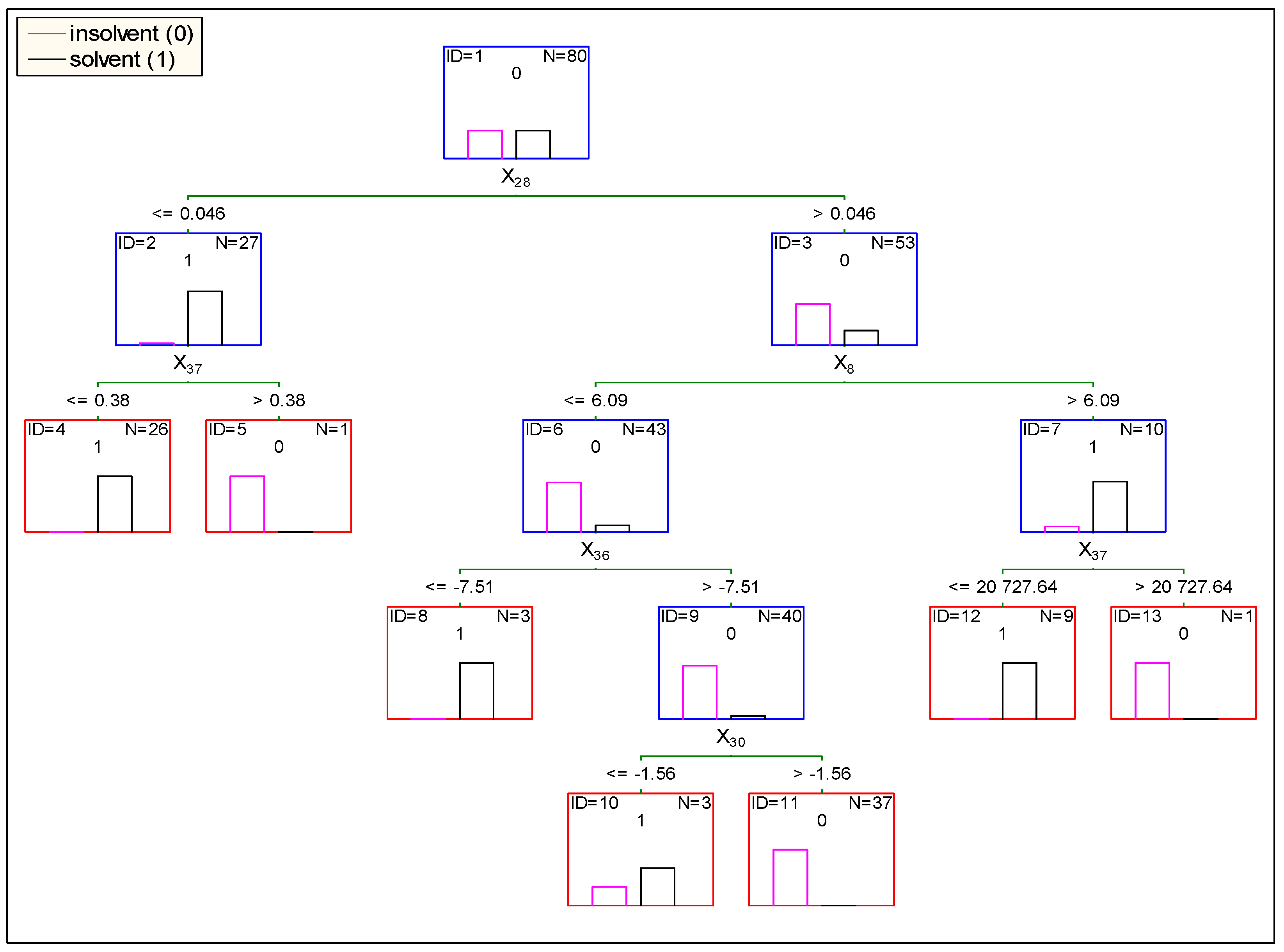
In the next step, the model of insolvency risk assessment of construction companies was estimated using classification trees (ZRT). To estimate the classification trees, we used CHAID (Chi-square Automatic Interaction Detection), which was firstly introduced by
Kass (
1980). CHAID is an analysis based on a criterion variable with two or more categories. This allows researchers to determine the classification with respect to that variable and in accordance with the combination of a range of independent variables. In consideration of the approach adopted, a p-value of 0.05 and a minimum node-forming case count of 10 were used as parameters to control the growth of the classification tree. With this in mind, a classification tree was estimated in which five variables were included i.e., X
8—determining the current liabilities revenue ratio, X
28—determining the profitability of current assets of the company in comparison with the industry, X
30—indicating the level of immediate liquidity in comparison with the industry, X
36 determining the dynamics of equity, and X
37 referring to the dynamics of foreign capital. In the case of the estimated regression tree, these variables were the basis for determining the category of division of enterprises into groups and making the final classification.
Figure 1 presents a diagram of the developed regression tree (ZRT) along with the values based on which the division into individual branches was made.
As can be seen from the presented scheme, finally in the tree seven paths were distinguished, based on which it was possible to classify construction companies in terms of insolvency risk.
Table 5 presents a summary of the occurrence of variables in each model. The summary indicates that in all estimated models the variable X
28 determining the level of profitability of current assets of the construction company in comparison with the industry was significant, which may indicate that this element is crucial for maintaining liquidity and financial security by construction companies. Additionally, it is worth noting that variables such as X
2, X
8, X
20, X
30, and X
36 were present in two of the three models developed. Therefore, it can be assumed that these variables also had a significant impact on the insolvency risk of the companies in the industry under study. The remaining variables, i.e., X
17, X
37, and X
41 occurred in only one of the three developed models, nevertheless their appearance in the developed solutions could indicate their importance in the process of liquidity management and financial security of these entities. It is also worth noting that the variables that were included in the developed models concerned a diverse area, determining the financial situation of the company, but also took into account the relationship between the company and its environment, which was a significant advantage of the estimated models over previous solutions.
In the next step, the obtained results were subjected to statistical and fundamental analysis to determine the quality of the developed model and its economic requirements. At this stage, it was assumed that the model should have efficiency exceeding 80%. To confirm the accuracy of the model, the efficiency of the model was calculated with the accuracy matrix proposed by
Altman (
1968). In
Table 6 we presented an accuracy of constructed model.
The first performance degree that shows the correctness of recognition of the insolvent entities (SP1) for the model ZAD was 95%, which means that 38 out of 40 companies were rated as insolvent and were rated correctly. For model ZLR, the efficiency of recognition of insolvent companies was at the same level as the ZAD model—95%, but the ZRT model was characterized by 100% efficiency in recognition of the insolvent companies. This indicates a high level of effectiveness of the developed models, with the model based on regression trees being the most efficient. However, if we look at the level of accuracy of identification of solvent companies, we observe major discrepancies. The second degree performance (SP2) of the ZAD model was 70%; in case of the ZLR model, it was 95%; and in the ZRT model, the efficiency of proper classification of solvent companies reached 100%. On this basis, it should be concluded that the ZAD model insufficiently recognizes solvent companies, however, taking into account risk mitigation, the lower level of effectiveness of the model in this area is not as significant as in the case of the first-degree accuracy. If we look at overall performance (SP0), an accurate rating of all analyzed companies by the ZAD model was 82.5%. In the case of the ZLR model, the level of model efficiency SP0 reached 95% and in ZRT model this level reached 100%. This is a moderately satisfactory result and allows the model’s effective application in business practice to establish bankruptcy risk for companies in the construction sector. To confirm the effectiveness of the estimated model, the testing sample was used. This sample was composed of 80 companies from the industry sector, 40 bankrupt and 40 non-bankrupt companies. Effectiveness verification of estimated models on the test group indicated that overall bankruptcy forecast performance in the case of construction companies for ZAD model was 90.0%, for ZLR model was 96.25%, and for ZRT model was 97.50%. The components of this assessment are the high accuracy of identifying solvent companies in all models that surpassed a level of 92.50% and higher performance in identifying bankrupt companies at a minimum level of 87.50%. What is more interesting in the case of ZAD and ZLR models is that the level of general model efficiency was higher than in the learning sample, and in the ZRT model we observe a decrease in its efficiency, but even in this situation the partial and overall efficiency of ZRT model was higher than in the remaining models.
4. Conclusions
The article deals with an important issue of forecasting the risk of insolvency of companies from the construction industry, which is one of the most important pillars of the economy in many countries around the world. Moreover, the paper considers the use of industry variables and the market situation in the construction industry as an element to better predict the insolvency risk of construction companies. To date, no such attempt has been made in the literature. In addition, the article, through the use of a broad set of variables and various methods, points to important areas of construction companies’ operations that may indicate their risk of insolvency. Therefore, the results can provide a valuable source of information for both the managers of construction companies and external stakeholders, including owners and cooperators.
The results of the empirical study provided several interesting findings. First, the choice of the model estimation method for assessing the insolvency of companies in the construction sector affected the range and number of variables included in the estimated model and the efficiency of a given model. However, in the case of three estimated models, which in total included nine different variables, all of them included variable X28, which means that in the case of the construction industry, an important element indicating the solvency of companies in this industry is the level of profitability of current assets of a given company exceeding the average level of profitability of current assets in the construction industry. This may result from the fact that in most cases the companies from the construction industry employ current assets required to provide construction works in their day-to-day operations, and this activity is their basic revenue source. Therefore, maintaining the current assets’ profitability above the industry average may enable construction companies to maintain their solvency. What more, variables X2, X8, X20, X30, and X36 were included in two models. These results indicate that to maintain financial security and solvency, construction companies should maintain quick liquidity above the industry average, which is directly related to their ability to pay their current liabilities. Moreover, the companies should seek to increase the revenue ability of total assets and revenue ability of current liabilities. This is due to the fact that construction companies use their assets for day-to-day operations and, according to the theory of finance, these assets should generate the highest possible revenues. In addition, it is important that construction companies also tend to maintain a higher level of income from current liabilities, because they often use short-term loans or merchant credits in their operations, so, in order to maintain solvency, they should use these liabilities as efficiently as possible. The models also indicated the importance of construction companies maintaining positive dynamics of equity, which contributes to increased financial security of these entities and their solvency. This shows that despite the use of different methods, the key determinants of financial security of construction companies, indicated by the estimated model, converge. Therefore, it can be concluded that the choice of model estimation methods for assessing the insolvency risk of construction companies affects the efficiency of the model on the one hand. On the other hand, the choice of method does not significantly affect the range of factors enabling the identification of liquidity symptoms of these companies.
Based on the study, it was also concluded that constructed models for forecasting the threat of insolvency of enterprises from the construction sector pointed out nine variables that were, in general, key to assessing the risk of insolvency of enterprises in this industry, which is in line with other similar research conducted by
Marcinkevičius and Kanapickienė (
2014);
Mallick and Mahalik (
2010); or
Chen et al. (
2016). These indicators were related to the profitability, revenues, liquidity, asset’s structure, and dynamics of own and foreign capitals, but what is most important is that our research has shown that when we are assessing the insolvency risk of construction companies, factors that refer to the industry and market situation should be taken in to account. This indicates the importance of indicators describing the external conditions of construction sector companies in assessing their insolvency.. Thus, enterprises in this industry should carefully monitor the state of the entire industry and changes occurring in it so that they can react early enough and guard against difficulties and even bankruptcy.
The study involved a limited number of companies from the construction sector; therefore, its scope is limited and provides possibilities for further work in the field when searching for key factors that determine the level of insolvency risk of construction companies, using a wider range of data and diversified multidimensional methods. Also, it should be remembered that these conclusions were drawn based on a research sample of 160 companies, and therefore they should not be attributed as universal characteristics but treated as a basis for deeper analysis in the future in the context of using sectoral variables to predict the insolvency of firms in different sectors of the economy.


