Abstract
This paper examines the connectedness between Bitcoin and commodity volatilities, including oil, wheat, and corn, during the period Oct. 2013–Jun. 2018, using time- and frequency-domain frameworks. The time-domain framework’s results show that the connectedness is 23.49%, indicating a low level of connection between Bitcoin and the commodity volatilities. Bitcoin contributes only 2.55% to the connectedness, while the wheat volatility index accounts for 12.51% of the total connectedness. The frequency connectedness shows that Bitcoin’s contribution to the total connectedness increases from high-frequency to low-frequency bands, and the total connectedness reaches up to 22.47%. It also indicates that Bitcoin is the spillover transmitter to the wheat volatility, while being the spillover receiver from the oil and corn volatilities. The findings suggest that Bitcoin could be a hedger for commodity volatilities.
1. Introduction
Bitcoin is known as a decentralised digital currency that is used in online payment systems and traded in major developed and emerging economies (e.g., USA, China). Thanks to its innovative open-source protocol, Bitcoin is a virtual currency that is not subject to any authority or control such as a national or supranational central bank or financial authority (Böhme et al. 2015; Weber 2016). Given its design protocol, the Bitcoin supply is limited to only 21 million. Bitcoin has risen to prominence since 2008, when the global financial meltdown dented the public’s trust in the global financial system. Its value rose spectacularly from USD 0.008 on 22 May 2010 to nearly USD 20,000 on 17 December 2017. As a result, Bitcoin is the first digital currency that has markedly gained traction to become a major economic instrument (Carrick 2016; Bouri et al. 2017b).
Bitcoin has increasingly received academic attention. A myriad of studies examined Bitcoin from various perspectives, for example, the determinants of Bitcoin prices or returns (Yelowitz and Wilson 2015; Ciaian et al. 2016) and their volatilities (Charles and Darné 2019; Troster et al. 2019). Whereas scores of papers examine the efficiency of the Bitcoin market (Urquhart 2016; Bariviera 2017; Nadarajah and Chu 2017), few studies explore transaction costs (Kim 2017) and informed trading (Feng et al. 2018).
Although several studies argue that Bitcoin contains substantial speculative components (Corbet et al. 2018; Fry 2018; Fry and Cheah 2016), other studies show that Bitcoin has the potential to become an investment instrument. The recent literature further underlines the importance of Bitcoin as a risk diversifier or a hedge against various financial assets, since Bitcoin returns are not associated with those assets. According to Bouri et al. (2017c), Bitcoin is found to be an effective diversifier against general commodities, equities, bonds, and the US dollar.
In this regard, Bitcoin has considerable financial properties as a risk diversifier or a hedge against commodity uncertainty, especially agricultural commodities. To our knowledge, the relation between Bitcoin and commodity uncertainty is unexplored. Commodity prices have experienced dramatic booms and bust cycles (Mensi et al. 2017). The prices of commodities, such as agricultural products and oil, tend to be highly volatile. Oil price volatility could be due to various reasons, including geopolitical tensions and agricultural commodity prices, which also vary dramatically, particularly along with energy price fluctuations. The more volatile the commodity prices, the more difficult and costlier the risk management of commodity prices for both producers and consumers (Wu et al. 2011). The damages spawned from commodity price volatility are socially and economically tremendous. Due to price spikes and the scarcity of agricultural commodities, severe economic hardship, and possibly socio-political tensions, are sometimes unavoidable (Mensi et al. 2017). From another approach, Bianchi (forthcoming) shows that there is a mild correlation between the returns on commodities and cryptocurrencies, but this linkage does not exhibit in volatility spillover effects.
For the previous reasons, discovering the sign and size of the association between Bitcoin and commodity uncertainty is profoundly important, from the perspective of investments and portfolio risk management. The findings are essential for market participants to make informed decisions for their investments and provide implications for portfolio management. Therefore, this paper aims to investigate the connectedness between Bitcoin and the volatilities of the most popularly traded commodities, which are corn, oil, and wheat.
Our current research contributes to the literature in three ways. First, it is the first research that attempts to investigate the connection between the financial innovation Bitcoin and commodity uncertainty, using the newly-developed time-domain connectedness suggested by Diebold and Yilmaz (2012), based on the vector autoregression (VAR) model and the frequency-domain connectedness presented by Baruník and Křehlík (2018). These methods allow us to figure out the contribution of Bitcoin to different commodity volatilities and, at the same time, to find out whether Bitcoin is a volatility transmitter or a receiver at different frequencies. Second, our study also analyses the time-varying connectedness between commodity volatilities and Bitcoin at different frequencies, to show a panorama of their linkages from 1 day, 4 days, 10 days, and to infinity.
Third, this study uses the forward-looking commodity uncertainty indices, including corn, oil, and wheat volatility indices, rather than the volatility calculated from historical prices or the model-based volatility (e.g., GARCH-based volatility model). Market participants are more concerned with the future volatilities of commodities where there is a need for risk management strategies. The oil, wheat, and corn volatility indices measure the market expectation of volatility generated from the option prices of these commodities (CBOE 2018).
2. Literature Review
Academic interests in Bitcoin have increasingly grown in recent years. A number of studies focus on testing the “efficient market hypothesis” of the Bitcoin markets. Urquhart (2016) and Nadarajah and Chu (2017) reveal that the Bitcoin market is inefficient. Bariviera (2017) also finds that the Bitcoin market is not efficient, despite it becoming more informationally efficient since 2014. This conjecture is supported by recent studies in the literature (Vidal-Tomás and Ibañez 2018; Tiwari et al. 2018; Kyriazis 2019). In summary, the efficient market hypothesis seems invalid for the Bitcoin market.
Another line of literature studies the volatility of Bitcoin prices or returns. Recent research works in this literature strand investigate various aspects of the volatility and provide enriched findings (Chaim and Laurini 2018; Klein et al. 2018; Koutmos 2018; Ardia et al. 2019; Charles and Darné 2019; Kyriazis et al. 2019). By applying the VAR model, Koutmos (2018) indicates that Bitcoin plays a role as the major contributor to returns and volatility spillovers among 18 cryptocurrencies, indicating a high degree of contagion risk. Kyriazis et al. (2019) indicate that the volatility of most cryptocurrencies during the bearish period is complementary with the volatility of Bitcoin. Katsiampa (2017) suggests using autoregressive-component GARCH (AR-CGARCH) to model the optimal conditional heteroskedasticity of Bitcoin prices. With the purpose of performing a replication and checking the robustness of Katsiampa (2017)’s study, Charles and Darné (2019) show partially different results, due to the differences in calculating Bitcoin returns. However, the authors argue that the application of six GARCH-typed models seems to not be suitable for modeling the Bitcoin returns.
A major strand of the literature investigates the determinants of Bitcoin prices or returns by employing primarily daily prices. Ciaian et al. (2016) show that the price of Bitcoin is mainly conditioned on the demand side (e.g., daily frequency of Bitcoin transactions), given that the supply side is pre-determined. Bitcoin price seems not to be affected by the same factors as those of conventional assets, such as commodities, equities, and bonds. To be specific, the price of Bitcoin is interestingly stimulated by the number of internet searches (Kristoufek 2013; Yelowitz and Wilson 2015). Moreover, Ciaian et al. (2016) find that Bitcoin prices are not determined by macro-economic developments such as oil prices and exchange rates. Polasik et al. (2015) provide evidence that the returns of Bitcoin investment are driven largely by Bitcoin popularity, sentiments in media reports, and transaction numbers. It is noteworthy that Bitcoin prices differ significantly across exchanges due to different exchange settings, especially the failure of the exchange to require customers to expose their identities (Pieters and Vivanco 2017).
Bitcoin prices appear to be driven by speculation (Baek and Elbeck 2015; Ciaian et al. 2016; Kyriazis et al. 2019), echoing the previous finding by Cheah and Fry (2015), that Bitcoin constitutes a substantial speculative component. Fry (2018) reiterates that Bitcoin is speculative in nature and provides evidence of Bitcoin price bubbles. The finding is further supported by Corbet et al. (2018), who reveal that Bitcoin prices exhibit the stages of bubbles, and Bitcoin has been in the bubble phase since the moment its price exceeded USD 1000. The literature seems to underline that Bitcoin is not driven by the same economic or financial fundamentals of conventional financial assets.
Although Bitcoin seems to be used as a speculative investment, it has considerable potential as a risk diversifier or a hedger. Baur et al. (2018) find that no association is found between Bitcoin and conventional assets such as commodities and securities, in either normal or financial turmoil periods. By examining general cryptocurrencies, Baumöhl (2019) provides evidence of a negative correlation in short and long terms between forex and cryptocurrencies; thus, it is worth diversifying between the two assets. Dyhrberg (2016a) states that Bitcoin should be, characteristically, defined as a hybrid investment instrument that is classified between commodities and currencies, because of its decentralised nature and restricted market dimension. Thereby, it can be a good instrument for market sentiment analysis, portfolio management, and risk analysis (Catania et al. 2019). Specifically, Dyhrberg (2016b) underscores the hedging capability of Bitcoin against the fluctuations in the UK stock market and the US dollar. Beneki et al. (2019) find that Bitcoin can be a hedger for Ethereum. Kyriazis (2020) shows that Bitcoin is an effective hedge against oil and stock market indices. Similarly, Bouri et al. (2017a) find that Bitcoin is a good choice for diversification against securities, gold, commodities, oil, and the US dollar. The authors also indicate that, before the December 2013 crash, Bitcoin is a diversifier against the US equity portfolios and even presents a safe-haven property, although investors ought to be wary of its lack of liquidity. Bouri et al. (2018) lend further support to the previous finding that Bitcoin can play the role of a shelter against global financial meltdown from the medium-term viewpoint. Bouri et al. (2017c) provide empirical evidence that Bitcoin can serve as a hedge against risks in the short-term investment horizon, given a bull market condition. Demir et al. (2018) further signify the hedging role of Bitcoin in extreme times of uncertainty.
3. Methodology
In this study, we apply the dynamic variance decompositions vector autoregression (VAR) model from Diebold and Yilmaz (2012), and the frequency-domain connectedness presented by Baruník and Křehlík (2018), to examine interdependence or connectedness between variables. The benefit of using these models is that the forecast error variance decompositions are invariant to the ordering of the variables in the VAR, and it also allows for correlated shocks rather than orthogonalizing shocks. In addition, it enables us to figure out the connectedness over time, since any time-varying dependence is of great interest.
Let the following model be the structural VAR (p) at t = 1, …, T: where εt denotes white-noise and Φ(L) is the pth order lag-polynomial matrix computed as .
Diebold and Yilmaz (2012) define the connectedness measure as:
where
and:
is the generalized forecast error variance decomposition (FEVD); σmm = (∑)mm; and ψh stands for an nxn matrix of coefficients with lag h, Tr {·} is the trace operator. SH is the connectedness of the whole data sample, while the directional spillover from one variable to another can be measured in the same way.
Baruník and Křehlík (2018) define the frequency connectedness on band d, where:
and
The band d’s within frequency connectedness is as follows:
where the generalized FEVD on different frequency bands d is specified as:
and
is the weighting function, while the frequency response function is defined as:
In addition, our aim is to examine if Bitcoin and the commodity volatilities are strongly correlated. If they are, there will be no case that Bitcoin can be a hedger for the commodities. As a robustness test for our results, we choose the time-varying mixed copula of Joe–Clayton, because it can simultaneously reveal the existence of the left and right tail dependence over the examined period. The left and right tail dependences represent the likelihood of crashing and booming together of variables, respectively. If the variables have no left tail dependence, it will be beneficial to include them into a portfolio, since if one crashes, the other will not.
Following Patton (2004), we use the symmetrized Joe–Clayton copula (SJC copula), for checking the robustness of our findings. The function of the SJC copula is presented as follows:
in which CJC represents the SJC copula function; u and v are the innovation obtained from AR process of two variables (X, Y). τU ϵ (0,1] is the upper tail and τL ϵ (0,1] is the lower tail. The time-varying tail dependencies are modelled as follows:
where
The results will be presented in Section 4.2 and Section 4.3.
4. Data Analysis
4.1. Data
We proxy commodity uncertainty using three implied volatility indices from October 2013 to June 2018, including the corn index (CVI), the crude oil index (OVX), and the wheat index (WVI), which first started in Oct 2013. The daily data for these indices are extracted from the Bloomberg database. We collect the Bitcoin Price Index (BPI) from Coindesk (www.coindesk.com/price/bitcoin). Specifically, the BPI is computed as the average of Bitcoin prices across different Bitcoin exchanges. Therefore, it can neutralise the differences in Bitcoin prices from different cryptocurrency exchanges and is a good proxy for Bitcoin worldwide.
We use log data for our analyses with the total observations for each series of 1285. Time-series plots for the three commodity indices and Bitcoin are illustrated in Figure 1. In Figure 1, part (a) shows that OVX is quite volatile during 2014–2016, due to the booming U.S. shale oil production and the shifting of OPEC policies. The other two indices are fairly stable, fluctuating within a certain range. Part (b) presents an interesting story when it comes to Bitcoin prices. The Bitcoin price remained low until the end of 2016, when there was a growing interest in cryptocurrencies. This led to an increase of more than 400% for Bitcoin prices in 2017.
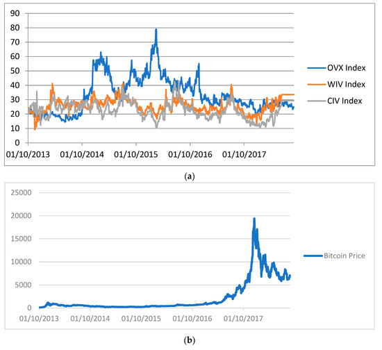
Figure 1.
The developments in the crude oil index (OVX), the wheat index (WIV), the corn index (CIV), and the Bitcoin Price Index (BPI), from October 2013 to June 2018. Part (a) shows the movement of OVX, WIV, and CIV indices during the period from October 2013 to June 2018. Part (b) illustrates the developments of Bitcoin price during the period from October 2013 to June 2018.
Table 1 summarises the descriptive statistics. All data series are stationary since they all pass Jarque–Bera and augmented Dickey–Fuller (ADF) tests. As usual, the returns from all indices are quite small, while that of Bitcoin looks promising since its return averaging 0.3%. The correlations between Bitcoin and the three commodity indices are low, implying that Bitcoin may be a hedging instrument.

Table 1.
Descriptive statistics.
4.2. Empirical Results
Following Diebold and Yilmaz (2012), we compute the connectedness using a 100-period ahead forecasting horizon. The results obtained from Diebold and Yilmaz (2012) and Baruník and Křehlík (2018) are shown in Table 2 and Table 3, respectively. The total connectedness for the three commodity indices and Bitcoin is 23.49, as shown in Table 2, which is relatively low and thus indicates low associations between the indices.
Table 2.
Diebold and Yilmaz (2012) spillover—Time domain.
Table 3.
Baruník and Křehlík (2018) spillover—Frequency domain.
The last row in Table 2 shows the percentage that each variable in the sample contributes to the total connectedness. Bitcoin contributes only 2.55% to the total connectedness among the four variables, while the highest contribution of 12.51% is from WVI and the lowest one of 0.6% is from OVX. This indicates that there is a low level of association between Bitcoin and the other three volatility indices, implying a benefit of diversification or hedging opportunity between them. This result also reveals the leading impact of WVI among the three commodity volatilities.
Table 3 reports the results from the frequency domain. The contribution of Bitcoin to the connectedness increases from 0.02 (1 to 4 days) to 3.51 (10 days to infinity), showing the low association between the three indices and Bitcoin.
The connectedness remains low at high frequencies (0.41% at 1to 4 days and 0.61% at 4 to 10 days), but reaches 22.47% at the low frequency of 10 days to infinity. However, the connectedness is still at a low level, indicating the possibility of diversification benefits between Bitcoin and the three commodities.
Table 4 shows the results of the net pairwise spillover. The results obtained from the time-domain method indicate that Bitcoin is the spillover receiver from OVX and CVI, while it is the spillover transmitter to WVI (negative connectedness of negative 2.0309). Regarding the frequency-domain method, Bitcoin is still the spillover receiver from OVX and the spillover transmitter to WVI, at three different frequencies.
Table 4.
Net-pairwise spillover at different frequencies.
However, at the frequency 2 (4 to 10 days), Bitcoin changes its sign and becomes the spillover receiver from CVI. These results imply that investors aiming to diversify risk want to allocate funding more to OVX-Bitcoin and CVI-Bitcoin if using the time-domain results. However, if using the frequency-domain results, funding should be allocated to CVI-Bitcoin in frequencies 1 and 3, since the net connectedness of CVI-Bitcoin is negative. This finding underlines the importance of the frequency-domain method in investment analysis.
Figure 2 exhibits the net pairwise connectedness between Bitcoin and the other three indices.
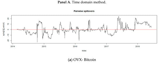
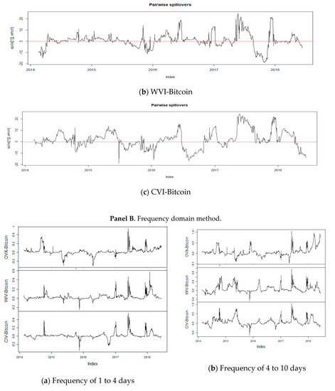
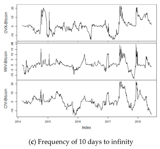
Figure 2.
Pairwise net connectedness. Panel A illustrates the pairwise net connectedness between Bitcoin and OVX, WVI, and CVI in parts (a), (b), and (c) using the time domain method, respectively. Panel B illustrates the pairwise net connectedness between Bitcoin and the three indices at three different frequencies in parts (a), (b), and (c) using the frequency domain method, respectively.
The time-domain results in Panel A show that the connectedness of all the three pairs is fluctuating but remain within the interval of 20%. In part (a), in the period from 2014 to 2016, the connectedness between OVX and Bitcoin was quite volatile due to the fluctuation of oil prices at the time. The lowest connectedness was more than negative 20%. However, in 2017, since the price of Bitcoin increased sharply, the connectedness climbed to a peak of 20% in the middle of the year and another peak at the end of 2017. Part (b) shows that the connectedness between WVI and Bitcoin was quite stable during 2014–2016. In 2017, due to the climb of Bitcoin prices, the connectedness reached its first peak in the mid-year and the second one at the year-end of around 20%. However, during 2017, since wheat prices were at lower levels than they were in the previous five years in the US, the connectedness plunged to a trough of nearly negative 20% around November. Part (c) shows the time-domain connectedness between CVI and Bitcoin. The price of corn was mainly affected by the ethanol market, crude oil prices, and climate. Therefore, the connectedness looks more volatile than that of WVI-Bitcoin in Part (b). It reached its lowest point in mid-2016 of around negative 18%, due to the downtrend in corn prices, because the corn stockpile rose more than anticipated, as a result of low feed requirements. Similar to the other two pairs, the connectedness of CVI-Bitcoin also increased during 2017, with two peaks of 20% and 18% at the middle and end of the year, respectively.
The frequency-domain results in Panel B indicate that the connectedness of the three pairs is volatile at the high frequencies of 1 to 4 days and 4 to 10 days, but fluctuates within the interval of 20% for the low frequency of 10 days to infinity. Similar to what is observed in Panel A, the connectedness of the three pairs also reached peaks at high frequencies from 1–10 days during 2017, when Bitcoin was booming. However, at the lower frequency of more than ten days, the results converge to the findings in Panel A. It shows similar patterns of the connectedness of the three pairs in Panel A, especially during 2017. These results show that there is a potential benefit of risk diversification between Bitcoin and the three commodity volatilities in the long term rather than the short term from 1 to 10 days, thanks to the connectedness range of around only 20%.
4.3. Robustness Test
Since we are interested in the hedging possibility of Bitcoin against commodity uncertainty, we will use copula functions to investigate if there is tail dependence between Bitcoin and the three commodity volatilities. The left tail dependence shows the likelihood of crashing together, whereas the right tail dependence shows the likelihood of booming together. If Bitcoin can be used as a hedger for the commodity volatilities, there should be no left tail dependence between them.
Our results, presented in Figure 3, clearly show no tail dependency between Bitcoin and the three volatility indices. This once again confirms that commodity uncertainties including corn, oil, and wheat volatilities can be effectively hedged using Bitcoin.
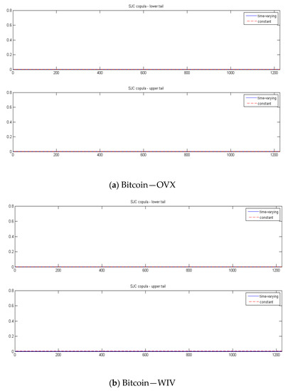
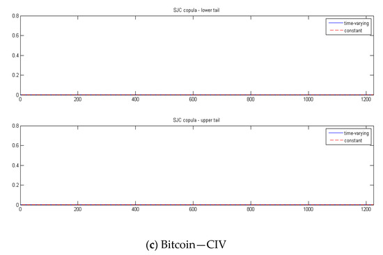
Figure 3.
Tail dependence obtained from the mixed Joe–Clayton copula. Time-varying is the time-varying tail dependence. Constant is the correlation.
5. Conclusions
This paper examines the connectedness between Bitcoin and commodity volatilities, including corn, oil, and wheat, during the period from October 2013 to June 2018, using time- and frequency-domain frameworks. The results obtained from the time-domain method show that the connectedness is 23.49%, indicating a low level of connection between Bitcoin and the three commodity volatilities. Bitcoin contributes only 2.55% to the connectedness, while the wheat volatility index accounts for 12.51% of the total connectedness. The results of the frequency-domain framework show that Bitcoin’s contribution to the total connectedness increases from high-frequency to low-frequency bands, and the total connectedness reaches up to 22.47%.
The results also indicate that Bitcoin is the spillover transmitter to the wheat volatility, while being the spillover receiver from the oil and corn volatilities. Our findings imply that the cryptocurrency of Bitcoin might be an effective hedger for commodity uncertainty, especially in the long term. The findings add further evidence into the existing Bitcoin literature that Bitcoin can also be considered as an alternative class in agriculture-product investment portfolios, rather than only in portfolios containing traditional asset classes. The results provide new insights for investors and policymakers in considering risk diversification between Bitcoin and commodities.
Author Contributions
Conceptualization, K.H. and C.C.N.; methodology, C.C.N.; data curation, C.C.N., K.H., K.P.; writing—original draft preparation, K.H., C.C.N., K.P.; writing—review and editing, T.X.N.; visualization, C.C.N. All authors have read and agreed to the published version of the manuscript.
Funding
This research received no external funding.
Conflicts of Interest
The authors declare no conflict of interest.
References
- Ardia, David, Keven Bluteau, and Maxime Rüede. 2019. Regime changes in Bitcoin GARCH volatility dynamics. Finance Research Letters 29: 266–71. [Google Scholar] [CrossRef]
- Baek, Chung, and Matthew A. Elbeck. 2015. Bitcoins as an investment or speculative vehicle? A first look. Applied Economics Letters 22: 30–34. [Google Scholar] [CrossRef]
- Bariviera, Aurelio F. 2017. The inefficiency of Bitcoin revisited: A dynamic approach. Economics Letters 161: 1–4. [Google Scholar] [CrossRef]
- Baruník, Jozef, and Tomáš Křehlík. 2018. Measuring the frequency dynamics of financial connectedness and systemic risk. Journal of Financial Econometrics 16: 271–96. [Google Scholar] [CrossRef]
- Baumöhl, Eduard. 2019. Are cryptocurrencies connected to forex? A quantile cross-spectral approach. Finance Research Letters 29: 363–72. [Google Scholar] [CrossRef]
- Baur, Dirk G., KiHoon Hong, and Adrian D. Lee. 2018. Bitcoin: Medium of exchange or speculative assets? Journal of International Financial Markets, Institutions and Money 54: 177–89. [Google Scholar] [CrossRef]
- Bianchi, Daniele. Forthcoming. Cryptocurrencies as an asset class? An empirical assessment. Journal of Alternative Investment.
- Beneki, Christina, Alexandros Koulis, Nikolaos A. Kyriazis, and Stephanos Papadamou. 2019. Investigating volatility transmission and hedging properties between Bitcoin and Ethereum. Research in International Business and Finance 48: 219–27. [Google Scholar] [CrossRef]
- Böhme, Rainer, Nicolas Christin, and Benjamin Edelman. 2015. Bitcoin: Economcis, technology, and governance. Journal of Economics Perspectives 29: 213–38. [Google Scholar] [CrossRef]
- Bouri, Elie, Georges Azzi, and Anne H. Dyhrberg. 2017a. On the return-volatility relationship in the Bitcoin market around the price crash of 2013. Economics: The Open-Access, Open-Assessment E-Journal 11: 1–16. [Google Scholar]
- Bouri, Elie, Rangan Gupta, Aviral K. Tiwari, and David Roubaud. 2017b. Does Bitcoin hedge global uncertainty? Evidence from wavelet-based quantile-in-quantile regressions. Finance Research Letters 23: 87–95. [Google Scholar] [CrossRef]
- Bouri, Elie, Peter Molnár, Georges Azzi, David Roubaud, and Lars I. Hagfors. 2017c. On the hedge and safe haven properties of Bitcoin: Is it really more than a diversifier? Finance Research Letters 20: 192–98. [Google Scholar] [CrossRef]
- Bouri, Elie, Rangan Gupta, Chi K.M. Lau, David Roubaud, and Shixuan Wang. 2018. Bitcoin and global financial stress: A copula-based approach to dependence and causality in the quantiles. The Quarterly Review of Economics and Finance 69: 297–307. [Google Scholar] [CrossRef]
- Carrick, Jon. 2016. Bitcoin as a complement to emerging market currencies. Emerging Markets Finance and Trade 52: 2321–34. [Google Scholar] [CrossRef]
- Catania, Leopoldo, Stefano Grassi, and Francesco Ravazzolo. 2019. Forecasting cryptocurrencies under model and parameter instability. International Journal of Forecasting 35: 485–501. [Google Scholar] [CrossRef]
- Chicago Board Options Exchange (CBOE). 2018. Volatility Indexes. Available online: http://www.cboe.com/products/vix-index-volatility/volatility-indexes (accessed on 20 January 2019).
- Chaim, Pedro, and Márcio P. Laurini. 2018. Volatility and return jumps in bitcoin. Economics Letters 173: 158–63. [Google Scholar] [CrossRef]
- Charles, Amélie, and Olivier Darné. 2019. Volatility estimation for Bitcoin: Replication and robustness. International Economics 157: 23–32. [Google Scholar] [CrossRef]
- Cheah, Eng-Tuck, and John Fry. 2015. Speculative bubbles in Bitcoin markets? An empirical investigation into the fundamental value of Bitcoin. Economics Letters 130: 32–36. [Google Scholar] [CrossRef]
- Ciaian, Pavel, Miroslava Rajcaniova, and d’Artis Kancs. 2016. The economics of BitCoin price formation. Applied Economics 48: 1799–815. [Google Scholar] [CrossRef]
- Corbet, Shaen, Brian Lucey, Maurice Peat, and Samuel Vigne. 2018. Bitcoin Futures—What use are they? Economics Letters 172: 23–27. [Google Scholar] [CrossRef]
- Demir, Ender, Giray Gozgor, Chi K.M. Lau, and Samuel A. Vigne. 2018. Does economic policy uncertainty predict the Bitcoin returns? An empirical investigation. Finance Research Letters 26: 145–49. [Google Scholar] [CrossRef]
- Diebold, Francis X., and Kamil Yilmaz. 2012. Better to give than to receive: Predictive directional measurement of volatility spillovers. International Journal of Forecasting 28: 57–66. [Google Scholar] [CrossRef]
- Dyhrberg, Anne H. 2016a. Bitcoin, gold and the dollar–A GARCH volatility analysis. Finance Research Letters 16: 85–92. [Google Scholar] [CrossRef]
- Dyhrberg, Anne H. 2016b. Hedging capabilities of bitcoin. Is it the virtual gold? Finance Research Letters 16: 139–44. [Google Scholar] [CrossRef]
- Feng, Wenjun, Yiming Wang, and Zhengjun Zhang. 2018. Informed trading in the Bitcoin market. Finance Research Letters 26: 63–70. [Google Scholar] [CrossRef]
- Fry, John. 2018. Booms, busts and heavy-tails: The story of Bitcoin and cryptocurrency markets? Economics Letters 171: 225–29. [Google Scholar] [CrossRef]
- Fry, John, and Eng-Tuck Cheah. 2016. Negative bubbles and shocks in cryptocurrency markets. International Review of Financial Analysis 47: 343–52. [Google Scholar] [CrossRef]
- Katsiampa, Paraskevi. 2017. Volatility estimation for Bitcoin: A comparison of GARCH models. Economics Letters 158: 3–6. [Google Scholar] [CrossRef]
- Kim, Thomas. 2017. On the transaction cost of Bitcoin. Finance Research Letters 23: 300–5. [Google Scholar] [CrossRef]
- Klein, Tony, Hien T. Pham, and Thomas Walther. 2018. Bitcoin is not the New Gold—A comparison of volatility, correlation, and portfolio performance. International Review of Financial Analysis 59: 105–16. [Google Scholar] [CrossRef]
- Koutmos, Dimitrious. 2018. Return and volatility spillovers among cryptocurrencies. Economics Letters 173: 122–27. [Google Scholar] [CrossRef]
- Kristoufek, Ladislav. 2013. BitCoin meets Google Trends and Wikipedia: Quantifying the relationship between phenomena of the Internet era. Scientific Reports 3: 3415. [Google Scholar] [CrossRef] [PubMed]
- Kyriazis, Nikolaos A. 2019. A survey on efficiency and profitable trading opportunities in cryptocurrencies markets. Journal of Risk and Financial Management 12: 67. [Google Scholar] [CrossRef]
- Kyriazis, Nikolaos A. 2020. Is Bitcoin similar to gold? An integrated overview of empirical findings. Journal of Risk and Financial Management 13: 88. [Google Scholar] [CrossRef]
- Kyriazis, Nikolaos A., Kalliopi Daskalou, Marios Arampatzis, Paraskevi Prassa, and Evangelia Papaioannou. 2019. Estimating the volatility of cryptocurrencies during bearish markets by employing GARCH models. Heliyon 5: e02239. [Google Scholar] [CrossRef]
- Mensi, Walid, Aviral Tiwari, Elie Bouri, David Roubaud, and Khamis H. Al-Yahyaee. 2017. The dependence structure across oil, wheat, and corn: A wavelet-based copula approach using implied volatility indexes. Energy Economics 66: 122–39. [Google Scholar] [CrossRef]
- Nadarajah, Sarelees, and Jeffrey Chu. 2017. On the inefficiency of Bitcoin. Economics Letters 150: 6–9. [Google Scholar] [CrossRef]
- Patton, Andrew J. 2004. On the out-of-sample importance of skewness and asymmetric dependence for asset allocation. Journal of Financial Econometrics 2: 130–68. [Google Scholar] [CrossRef]
- Pieters, Gina, and Sofia Vivanco. 2017. Financial regulations and price inconsistencies across Bitcoin markets. Information Economics and Policy 39: 1–14. [Google Scholar] [CrossRef]
- Polasik, Michal, Anna I. Piotrowska, Tomasz P. Wisniewski, Radoslaw Kotkowski, and Geoffrey Lightfoot. 2015. Price fluctuations and the use of Bitcoin: An empirical inquiry. International Journal of Electronic Commerce 20: 9–49. [Google Scholar] [CrossRef]
- Troster, Victor, Aviral K. Tiwari, Muhammad Shahbaz, and Demian N. Macedo. 2019. Bitcoin returns and risk: A general GARCH and GAS analysis. Finance Research Letters 30: 187–93. [Google Scholar] [CrossRef]
- Tiwari, Aviral K., Rabin Jana, Debojyoti Das, and David Roubaud. 2018. Informational efficiency of Bitcoin-An extension. Economics Letters 163: 106–9. [Google Scholar] [CrossRef]
- Urquhart, Andrew. 2016. The inefficiency of Bitcoin. Economics Letters 148: 80–82. [Google Scholar] [CrossRef]
- Vidal-Tomás, David, and Ana Ibañez. 2018. Semi-strong efficiency of Bitcoin. Finance Research Letters 27: 259–65. [Google Scholar] [CrossRef]
- Weber, Beat. 2016. Bitcoin and the legitimacy crisis of money. Cambridge Journal of Economics 40: 17–41. [Google Scholar] [CrossRef]
- Wu, Feng, Zhengfei Guan, and Robert J. Myers. 2011. Volatility spillover effects and cross hedging in corn and crude oil futures. Journal of Futures Markets 31: 1052–75. [Google Scholar] [CrossRef]
- Yelowitz, Aaron, and Matthew Wilson. 2015. Characteristics of Bitcoin users: an analysis of Google search data. Applied Economics Letters 22: 1030–36. [Google Scholar] [CrossRef]
© 2020 by the authors. Licensee MDPI, Basel, Switzerland. This article is an open access article distributed under the terms and conditions of the Creative Commons Attribution (CC BY) license (http://creativecommons.org/licenses/by/4.0/).