Article

Zero-Debt Policy under Asymmetric Information, Flexibility and Free Cash Flow Considerations

Department of Accountancy, Finance and Economics, Birmingham City Business School, Birmingham City University, Birmingham B5 5JU, UK
J. Risk Financial Manag. 2020, 13(12), 296; https://doi.org/10.3390/jrfm13120296
Submission received: 13 November 2020 / Accepted: 26 November 2020 / Published: 28 November 2020
(This article belongs to the Special Issue Corporate Finance, Governance, and Social Responsibility)

Abstract

:
We build a model of debt for firms with investment projects, for which flexibility and free cash flow problems are important issues. We focus on the factors that lead the firm to select the zero-debt policy. Our model provides an explanation of the so-called “zero-leverage puzzle”. It also helps to explain why zero-debt firms often pay higher dividends when compared to other firms. In addition, the model generates new empirical predictions that have not yet been tested. For example, it predicts that firms with zero-debt policy should be influenced by free cash flow considerations more than by bankruptcy cost considerations. Additionally, the choice of zero-debt policy can be used by high-quality firms to signal their quality. This is in contrast to most traditional signalling literature where debt serves as a signal of quality. The model can explain why the probability of selecting the zero-debt policy is positively correlated with profitability and investment size and negatively correlated with the tax rate. It also predicts that firms that are farther away from their target capital structures are less likely to select the zero-debt policy when compared to firms that are close to their target levels.

1. Introduction

A firm’s capital structure is one of the top issues in corporate finance theory. Over the years, financial economists have formulated and tested various theories, including trade-off theory, pecking-order theory, and market timing. Despite the tireless efforts, they remain some of the most contraversial topics in economics.
In recent years, zero-debt policy research has been an increasingly growing area of interest.1 Strebulaev and Yang (2013) call it the “zero-leverage puzzle”. The standard trade-off theory of capital structure predicts that a firm’s capital structure is the result of trade-off between the tax advantage of debt and its expected bankruptcy cost. However, this theory seems to fail to explain situations when debt is totally absent. Pecking-order theory (Myers and Majluf 1984) predicts that, under asymmetric information, firms should use internal funds before debt and debt before equity. This implies that zero-debt policy can only be adopted by financially unconstrained firms with large amounts of free cash. However, this is usually not the case (see, for example, Leary and Roberts 2005). Trade-off theory also predicts that firms should instantaneously adjust their capital structure toward their target capital structure. However, Leary and Roberts (2005) find that firms restructure their leverage infrequently.
Another interesting aspect of zero-debt firms is their dividend policy. Strebulaev and Yang (2013) find that many of these firms are dividend payers and that they pay higher dividends than other firms. Dang (2013) finds that, among zero-debt firms, there are two different groups: firms that pay dividends (consistent with Strebulaev and Yang 2013) and firms that do not. Dang (2013) argues that the latter group consists of young, unprofitable, and financially constrained firms. Strebulaev and Yang (2013) discuss the high dividends of zero-debt firms and find them quite puzzling from the points of view of traditional theories. For example, from the pecking-order theory point of view firms that are subject to asymmetric information (financially constrained firms seem to be fitting into this group) should keep their cash reserves and use them for future investments. Additionally, if firms were looking for flexibility, they would not pay dividends. In this article, we shed some new light on this issue.
As an example, consider the situation of Apple in 2012–2014. During these years Apple had no debt.2 The company’s earnings had been steadily growing between 2005–2012 and many analysts and managers, including its new CEO Tim Cook, spoke about its excessive liquidity problems (Ximénez and Sanz 2014). On 15 March 2012, CNBC confirmed that Tim Cook admitted “the company’s board of directors was actively involved in deciding what to do about the excess cash.” Secondly the company continued its growth plans and constantly faced numerous investment opportunites (Ximénez and Sanz 2014). Cook mentioned that “priorities included making as many investments as possible in research and development.” At the same time, the company started to pay dividends. Furthermore, the level of dividends was quite high (Lazonick 2017; Ximénez and Sanz 2014). A few factors are worth mentioning. As a large corporation, Apple was facing different types of agency problems, including ones arising from the ownership-management conflicts.3 The famous founder and CEO of Apple Steve Jobs, who owned a large fraction of Apple’s shares, died in 2011.4 One can assume that the company was facing a larger extent of potential agency problems, since the separation between ownership and management increased as compared to the previous period. To summarize the above discussion: Apple in 2012–2104 was a company that had no debt, paid large dividends, and faced free-cash flow and flexibility challenges.
We build a model of capital structure that contains both flexibility and free cash flow problems. Maintaining flexibility is an important incentive for firms in order to adopt a zero-leverage policy (see, for example, Dang 2013) and the free cash flow problem is one of the key factors in, for example, Byoun et al. (2013). We consider a firm with an investment project that is facing future uncertainty regarding earnings and investment size. Firms can be of three different types. If a firm does not have any financing constraints or free cash flow problems, then the first-best strategy for overcoming a potential debt overhang is to issue long-term debt. The firm would not loose any potential earnings from profitable investment opportinities in the second stage of the project.5 Another group of firms are ones that are totally constrained, in that they are not able to raise any external financing. These firms will use internal funds for financing and will not pay any dividends (keep internal cash for future investments). This is consistent with the zero-debt policy of the non-payers group in Dang (2013). However, our main focus is on the third group of firms, namely those that are partially constrained. These firms are able to raise short-term debt for financing. These firms will be dealing with potential flexibility or debt overhang problems when financing their future investment needs. In addition, firms are facing a free cash flow problem. Managerial teams can be involved in empire-building or an overinvestment problem, so a firm’s owners should take this into account when making capital structure and dividend decisions. These firms face a trade-off between the advantages of debt, including tax shield and the disciplinary advantage of limiting the free cash flow problem (Jensen 1986) and the disadvantages of debt that are related to the debt overhang problem (Myers 1977).
Our model predicts that firms that can potentially adopt the zero-debt policy are firms for which the free-cash flow problem is relatively more important than potential bankruptcy costs. These firms are more likely to pay large dividends in order to avoid free cash flow problems that are related to a manager’s overinvestment and these firms are more likely to adopt a zero-debt policy. It forces them to use more internal funds in order to finance their investments and mitigate potential free cash flow problems that are related to the accumulation of uninvested (retained) earnings. Additionally, we find that the probability of adopting the zero-debt policy increases with the expected profitability of a firm’s projects, the expected size of investments and their risk, and it decreases with tax rates. These observations are consistent with recent empirical findings (see, for example, Lotfaliei 2018). On the other hand, firms that face relatively small bankruptcy costs and a high likelihood of overinvestment by managers are not likely to adopt the zero-debt policy. They are likely to issue debt in order to provide discipline for the manager and benefit from its tax advantage. Our analysis also suggests that the choice of the zero-leverage policy can be used by high-qulaity firms to signal their quality. This is in contrast to most traditional signalling literature, such as Leland and Pyle (1977), for example, where debt serves as a signal of quality. The model also predicts that the zero-leverage policy is likely to be counter-cyclical and the positive debt policy is likely to be procyclical. It is consistent with the results of Dang (2013), Bernanke and Gertler (1989), and Kiyotaki and Moore (1997).
With regard to dividend policy, we find that zero-debt firms usually pay dividends and, in most cases, they pay higher dividends than other firms, which is consistent with Strebulaev and Yang (2013). In addition, the model generates some new predictions that have not been tested yet. For example, we find that high dividends cannot be used alone by high-quality firms as a signal of quality. This is consistent with previous literature on the dividend signalling (see, for example, Brav et al. 2005). We find that the dividend decision, together with the capital structure decision, can be used to signal a firm’s quality. For example, a separating equilibrium may exist where the high-quality firm uses zero-debt policy and pays high dividends and the low-quality firm uses positive debt policy and pays a smaller dividend. The low-quality firm will not mimick the high-quality firm, since the potential benefits from mitigating the debt overhang problem are not as valuable for this firm as they are for a high-growth firm, since it has a smaller expected investment project size and lower expected payoffs in the second stage of the project. Accordingly, unlike the high-growth firm, these benefits for the low-growth firm can be outweighed by tax shield losses. Bessler et al. (2013) find that zero-debt firms have positive abnormal return as compared to their peers, which is consistent with our result.
The model also predicts that the likelihood of selecting the zero-debt policy is different for different types of firms. Underleveraged firms that are far from their target capital structures are less likely to drop the zero-debt policy when compared to firms that are close to their target levels. A similar result was found in Leary and Roberts (2005), who used an adjustment cost argument (see also Warr et al. 2012). Note that the adjustment cost approach has been questioned in recent literature (see, for example, Lambrinoudakis 2016).
Lotfaliei (2018) extends trade-off theory by including a real option to wait before issuing debt. This can induce a zero leverage, even when standard trade-off theory predicts that these firms should have leverage. The real option’s effect is similar to that of bankruptcy costs. The value of firms with no debt include the option whose value is derived from future debt benefits and reduced bankruptcy costs. This article proposes a model that determines the optimal timing for the aquisition and sale of debt and finds support for its predictions through simulations and empirical analysis. Unlike our paper, it does not reach any closed solutions or propositions regarding the zero-debt policy. Most of their results are obtained via simulations using different numerical assumptions and shapes of different functions, in particular the non-convexity of debt costs, which are crucial for their results.6
Our paper is one of the first that analyzes debt policy under the debt overhang and free cash problems simultaneously. Hart and Moore (1994) analyze a model with long-term debt, where managers have both an incentive to overinvest (similar to the free cash flow problem) and underinvest (debt overhang). They argue that a company with high debt will find it hard to raise capital, since new security holders will have low priority relative to existing creditors. Conversely, they show that, for a company with low debt, there is an optimal debt-equity ratio and mix of senior and junior debt if management undertakes unprofitable as well as profitable investments. In contrast to our paper, the zero-debt policy only emerges for risk-free high profitable firms, which is not consistent with recent empirical evidence. Hirth and Uhrig-Homburg (2010) examine the effect of overinvestment and underinvestment problems on a firm’s cash flow and capital structure decisions in a continuous-time framework. In contrast to our paper, the overinvestment problem is modelled as an asset substitution problem. They show that stockholder–bondholder agency conflicts cause investment thresholds to be U-shaped in leverage and decreasing in liquidity. The paper shows that an interior solution for liquidity and capital structure optimally trades off tax benefits and agency costs of debt. The zero-debt policy does not emerge in equilibrium.
The rest of the paper is organized, as follows. Section 2 contains a literature review. Section 3 presents the model and its main results. Section 4 analyzes the factors that affect the probability of selecting/dropping the zero-debt policy and it also provides a comparative static analysis regarding zero-debt firms and dividend-paying/non-paying firms. Section 5 presents a variation of the model with asymmetric information. Section 6 presents the model’s implications and its consistency with empirical evidence. Section 7 discusses the model’s robustness and extensions and Section 8 concludes.

2. Literature Review

2.1. Debt Overhang

The debt overhang problem occurs when firms do not invest in projects with positive net present values (NPVs). Equityholders may pass up profitable investments, because the firm’s existing debtholders capture most of benefits from the project (Myers 1977). This is because the NPV of a project is sometimes different for shareholders and creditors. A firm will choose projects with the highest earnings for shareholders if the managers act in the interest of the shareholders. The problem is that projects with positive NPVs (for the firm as a whole) sometimes have low payoffs to the shareholders if the firm’s debt is large enough. Debt has priority over equity in cases when earnings are not sufficient for satisfying every claimholder.
Some notable papers include the following. Gertner and Scharfstein (1991) show that, conditional on ex-post financial distress, making a fixed promised debt payment due earlier (i.e., shorter-term) raises the market value of the debt and, thus, the firm’s market leverage, leading to more debt overhang. Diamond (1991) argues that firms build their reputaion in order to raise their credit rating and improve their ability to issue debt. Similar to our paper, it focuses on financially constrained firms that are not able to issue long-term debt. However, zero-debt policy is not considered in this paper. In contrast, our model includes both debt overhang and free cash flow considerations. Diamond and He (2014) compare short-term debt and long-term debt with regard to potential debt overhang problems.7
Overall theoretical literature on debt overhang has failed to recongnize opportunities to combine debt overhang and free cash flow ideas in order to generate zero-debt results. The closest paper, in this sense, to ours is Berkovich and Kim (1990). They combine the underinvestment (debt overhang) and overinvestment problems in order to generate predictions regarding debt covenants and debt seniority. However, in their article, overinvestment has the form of an asset substitution problem (Jensen and Meckling 1976) and not a free cash flow problem (as in our paper) and the zero-debt policy is not explained.

Flexibility Theory of Capital Structure

We cover flexibility theory in a separate subsection of the debt overhang section, since there is still debate regarding whether or not this theory represents a separate theoretical idea from the debt overhang idea. Firms in the development stage need financial flexibility. There is a lot of uncertainty, because they consider a lot of investment projects, including their financing strategies, which requires a lot of flexibility. Having too much debt in capital structure will not help here (similar to a debt overhang problem). In addition, firms in the development stage likely do not have a favorable track record (i.e., credit ratings) of borrowing (Diamond 1991) and they are most likely to be turned down for credit when they need it most. Mature firms, for the most part, generate positive earnings and have more financial flexibility than developing firms. Accordingly, these firms rely more on debt financing for funding their investments, as they face less financing constraints, in that they expect to repay their debt with future earnings.
Flexibility theory finds a lot of support in empirical studies (Byoun 2011) and manager surveys (Graham and Harvey 2001). Gamba and Triantis (2008) develop a theoretical model that analyzes optimal capital structure policy for a firm that values flexibility in the presence of personal taxes and transaction costs. Among recent papers, note Sundaresan et al. (2015), who analyze a growing firm that represents a collection of growth options and assets in place. The firm trades off tax benefits with the potential financial distress and endogenous debt overhang costs over its life cycle. The authors argue that the firm consistently chooses conservative leverage in order to mitigate the debt-overhang effect on exercising decisions for future growth options.
Like debt overhang literature, flexibility theory literature does not provide a good understanding of facts that are related to the zero-debt policy. The importance of financial flexibility, as compared to major theories of capital structure, remains an open question. More work that compares flexibility theory with other theories is expected.

2.2. Free Cash Flow Theory

Grossman and Hart (1982) and Jensen (1986) argue that the use of debt financing can be used in order to mitigate the tendency for “empire-building”. Jensen (1986, 1989) argued that debt financing is an effective way to resolve agency problems between managers and investors: It would limit managerial discretion by minimizing the “free cash-flow” available to managers and, thus, provide protection to investors. Sometimes in literature, this idea is referred to as “debt and discipline” theory.8
As we know, using debt as a major source of financing incurs substantial costs of financial distress. Firms may face direct bankruptcy costs or indirect costs in the form of debt-overhang or asset substitution. In order to reduce the risk of financial distress, it may be desirable to have the firm rely partly on equity financing.
DeMarzo and Fishman (2007) consider a dynamic model where a firm’s manager can divert the firm’s cash flow. It is shown that an optimal mechanism can be implemented by combining equity, long-term debt, and a line of credit. Zhang (2009) analyzes the effect of a firm’s capital structure on managerial incentives and controlling the free cash flow agency problem and compares it to incentives that are provided by compensation contracts. It was found that debt and executive stock options act as substitutes in attenuating a firm’s free cash flow problem. Edmans (2011) suggests that the option to terminate a manager minimizes the investors’ losses early if the manager is unskilled. It also deters a skilled manager from undertaking efficient long-term projects that risk low short-term earnings. This paper demonstrates how risky debt can overcome this tension.
Our paper adds the dividend policy choice and the debt overhang problem to a typical free cash flow model. In such an environment, firms can select between debt as a disciplinary device to mitigate the free cash flow problem as in traditional literature and another policy that includes zero debt and high dividends.9

2.3. Signalling under Asymmetric Information

Information asymmetries are characterized by one entity having more information than another. Insiders may have private (exclusive) information about a firm that is unavailable to outsiders. Not knowing for sure what the firm is worth, outside investors will not be willing to pay much for its newly issued equity. Therefore, if the firm is actually good, then its equity will be underpriced. Because of this, a good firm should always rely on retained earnings in order to finance new projects. These ideas were put forth by Myers (1984) and Myers and Majluf (1984). High-quality firms will use internal funds first and, in their absence, will issue debt and only as a last resort will issue equity (so called pecking order). Risky debt also suffers from asymmetric information problems (for example, in the form of higher interest rates for firms), but not to the same degree as equity underpricing.
The empirical evidence regarding whether firms follow the pecking order is mixed, as mentioned in Miglo (2011). The negative reaction to equity issues, or, in general, to leverage reducing transactions, usually finds empirical support. The evidence regarding the link between the extent of asymmetric information and capital structure choice and regarding the pecking order is mixed.
The signalling theory of capital structure offers models in which capital structure serves as a signal of private information (Ross 1977; Leland and Pyle 1977). Usually, in these models, the market reaction on debt issues is positive. Empirical evidence is mixed regarding the predictions of signaling theory.
Finally, consider the signalling theory of dividends. It suggests that, if a company announces a decrease/increase in dividend payouts, it can be interpreted as a signal of negative/positive future prospects of the company.
Bhattacharya’s (1979) model assumes that external investors do not have full information regarding a company’s expected cash flows. The findings claim that the dividends contain information about present and prospective cash flows and, for that reason, they can be used by managers as signals to help close the information gap. Miller and Rock (1985) consider both dividend and investment policies. They argue that a struggling company may raise dividend payments to a level where investors would assume that the firm is financially good and, consequently, pay a higher amount for its shares. A stronger company might have to compete by raising its dividends beyond what the struggling company can match. The Williams (1987) model helps to explain why some companies aim to both raise capital and distribute dividends at the same time. It also suggests that firms with more “valuable” internal information tend to distribute higher dividends.
Lee and Ryan (2002) analyse dividend signalling theory and the relationship between earnings and dividends. They conclude that free cash flow and recent performance mostly influence the dividend payment strategy. Benartzi et al. (1997) argue that dividends do not signal future performance, but reflect past performance. Recent empirical literature finds mixed evidence regarding signalling theories of dividends (Brav et al. 2005).
All of the above presented studies try to answer the question of whether dividends have any signalling power and affect the share price. In spite of numerous articles and studies, the issue of whether dividend announcements contain information is still unclear and no consensus has been reached. Our paper contrbutes to this literature by suggesting that dividends can be used, together with capital structure, in order to signal a firm’s quality.

3. The Model and Basic Results

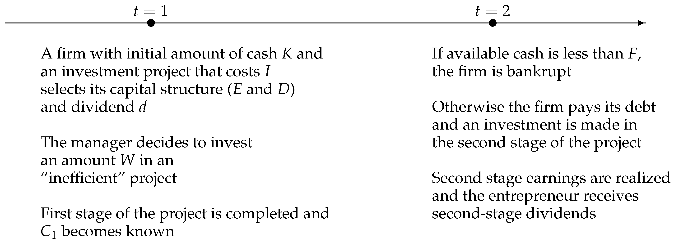
3.1. Model Description

Debt overhang/Flexibility theory suggest that, if a firm has too much debt, then it will be harder for them to obtain loans when necessary (Myers 1977). Therefore, firms preserve debt capacity or hold back on issuing debt, because they want to maintain flexibility. Firms maintain excess debt capacity or larger cash balances than warranted by current needs, in order to meet unexpected future requirements. While maintaining financial flexibility has value to firms, it also has a cost; excess debt capacity implies that a firm is giving up some value (e.g., tax benefit of debt) and it has a higher cost of capital.
Free cash flow theory (Jensen 1986) suggests that managers have a tendency to overinvest if the threat of bankruptcy is not high enough (empire-building). This moral hazard problem can be mitigated if the firm uses debt as a disciplinary device. If a manager spends funds inefficiently, then the firm will not be able to generate enough cash to cover their existing debt and the probability of bankruptcy will increase. In this case, the probability of losing a job for managers increases (Hoskisson et al. 2017). As an alternative to issuing debt, the firm can increase dividends to shareholders. This will also reduce the amount of available free cash (Brav et al. 2005).
Some basic ideas can be illustrated by the following model. Consider a firm that exists for two periods T = 1 , 2 . Initially, the firm has cash K. The firm also has an investment project. The project requires an amount of investment I and it can generate cash flows, as follows. First, it brings an amount C 1 , which can later be invested (second stage) with the average rate of return r. I and K are known, while C 1 is risky. It is uniformly distributed between 0 and C 1 ¯ .10 We also assume that C 1 ¯ / 2 > I and r > 0 , which implies that both stages of the project have a positive net present value. The firm belongs to the shareholders who we will call the entrepreneur. The entrepreneur is responsible for making capital structure and dividend decisions. In order to finance the initial investment I, the firm can either use internal funds (E) or issue debt (D), I = E + D .11
Debt that is issued to finance the project should be paid back at T = 2 . Let F be the face value of the debt (including principal and interest), due to, at the time, that the investment in the second stage of the project must be made ( T = 2 ).12 The firm is financially constrained and it is not able to issue a long-term debt, i.e., debt due upon the completion of the second stage of the project. Hence, the firm is facing a potential debt overhang or flexibility loss problem. A high amount of debt limits the firm’s investment capacity. If F > C (C denotes available cash before the second stage of the investment project), then the firm will not be able to make any investments and, if F < C , the firm can make a full or partial investment in the second stage of the project.13 A disadvantage of having low debt is that it can reduce, for example, the amount of tax shield, and ultimately increase the cost of capital and, respectively, reduce the value of the firm. This approach is consistent with Graham (2000) and Strebulaev and Yang (2013), who suggest that zero-debt firms seemingly do not use any substitutes for debt that provide similar advantages as leases for example. Let F * be the maximal amount of debt that the firm can issue.14 We assume that F * C 1 ¯ . This allows for us to model a large spectrum of possible financing strategies from 100% internal funds to 100% debt.15
In addition, the firm faces a free cash flow problem. During the first stage of the project (before C 1 becomes known), the firm’s managerial team (call it the manager) has an opportunity to invest the firm’s funds in an “inefficient” project that does not increase the firm’s value, but instead can provide private benefits for the manager. The manager cannot be perfecty monitored by the entrepreneur (in the spirit of Grossman and Hart 1982 or Jensen 1986). We assume that, if the manager decides to invest an amount X of the firm’s available cash in an “inefficient” project, he gets a X , 0 a 1 . The firm gets nothing and it just loses an amount X in this case. The manager is also bankruptcy averse. When deciding whether to make an inefficient investment, the manager faces a trade-off between receiving private benefits and reducing disutility from increasing the bankruptcy risk of the firm. When investing in an “inefficient” project, the manager consequently increases the chances of the firm going bankrupt. If this is the case, the manager’s disutility is B , B 0 (job loss, reputation loss, family values, etc.).16
When choosing the amount of debt, the firm faces a trade-off between the flexibility, free cash flow, and cost of capital minimization problems. When debt equals F, the value that is created by minimizing the cost of capital (in absolute values for shareholders; analogous, for example, to the present value of the tax shield) equals F t , 0 t 1 for any F F * .17 Everybody is risk-neutral and the risk-free interest rate is zero. Figure 1 presents the timing of events.

3.2. No Free Cash Flow Problem and No Financial Constraints

Let us first consider a perfect market case when the firm does not face any free cash flow problems and no financial constraints exist. More specifically, we assume that the manager is totally honest and does not make any inefficient investments in private projects and that the firm can issue long-term debt.18 This assumption assures that a debt overhang problem does not arise. Consequently, the firm will not lose any potential earnings from the second stage of the project given that r > 0 , because the firm can invest the full amount of available cash in the second stage of the project. Under these conditions, the amount of debt issued by the firm as well as its dividend policy is irrelevant (Modigliani and Miller 1958). If taxes are introduced in the model, then the optimal policy is to select F = F * . This policy minimizes the cost of capital and maximizes the investment return. The creditors will be happy to provide a long-term loan with a face value F, such that
D = F F 2 2 C 1 ¯ ( 1 + r )
Indeed, even if the firm paid the highest possible dividend K ( I D ) at T = 1 , the expected payment to the creditors (recall that C 1 is uniformly distributed) equals
C 1 ¯ ( 1 + r ) F C 1 ¯ ( 1 + r ) F + F 2 2 C 1 ¯ ( 1 + r )
Here, C 1 ¯ ( 1 + r ) F C 1 ¯ ( 1 + r ) is the probability that C 1 ( 1 + r ) F and that debt can be paid in totallity. Respectively, F C 1 ¯ ( 1 + r ) is the probability that C 1 ( 1 + r ) < F and F 2 is the average amount that the creditors will receive when C 1 ( 1 + r ) < F . One can see that (1) equals (2). The firm’s expected value is
d + K ( I D ) d + C 1 ¯ ( 1 + r ) F C 1 ¯ ( 1 + r ) ( C 1 ¯ ( 1 + r ) + F 2 F )
Here, d is the dividend paid to the entrepreneur at T = 1 ; K ( I D ) d is the amount of retained earnings at the beginning of T = 2 and C 1 ¯ ( 1 + r ) + F 2 is the average value of C 1 ( 1 + r ) for the case when C 1 ( 1 + r ) F . While using (2), we can write (3) as
K I + C 1 ¯ 2 ( 1 + r )
Therefore, without taxes, both the capital structure and dividend policy are irrelevant, because (4) does not depend on D, F or d. If t > 0 , the optimal debt is F = F * and the firm’s value equals K I + C 1 ¯ 2 ( 1 + r ) + F * t . Now, consider the case with a free cash flow problem and financial constraints.

3.3. Financially Constraint Firm with Free Cash Flow Problem

3.3.1. Manager’s Decision at the End of T = 1

Consider the manager’s decision at the end of T = 1 . Let C 0 be the amount of retained earnings (after the firm pays dividends) at T = 1 and R be the amount of cash that will be left if the manager withdraws W , W + R = C 0 . Three cases are possible. (1) R F . In this case, the firm can pay back its debt and the manager’s utility is a W = a ( C 0 R ) . Because it is decreasing in R, the optimal R = F and the manager’s expected utility E ( U ) is a ( C 0 F ) (2).
C 0 F > R
When making a decision, the manager does not know the value of C 1 . Depending on the future realization of C 1 , two situations may exist. 1. C 1 F R . In this case, the firm can pay back its debt and the manager’s utility is a ( C 0 R ) . 2. C 1 < F R . In this case, the firm will be bankrupt at the end of T = 2 and the manager’s overall utility is a ( C 0 R ) B . The probability that C 1 F R equals C 1 ¯ F + R C 1 ¯ and the probability that C 1 < F R equals F R C 1 ¯ . Hence, the expected value of the manager’s utility E ( U ) equals
a ( C 0 R ) ( F R ) C 1 ¯ B
The manager’s choice of W and respectively R is determined by maximizing E ( U ) . Note that (6) is linear in R, so R = 0 if a > B C 1 ¯ and otherwise R should be maximized (if a = B C 1 ¯ , the manager is indifferent between his options. For simplicity, we assume that, in this case, the manager will not bankrupt the firm).
It follows from the above analysis (note that, in both cases, C 0 F ) that if a B C 1 ¯ , the optimal R = F . Otherwise, the optimal R = 0 .
(3) C 0 < F . Similarly to the analysis in the previous case, we find that the expected value of the manager’s utility equals a ( C 0 R ) F R C 1 ¯ B . We have R = 0 if a > B C 1 ¯ and R = C 0 otherwise.
This leads to the following lemma.
Lemma 1.
(1) C 0 F . Then R = 0 if a > B C 1 ¯ and R = F otherwise. (2) C 0 < F . Then R = 0 if a > B C 1 ¯ and R = C 0 otherwise.
Proof. 
Follows from the the above analysis. □
The interpretation of Lemma 1 is following. If the bankruptcy cost is more important for the manager than private benefits from overinvestments (i.e., B is relatively higher than a), the optimal decision for the manager is to keep cash in the firm. Otherwise, the manager will make a lot of inefficient investments and receive a large amount of private benefits.

3.3.2. Entrepreneur’s Dividend Decision at T = 1

Although the capital structure and dividend decisions are made simultaneously (e.g., during the shareholder meeting), we will first calculate the optimal dividend policy for any arbitrarily chosen capital structure and then we will analyze the optimal capital structure choice. We have R 0 = d + C 0 , where
R 0 = K ( I D )
is the amount of funds available after the firm’s capital structure was determined, including the amount of retained earnings used to finance the initial stage of the project ( I D ).
Proposition 1.
(1) If a B C 1 ¯ , d = R 0 ; (2) if a < B C 1 ¯ , d = R 0 F when R 0 > F and F < 2 C 1 ¯ r 1 + r ; d = R 0 when R 0 > F > 2 C 1 ¯ r 1 + r or when F > R 0 and F > R 0 2 + C 1 ¯ r 1 + r ; and d = 0 otherwise.
Proof. 
Two cases are possible.
(1) a < B / C 1 ¯ . In turn, three situations may exist. 1. R 0 d F . As follows from Lemma 1, the manager will “steal” R 0 d F , so the remaining amount of retained earnings F will be used in order to pay back debt at T = 2 . The firm can invest the full amount that is required for the second stage of the project and the firm’s value equals
d + C 1 ¯ 2 ( 1 + r ) + F t
Because (8) is increasing in d, the optimal d = R 0 F . The firm’s value equals R 0 F + C 1 ¯ 2 ( 1 + r ) + F t .
2. F < R 0 < F + d . Because C 0 = R 0 d < F , Lemma 1 implies that, in this case, R = C 0 = R 0 d . The firm is not able to make a full amount of investment for the second stage of the project. If C 1 F ( R 0 d ) , then the firm can still make a partial investment. Because of the probability that C 1 F R 0 + d equals C 1 ¯ F + R 0 d C 1 ¯ , the firm’s expected value equals:
d + C 1 ¯ F + R 0 d C 1 ¯ ( R 0 d + C 1 ¯ + F R 0 + d 2 F ) ( 1 + r ) + F t
Because (9) is convex in d, possible solutions are either d = R 0 F or d = R 0 . According to (9), if d = R 0 F , the firm’s expected value equals R 0 F + C 1 ¯ 2 ( 1 + r ) + F t . If d = R 0 , E ( V ) = R 0 + ( C 1 ¯ F ) 2 2 C 1 ¯ ( 1 + r ) + F t . Proposition 1, for the case a < B C 1 ¯ and F < R 0 , follows from the comparison of the above expressions, i.e., d = R 0 F is better if F < 2 C 1 ¯ r 1 + r and, otherwise, d = R 0 is the best strategy.
3. R 0 < F . Note that, in this case, R 0 d < F . Additionally, note that Lemma 1 implies R = C 0 . Similarly to the previous case, we find that the firm’s expected value is as in (9). This time, the possible solutions are either d = 0 or d = R 0 . According to (9), if d = 0 ,
E ( V ) = ( C 1 ¯ ( F R 0 ) ) 2 2 C 1 ¯ ( 1 + r ) + F t
If d = R 0 ,
E ( V ) = R 0 + ( C 1 ¯ F ) 2 2 C 1 ¯ ( 1 + r ) + F t
The comparison of (10) and (11) reveals that the latter is greater if
F > R 0 2 + C 1 ¯ r 1 + r
(2) a B / C 1 ¯ . Note that, according to Lemma 1, in this case R = 0 and also that C 1 F C 1 . The latter implies that, as long as F > 0 , a full investment in the second stage is not possible. Two cases are possible. 1. C 1 F . In this case, the firm can make a partial investment and the firm’s value equals d + ( C 1 F ) ( 1 + r ) + F t . 2. C 1 < F . In this case, the firm is not able to make any investments in the second stage of the project and the firm’s value to the entrepreneur is d + F t . □
Next, we need to calculate the expected change in the firm’s value. The probability that C 1 > F equals ( C 1 ¯ F ) / C 1 ¯ and the average amount of investment needs is ( F + C 1 ¯ ) / 2 . Hence, the expected firm’s value E ( V ) equals
d + ( C 1 ¯ F ) C 1 ¯ ( F + C 1 ¯ 2 F ) ( 1 + r ) + F t
Because (12) is increasing in d, the optimal solution is d = R 0 .
The interpretation of Proposition 1 is as follows. If the entrepreneur expects the manager to overinvest, then he will pay a high dividend. Otherwise, some funds can be kept inside the firm.

3.3.3. Entrepreneur’s Capital Structure Decision at T = 1

Proposition 2.
When a B C 1 ¯ , F = 0 if r 3 2 t or r < 3 2 t and F * < 2 C 1 ¯ ( r t ) r . Otherwise, F = F * .
Proof. 
Let a B / C 1 ¯ . In this case, as follows from Proposition 1, d = K ( I D ) and R = 0 . The firm’s value equals K I + D + C 1 ¯ F C 1 ¯ ( F + C 1 ¯ 2 F ) ( 1 + r ) + F t . The creditors will be paid in full when C 1 > F and they will receive C 1 otherwise. Therefore: D = C 1 ¯ F C 1 ¯ F + F C 1 ¯ F / 2 = F F 2 2 C 1 ¯ . Hence, the firm’s value equals
K I + F F 2 2 C 1 ¯ + C 1 ¯ F C 1 ¯ ( F + C 1 ¯ 2 F ) ( 1 + r ) + F t
Because (13) is convex, the possible solutions are either F = 0 or F = F * . According to (13), if F = 0 ,
E ( V ) = K I + C 1 ¯ ( 1 + r ) 2
If F = F * , E ( V ) = K I + F * F 2 2 C 1 ¯ + ( C 1 ¯ F * ) 2 2 C 1 ¯ ( 1 + r ) + F * t = K I F * r + ( F * ) 2 2 C 1 ¯ r + C 1 ¯ ( 1 + r ) 2 + F * t . Proposition 2 follows from the comparison of this expression with (14), i.e., it follows that F = 0 if
F * 2 C 1 ¯ ( r t ) r
and F = F * otherwise. Note that the right side of (15) is greater than C 1 ¯ if
r 3 2 t
In this case, F = 0 , because F * C 1 ¯ 2 C 1 ¯ ( r t ) r . □
Proposition 3.
If a < B C 1 ¯ and t is sufficiently small, the optimal amount of debt increases with C 1 ¯ and r.
Proof. 
See Appendix A. □
Two points from the proof of Proposition 3 are discussed below. First, if
R 0 F
the optimal amount of debt is either F = 2 C 1 ¯ r 1 + r or F = F * . Also in this case d = 0 .
Second, we present an example (for simplicity, we consider the case K = I , r < 1 and t is marginally small) of the link between optimal debt and C 1 ¯ . Let C * = ( 1 + r ) F * 2 r . Subsequently, we find that F = F * if C 1 ¯ > C * ; and, F = 2 C 1 ¯ r 1 + r if C 1 ¯ < C * .
The results of Proposition 3 regarding C 1 ¯ and r are interesting and opposite to the results of Proposition 2. In the case that the manager is less likely “to steal” money from the firm ( a < B C 1 ¯ ), the entrepreneur may be interested to keep cash for the second period and, hence, use more debt to finance the first stage of the project. The higher the expected size of the potential investment in the second stage the higher the amount of debt that is issued by the firm. For example, it follows from Figure 2 that =m when C 1 ¯ is high, the firm uses as much debt as possible ( F * ). Otherwise, it is a trade-off between the advatages and disadvatges of debt. If C 1 ¯ is really small, then the firm will issue a smaller amount of debt.
Our focus is on firms with the zero-leverage policy and factors that lead to this policy. The comparative static analysis reveals the following.

4. Comparative Statics

Corollary 1.
An increase in the expected performance of a firm’s projects increases its chances of selecting the zero-debt policy. An increase in the uncertainty about future projects/size of investments also increases the chances of selecting this policy. An increase in the tax rate decreases the chances of selecting the zero-debt policy.
An increase in r in (15) increases the chances that D = 0 . It is the potential return that the firm earns on its projects that provides the value to flexibility. Other things remaining equal, firms operating in businesses where projects earn substantially higher returns than their hurdle rates should value flexibility more than those that operate in stable businesses where the excess returns are small.
An increase in C 1 ¯ in (15) also increases the chances that D = 0 . If flexibility is viewed as an option, then its value will increase when there is greater uncertainty regarding future projects; thus, firms with predictable capital expenditures should value flexibility less.
An increase in t in (15) increases the chances that F = F * . Debt should be high when a firm has high profit and uses leverage to reduce taxes, or when potential bankruptcy costs are relatively low and the cost of debt remains relatively low, regardless of the level of debt or when the cost of equity remains significantly higher relative to the cost of debt (for example, due to the situation in the stock market) when debt is low. Those firms should value flexibility less.
Corollary 2.
Non-dividend-paying firms are as follows: (1) managers do not steal money; (2) debt is relatively high; and, (3) free cash is relatively small.
The only case when firms do not pay dividends is when a < B / C 1 ¯ and condition (17) holds. The former means that, in this case, the manager steals less funds from the company when compared to the case when a B / C 1 ¯ . The latter means that R 0 = K I + D is relatively small. Other things being equal, it implies that free cash (K) should be relatively small in order for (17) to hold. Finally, these firms take maximal debt and benefit from its tax advantages.
Corollary 3.
Dividend paying zero-leverage firms (ZLPD) differ from dividend paying non-zero leverage firms (NZPD) in that: (1) for ZLPD free-cash flow problems are more important than bankruptcy costs; and, (2) ZLPD pay higher dividends.
With regard to the first point note that, for ZLPD, we have a B / C 1 ¯ . With regard to the second point note that ZLPD pay the entire amount of retained earnings available as dividends. For NZPD, different cases can emerge. In most cases, they keep some cash inside the firm. Hence, on average, ZLPD pays higher dividends than NZPD.
So far, our focus has been on the role of r, t and C 1 ¯ . Now, consider the role of F * for zero-debt policy decisions. Consider two firms with F 1 * and F 2 * , such that
F 1 * < F 2 *
Condition (15) predicts that Firm 2 is less likely to select the zero-leverage policy than Firm 1.
Corollary 4.
The firm with F 2 * is less likely to select the zero-debt policy than the firm with F 1 * .
The proof follows directly from (15) and that F 1 * < F 2 * .
One can assume that F * is connected to the term target debt ratio. This term is usually used in literature with regard to traditional static trade-off theory. In our model, as was argued in Section 3.2, this is an optimal amount of debt for a firm that does not face any free cash flow or flexibility problems, etc. In this case, Corollary 4 has an interesting empirical interpretation. If both firms have no debt initially (by the time the decisions should be made), condition (18) means that Firm 1 is closer to its target ratio than Firm 2. Therefore, Corollary 4 means that the firm that is farther from its target debt level is less likely to select the zero-debt policy.

5. Asymmetric Information about Firm’s Investment Opportunities/Performance

Now, suppose that information regarding the firm’s performance is asymmetric. More specifically, let us assume that there are two types of firms. The maximal profit for the stage 1 investment for type 1 equals C 1 ¯ and, for type 2, it equals C 2 ¯ , C 1 ¯ < C 2 ¯ .

5.1. Separating Equilibrium

An equilibrium is defined as a situation where no firm type has an incentive to deviate. A separating equilibrium is one where firms select different strategies. We will also check that the off-equilibrium beliefs of market participants survive the intuitive criterion of Cho and Kreps (1987). This condition means that the market off-equilibrium beliefs are reasonable in the sense that, if, for any firm type, its maximal payoff from deviation is not greater than its equilibrium payoff, then the market should place a probability of 0 on possible deviations of this type. The above definitions are consistent with the standard perfect bayesian equilibrium definition (see, for instance, Fudenberg and Tirole 1991) with the addition of an intuitive criterion, which is quite common in these types of games (see, for instance, Nachman and Noe 1994).
The idea is that a firm with better growth opportunities (higher C 1 ¯ ) may select the zero-debt policy as a signal of growth. Indeed, low-growth opportunity firms may find it unprofitable to mimick this strategy, because it limits its investment opportunities in the second stage and no gain is achieved from reaching lower interest rates. In contrast, if the high-growth firm selects a positive debt strategy, then it will be mimicked by the low-qaulity firm, because of the opportunities in obtaining a loan with a lower interest rate.
Proposition 4.
There is no separating equilibrium where firms select different levels of debt and pay the same amount of dividends; there is no separating equilibrium where firms selects the same level of debt and pay different amounts of dividends.
Proof. 
See Appendix A. □
For the first part, the idea is simply that, in this case, the low-quality firm will be able to either mimick the high-quality firm and obtain a low interest rate (in case the high-quality firm has positive debt) or increase dividends if the high-quality firm does not issue debt and, thus, could not pay a high dividend. As follows from (7), the firm that issued more debt will be able to save more internal funds and, therefore, pay a higher dividend. For the second part, if firms use the same amount of debt, then they should have similar preferences for dividends, as follows from Propositions 1–3. Therefore, one of the firms will eventually deviate by selecting a dividend amount different from its equilibrium value.
Proposition 5.
There exists a separating equilibrium where type 2 selects F 2 = 0 and d 2 > 0 and type 1 selects F 1 > 0 and d 1 d 2 . A separating equilibrium, where type 2 selects F 2 > 0 and type 1 selects F 1 such that F 2 > F 1 does not exist.
Proof. 
See Appendix A. □
To illustrate the proposition, suppose
a > B C 1 ¯ > B C 2 ¯
2 C 1 ¯ ( r t ) r < F * < 2 C 2 ¯ ( r t ) r
Additionally, suppose that type 2 selects F 2 = 0 and d 2 = K I and Type 1 selects F 1 = F * and d 1 = K I + F * . Note that (19) implies that the strategies of the firms correspond to the optimal symmetric information strategies described by Propositions 1 and 2. Equilibrium payoffs are: type 2 – K I + C 2 ¯ ( 1 + r ) 2 ; type 1 –
K I + F * ( F * ) 2 2 C 1 ¯ + ( C 1 ¯ F * ) 2 2 C 1 ¯ ( 1 + r ) + F * t
If type 2 deviates and mimicks type 1, then it will have to borrow with a higher interest rate that correpsonds to type 1: D = F * ( F * ) 2 2 C 1 ¯ . Hence, its profit will be K I + F * ( F * ) 2 2 C 1 ¯ + ( C 2 ¯ F * ) 2 2 C 2 ¯ ( 1 + r ) + F * t . This is less than K I + F * ( F * ) 2 2 C 2 ¯ + ( C 2 ¯ F * ) 2 2 C 2 ¯ ( 1 + r ) + F * t , which is, in turn, less than K I + C 2 ¯ ( 1 + r ) 2 , because F * < 2 C 2 ¯ ( r t ) r . If type 1 deviates, its payoff is K I + C 1 ¯ ( 1 + r ) 2 , which is smaller than K I + F * ( F * ) 2 2 C 1 ¯ + ( C 1 ¯ F * ) 2 2 C 1 ¯ ( 1 + r ) + F * t because 2 C 1 ¯ ( r t ) r < F * . Accordingly, this equilibrium exists.
Proposition 5 implies that the high-quality firm selects zero-debt policy and a high level of dividend in order to efffectively signal its quality.

5.2. Pooling Equilibrium

Next, we analyze the pooling equilibria. We define a pooling equilbrium as one where both types of firms select the same strategy. If multiple pooling equiliria exist, then we will use the mispricing criterion to evaluate which one is most likely to exist. We use the standard concept of mispricing that can be found, for example, in Nachman and Noe (1994). The magnitude of mispricing in a given equilibrium is equal to that of undervalued type(s). The overvaluation of overvalued type(s) does not matter.
Proposition 6.
Pooling with F = 0 exists if a > B C 1 ¯ > B C 2 ¯ and F * < 2 C 1 ¯ ( r t ) r < 2 C 2 ¯ ( r t ) r . Pooling with F > 0 exists if 2 C 1 ¯ ( r t ) r < 2 C 2 ¯ ( r t ) r < F * and x is sufficiently large.
Proof. 
See Appendix A. □
In Proposition 6, we find that pooling with no debt exists as long as the conditions of optimality for the zero-debt policy under symmetric information ( F * < 2 C 1 ¯ ( r t ) r < 2 C 2 ¯ ( r t ) r ) hold for both types. This is because there is no adverse selection game with the value of debt (interest rate) for the low-quality type, since no type issues any debt in equilibrium. An equilibrium with positive debt only exists if the fraction of high-quality firms is sufficiently high. Respectively, the interest rate is sufficiently low and the high-quality types do not have an incentive to deviate to the zero-debt policy.

6. Model Implications

Our paper contributes to what Strebulaev and Yang (2013) called the zero-leverage puzzle. The zero-debt phenomena and its extent are quite puzzling from the point of view of the main capital structure theories, as was previously discussed. Our article argues that a combination of debt overhang and free cash flow considerations may lead a partially constrained firm (that can only issue short-term debt) to optimally select zero-debt policy (Proposition 2). In contrast to Lotfaliei (2018), our paper does not rely on numerical simulations. Our model predicts that, for firms using the zero-debt policy, free cash flow considerations are more important than bankruptcy costs. The importance of free cash problems for zero-debt firms is consistent with Byoun et al. (2013).
The model also generates many predictions regarding the features of firms while using the zero-leverage policy (Corollary 1). The likelihood of adopting the zero-leverage policy is positively correlated with a firm’s projects profitability (respectively, the likelihood of dropping this policy is negatively correlated with it). This result is consistent with Strebulaev and Yang (2013), Byoun et al. (2013), Bessler et al. (2013), and Ebrahimi (2018). This is consistent with the second group of zero-debt firms (which pay dividends) in Dang (2013). Remember that, in our model, zero-debt firms pay dividends. Below, we will discuss other opportunities for generating zero-debt results with some changes in model assumptions.
Additionally, the likelihood of adopting the zero-leverage policy is positively correlated with the expected investment size. This is consistent with Strebulaev and Yang (2013) and Dang (2013), in that the zero-debt policy is likely to be adopted by firms with more growth opportunities. This is also consistent with Bessler et al. (2013), where zero-debt policy likelihood increases with the market-book ratio. The latter is often seen in literature as a measure of growth opportunities. The probability of choosing the zero-leverage policy also increases with risk. This result is consistent with Strebulaev and Yang (2013), Dang (2013), and Bessler et al. (2013). In Bessler et al. (2013), for example, there is a positive correlation between asset volatility and zero-debt policy. Finally, the likelihood of adopting rhe zero-leverage policy is negatively correlated with the tax rate. This result is consistent with Strebulaev and Yang (2013), Dang (2013), and Bessler et al. (2013).
Firms that are farther from their target debt levels are less likely to select the zero-leverage policy when compared to firms that are closer to their target debt levels (Corollary 4). In our model, this is because, if they are farther from their target ratio, the move towards the target ratio can bring about a high tax shield other things being equal.
These firms also have higher cash balances. This follows from Proposition 1, because a higher K implies a positive dividend. Firms with zero debt pay higher taxes. This approach is consistent with Graham (2000) and Strebulaev and Yang (2013), who suggest that there is no substitute for the debt advantage (even leases for example). Additionally, firms that pay dividends replace interest expenses. The total payments are relatively flat. Firms that pay higher dividends pay less interest, because they have zero debt. In addition, as was mentioned previously, Corollary 2 predicts that firms that do not pay dividends should have lower cash balances.
Corollary 3 implies that zero-leverage dividend paying firms pay a significantly higher dividend than non-zero-leverage firms. This is consistent with Strebulaev and Yang (2013). Additionally, the reason why zero-debt firms do not issue debt is not because they want to retain high flexibility with high cash. On the contrary, they pay dividends and reduce cash. This is consistent with Byoun et al. (2013) and Strebulaev and Yang (2013). Non-dividend-paying firms never have zero-leverage. This is implied by Corollary 2. The only firms for which d = 0 are the ones that correspond to case 1 in Propostion 3 and these firms have high debt. This is consistent with the spirit of Strebulaev and Yang (2013), in that dividends are substitutes for interests, so the total payoff is stable accross all firms. If we had some firms that do not pay dividends also have zero-debt (respectively, zero interest) that would contradict the results in Strebulaev and Yang (2013).
Consistent with Dang (2013), firms do not issue debt when economic conditions worsen (Proposition 8). In the same spirit, debt is procyclical (Proposition 9). This is consitent with, for example, our model in that it may mean an increase in B (bankruptcy cost). As follows from (13), the likelihood of adopting the zero-debt policy decreases. As implied by Proposition 8, zero-debt is more likely when x decreases, meaning that the average quality of firms in the economy decreases.
If we consider Case 1 in Proposition 3 and supppose that the entrepreneur becomes risk-averse, then a negative component in (22) can be added. If this component is large enough, the resulting solution will imply a zero-debt policy. This situation is not a focus of our analysis, but it can be interpreted as another group of companies using the zero-leverage policy. This, for example, could be firms for whom the free cash flow problem is not very important (for example, firms where managers have high stakes of equity or family firms) and, in contrast, increasing the risk and bankruptcy costs can be costly, because, for example, the entrepreneur is not well diversified. Subsequently, the case when a < B / C 1 ¯ is consistent with ZLNP firms in Dang (2013), family firms in Strebulaev and Yang (2013), and constrained firms in Bessler et al. (2013).19

7. Model Extensions and Robustness

Different first stage earnings distribution. One interpretation of the results in our model (based on (13)) is that the likelihood of adopting the zero-debt policy is positively correlated with the average earnings from stage one (and, respectively, the average investment opportunity for stage two) as well as the risk of earnings at stage one and the risk of the investment size. This is because C 1 ¯ / 2 is the average amount of earnings (so it increases with C 1 ¯ ) and the risk increases with C 1 ¯ as well (the risk can, for example, be measured by the variance of project earnings, which is equal to C 1 ¯ 2 / 12 because C 1 ¯ is uniformly distributed). Hence, in our model, the average return and risk are positively correlated. A lower C 1 ¯ automatically implies a lower average level of earnings and a lower risk, and a higher C 1 ¯ means a higher average and higher risk. One can extend the model and assume, for example, that C 1 is distributed uniformly between say C 1 min 0 and C 1 max . Subsequently, there may be a situation where the average level of earnings increases, but the risk decreases. Our results show that the results hold. Condition (13) becomes: F = 0 if
F * < ( C a + Δ ) r 2 Δ t r
and F = F * otherwise, where Δ = C 1 max C 1 min 2 . One can see that, if Δ = C a , and respectively C a = C 1 ¯ / 2 this becomes (13). Otherwise, most qualitative predictions remain the same, but calculations become much more complicated. The likelihood of adopting the zero-debt policy increases with average performance ( C a ) and with risk, because C a > Δ but it decreases with t, which is consistent with Corollary 1.
Another comment relates to the fact that we have a uniform distribution for the project’s earnings. Note three points here. First, this assumption is not uncommon in theoretical literature that is related to capital structure and debt maturity or debt overhang (see, among others, Collins and Gbur 1991) and the reason being probably that it works very well with risk-neutral investors, because it directs the focus on market imperfections and not long calculations that are related to risk aversion. Secondly, note that the normal distribution becomes uniform when some parameters change, so, by continuity, the conclusions should hold if the value of the parameters are sufficiently close. Thirdly, and most importantly, note that the crucial part of our argument is the convexity of the expected return function in, for example, (13). This convexity may hold for some other types of distributions.
Outside equity. Most firms analyzed by empirical literature that are related to zero-debt policy face the choice between internal funds and debt. In our case, if external equity is possible, then it will not be enforceable, because the manager will steal all non-invested funds (zero-risk of bankruptcy), so all initial funds should be invested and there is no room for outside equity. If managers are honest, then a first-best can easily be implemented with outside equity (similar to long-term debt).20 Quantitatively though, some conditions may change. It is definitely an interesting direction for future research. Note that most existing theoretical literature related to zero-debt policy often considers it separately from outside equity. One of the reasons for this seems to be that the basic ideas that are related to issuing debt (debt overhang, flexibility, etc.) are quite different for equity issues (see, for example, Byoun et al. 2013).
Issuing equity is possible at T = 2 . If the firm can issue equity (or junior debt) at T = 2 it helps to rollover previously issued debt and, thus, avoid a debt overhang problem. So a first-best could be achieved. An interesting extension for further research is to make the possiblity of issuing equity or junior debt at T = 2 conditional on some results in the first period (credit rating, profitability, etc.). Intuitively, a possible scenario is that the firm selects the zero-debt policy in order to improve its opportunities of issuing equity at T = 2 .
Issuing debt is impossible at T = 1 . One can consider what could happen if issuing debt is impossible at T = 1 . This type of firm is often mentioned in empirical literature and it is often found to be young, not-profitable, without a credit rating etc. Accordingly, in the model, we can, for example, assume that K < I and allow partial investment at T = 1 , i.e., the firm can invest an amount K in the first stage and generate some earnings at T = 2 . The main model predictions do not change much, because the firm that can issue debt at T = 1 in most cases will select the maximal possible I at T = 1 . To see this, consider formula (12). Because C 1 2 > I , this is increasing in I. As for severally constrained firms, since C 1 2 > I , they will invest as much as they can at T = 1 ., i.e., K. Hence, no dividends will be paid at T = 1 . This group of zero-leverage firms are non-payers (Dang 2013; Bessler et al. 2013).
Different types of moral hazard. In our model, the manager trades-off private benefits from “inefficient” investments and the cost incurred in the case of the firm’s bankruptcy. The manager’s objective function can be made more complicated by including, for example, some bonuses from good investments. However, our calculations show that, since these bonuses will be strongly correlated with the non-bankruptcy event for the firm, not many things will be qualitatively different in this settings while calculations become much more complex.
The distribution of types. In Section 4 and Section 6, which deal with asymmetric information, we use two types of firms to illustrate the main ideas. This is also very typical in literature. A natural question though is whether the results stand if one considers a case with multiple types.21 Our analysis shows that most of the conclusions remain the same: under asymmetric information, the zero-debt policy can be used by a high-quality firm in order to signal its qulaity. However, in the case of multiple types, one may have a semi-separating or even pooling equilibrium, where only the type with the highest cost (speaking about Section 4) will be indifferent between the zero-debt policy and positive debt policy and all other types select zero-debt. In Section 5, our analysis shows that the results may hold even in a multiple types environment, although more research is required. The main implication of our analysis holds. In particular, our results show that there is no semi-separating equlibrium where the average quality of types that choose zero-debt policy is higher than those that choose positive debt, which is consistent with our basic model.
Different signal for C 1 and investment at T = 2 . In our model, the investment technology is that all of the earnings from period 1 can be invested in stage 2. One can consider an extension where firms receive two separate signals at the beginning of T = 2 : one is about first-period earnings and one is about the cost of second stage investments. As far as we can see, the calculations become much more complicated without adding any new ideas.
Different values for r. Uncertainty regarding r does not matter in the model, since there is no long-term debt and everybody is risk-neutral, so only the average return counts in the second stage. The model’s analysis for large values of r does not seem to be very practical, so it is omitted for brevity. A possible extension is to assume that firms own private information about r and not C 1 . As far as we can see, it should generate similar predictions to the ones in the paper.

8. Summary and Conclusions

We build a model of debt for firms with investment projects for which flexibility and free cash flow problems are important issues. We focus on the factors that lead firms to select the zero-debt policy. Our model provides an explanation of the so-called “zero-leverage puzzle” (Strebulaev and Yang 2013). It also helps to explain why zero-debt firms often pay higher dividends when compared to other firms. In addition, the model generates new empirical predictions that have not yet been tested. For example, it predicts that firms with the zero-leverage policy paying dividends should be influnced by free cash flow considerations more than by bankruptcy cost considerations. The choice of zero-leverage policy can also be used by high-quality firms to signal their quality. This is in contrast to most traditional signalling literature, such as Leland and Pyle (1977), for example, where debt serves as a signal of quality. The model can explain why the probability of selecting the zero-debt policy is positively correlated with profitability and investment size and negatively correlated with the tax rate. It also predicts that firms that are farther away from their target capital structure are more likely to drop the zero-debt policy, while firms that are close to their target level are more likely to continue the policy.

Funding

This research received no external funding.

Acknowledgments

I am grateful to Antony Dnes, Tahera Ebrahimi, Mostafa Harakeh, David McMillan, Khaled Obaid, Mark Taylor, Anne Villamil and the seminar participants at British Accounting and Finance Association (BAFA) 2019 annual meeting for the helpful comments. Also, many thanks to Victor Miglo for his comments and editorial assistance.

Conflicts of Interest

The author declares no conflict of interest.

Appendix A

Proof of Proposition 3.
For shortness we consider the case K = I and r < 1 .22 □
Let a B / C 1 ¯ . We have R 0 = d + C 0 , where R 0 = I ( I D ) = D . Hence,
R 0 = D F
When debt is risk-free, its face value equals the real value: R 0 = D = F . When debt is risky, R 0 = D < F . Therefore Proposition 1 for the case a B C 1 ¯ becomes: d = R 0 F when F > R 0 2 + C 1 ¯ r 1 + r ; and d = 0 otherwise.
Two situations may exist. Case 1.
F R 0 2 + C 1 ¯ r 1 + r
It follows from Proposition 1 that in this case d = 0 . The firm’s value equals (see the proof of the previous proposition for this case):
E ( V ) = ( C 1 ¯ ( F R 0 ) ) 2 2 C 1 ¯ ( 1 + r ) + F t
The creditors will be paid in full when C 1 > F R 0 and they will receive C 1 + R 0 otherwise. Therefore: D = C 1 ¯ ( F R 0 ) C 1 ¯ F + ( F R 0 ) C 1 ¯ ( F R 0 2 + R 0 ) = F F 2 2 C 1 ¯ R 0 2 2 C 1 ¯ + F R 0 C 1 ¯ . Hence, R 0 = D = F F 2 2 C 1 ¯ R 0 2 2 C 1 ¯ + F R 0 C 1 ¯ . Solving for R 0 we find:
R 0 = F C 1 ¯ ± C 1 ¯
The smallest root here does not work since F F * C 1 ¯ and R 0 0 . Substituting the largest root into (A3) we get:
E ( V ) = C 1 ¯ ( 1 + r ) 2 + F t
Condition (A2) can be written as F R 0 2 + C 1 ¯ r 1 + r = F C 1 ¯ + C 1 ¯ 2 + C 1 ¯ r 1 + r or
F 2 C 1 ¯ r 1 + r
Since (A4) increases in F, the optimal
F = 2 C 1 ¯ r 1 + r
if 2 C 1 ¯ r 1 + r < F * or F = F * if the opposite is true. In the former case the firm’s value equals
E ( V ) = C 1 ¯ ( 1 + r ) 2 + 2 C 1 ¯ r 1 + r t
In the latter case
E ( V ) = C 1 ¯ ( 1 + r ) 2 + F * t
Case 2.
F > R 0 2 + C 1 ¯ r 1 + r
It follows from Proposition 1 that, in this case, d = R 0 . The firm’s value equals (see the proof of previous proposition for this case):
E ( V ) = R 0 + ( C 1 ¯ F ) 2 2 C 1 ¯ ( 1 + r ) + F t
The creditors will be paid in full when C 1 > F and they will receive C 1 otherwise. Therefore: D = C 1 ¯ F C 1 ¯ F + F C 1 ¯ F 2 = F F 2 2 C 1 ¯ . Hence, d = R 0 = D = F F 2 2 C 1 ¯ . The firm’s vallue then equals:
E ( V ) = F F 2 2 C 1 ¯ + ( C 1 ¯ F ) 2 2 C 1 ¯ ( 1 + r ) + F t = F r + F 2 r 2 C 1 ¯ + C 1 ¯ ( 1 + r ) 2 + F t
The condition (A9) can be written as F > R 0 2 + C 1 ¯ r 1 + r = F 2 F 2 4 C 1 ¯ + C 1 ¯ r 1 + r or F > C 1 ¯ + 2 C 1 ¯ 1 4 + r 1 + r = C 1 ¯ ( 1 + 5 r 1 + r 1 ) . If C 1 ¯ ( 1 + 5 r 1 + r 1 ) > F * , this case is impossible. Otherwise, since (A11) is convex, possible solutions are: F = C 1 ¯ ( 1 + 5 r 1 + r 1 ) and F = F * . In the former case E ( V ) = C 1 ¯ ( 1 + 5 r 1 + r 1 ) r + C 1 ¯ 2 ( 1 + 5 r 1 + r 1 ) 2 r 2 C 1 ¯ + C 1 ¯ ( 1 + r ) 2 + C 1 ¯ ( 1 + 5 r 1 + r 1 ) t . In the latter case E ( V ) = F * r + ( F * ) 2 r 2 C 1 ¯ + C 1 ¯ ( 1 + r ) 2 + F * t .
Because (A4) is greater than (A11), case 1 provides better value for the firm as long as condition (A5) holds. It implies that F = C 1 ¯ ( 1 + 5 r 1 + r 1 ) is never optimal because 1 + 5 r 1 + r 1 < 2 r 1 + r . Therefore, if C 1 ¯ F * ( 1 + r ) 2 r , optimal F = F * (case 1). If C 1 ¯ < F * ( 1 + r ) 2 r , F = 2 C 1 ¯ r 1 + r (case 1) or F = F * (case 2). The comparison of the firm’s values for both cases leads to the following. F = 2 C 1 ¯ r 1 + r if t < r ( 1 F * ( 1 + r ) + 2 C 1 ¯ r 2 C 1 ¯ ( 1 + r ) ) and F = F * otherwise.
Proof of Proposition 4.
For shortness consider only the case when a B C 1 ¯ B C 2 ¯ .23 Part 1. Several cases may exist. 1. Type 2 selects F 2 and Type 1 selects F 1 > F 2 . Here in turn several cases are possible. In all cases we assume that off-equilibrium market beliefs are that the firm is type 1 which will minimize the value of debt. It is based on Brennan and Kraus (1987). □
(1) 2 C 1 ¯ ( r t ) r < F * < 2 C 2 ¯ ( r t ) r or 2 C 1 ¯ ( r t ) r < 2 C 2 ¯ ( r t ) r < F *
In this case, a possible scenario is that F 1 = F * . Any other strategy is not optimal for type 1 based on Proposition 2 and it will therefore deviate. Additionally, type 1 will pay dividend K I + D = K I + F * ( F * ) 2 2 C 1 ¯ = D 1 . Type 2, however, will not be able to pay this amount as dividend. The maximal amount for type 2 is K I + F 2 ( F 2 ) 2 2 C 2 ¯ which is less than D 1 because F 1 = F * > F 2 . Hence, this situation is impossible.
(2) F * < 2 C 1 ¯ ( r t ) r < 2 C 2 ¯ ( r t ) r
In this case, a possible scenario is that F 1 = 0 . Any other strategy is not optimal for type 1 based on Proposition 2 and it will therefore deviate. However, this contradicts the assumption that F 1 > F 2 .
2. Type 2 selects F 2 and Type 1 selects F 1 < F 2 .
(1) F * < 2 C 1 ¯ ( r t ) r < 2 C 2 ¯ ( r t ) r
In this case, a possible scenario is that F 1 = 0 . Any other strategy is not optimal for type 1 based on Proposition 2 and it will therefore deviate. Additionally, type 1 will pay dividend K I . If type 2 selects F 2 > 0 , this is not an optimal strategy by Proposition 2, and it will deviate to F 2 = 0 .
(2) 2 C 1 ¯ ( r t ) r < F *
In this case, a possible scenario according to Proposition 2 is F 1 = F * , but this contradicts F 1 < F 2 . Accordingly, this equilibrium is impossible.
Part 2. An equilibrium, where type 1 selects F = 0 and d = 0 and Type 2 selects F = 0 and d > 0 is impossible. Because debt is not issued, the fact that firms pay different dividends does not affect any payoffs if either firm deviates so asymmetric information does not matter. The optimal d for type 1 will be d > 0 . Similarly, an equilibrium where type 1 selects F = 0 and d > 0 and type 2 selects F = 0 and d = 0 does not exist because type 2 would prefer d > 0 . Consider other cases. Again for brevity we only consider the case when a > B C 1 ¯ > B C 2 ¯ .
2. Type 1 selects F > 0 and d 1 = 0 is not optimal for type 1 and it will deviate by paying a higher dividend.
3. Both types 1 select F > 0 and d > 0 . An quilibrium candidate is the case 2 C 1 ¯ ( r t ) r < 2 C 2 ¯ ( r t ) r < F * and F = F * .
Equilibrium payoffs: type 2 – F * ( F * ) 2 2 C 2 ¯ + ( C 2 ¯ F * ) 2 2 C 2 ¯ ( 1 + r ) + F * t ; type 1 – F * ( F * ) 2 2 C 1 ¯ + ( C 1 ¯ F * ) 2 2 C 1 ¯ ( 1 + r ) + F * t . If type 1 deviates, its payoff is F * ( F * ) 2 2 C 2 ¯ + ( C 1 ¯ F * ) 2 2 C 1 ¯ ( 1 + r ) + F * t which is greater than its equilibrium payoff. So this equilibrium does not exist.
Proof of Proposition 5.
The following example provides the proof of the first part. □
Let a > B C 1 ¯ > B C 2 ¯ ; 2 C 1 ¯ ( r t ) r < F * < 2 C 2 ¯ ( r t ) r . Consider the following situation: F 2 = 0 , d 2 = K I , F 1 = F * , and d 1 = K I + K I + F * ( F * ) 2 2 C 1 ¯ . Off-equilibrium market beliefs are that the firm is type 1, which will minimize the value of debt. It is based on Brennan and Kraus (1987). Equilibrium payoffs are: type 2 – K I + C 2 ¯ ( 1 + r ) 2 ; type 1 –
K I + F * ( F * ) 2 2 C 1 ¯ + ( C 1 ¯ F * ) 2 2 C 1 ¯ ( 1 + r ) + F * t
If type 2 deviates, it makes K I + F * ( F * ) 2 2 C 1 ¯ + ( C 2 ¯ F * ) 2 2 C 2 ¯ ( 1 + r ) + F * t . This is less than K I + F * ( F * ) 2 2 C 2 ¯ + ( C 2 ¯ F * ) 2 2 C 2 ¯ ( 1 + r ) + F * t which is in turn less than K I + C 2 ¯ ( 1 + r ) 2 because F * < 2 C 2 ¯ ( r t ) r . If type 1 deviates, its payoff is K I + C 1 ¯ ( 1 + r ) 2 which is smaller than (A12) because 2 C 1 ¯ ( r t ) r < F * .
In order to prove part 2, consider the following case. Type 1 selects F 1 = 0 and Type 2 selects F * F 2 > 0 . The only candidate for such an equilibrium is the case a > B C 1 ¯ and F * < 2 C 1 ¯ ( r t ) r , i.e., it’s the only case when type 1’s optimal strategy is F = 0 . Equilibrium payoffs are: type 1 – K I + C 1 ¯ ( 1 + r ) 2 ; type 2 –
K I + F 2 ( F 2 ) 2 2 C 2 ¯ + ( C 2 ¯ F 2 ) 2 2 C 2 ¯ ( 1 + r ) + F 2 t
If type 2 deviates and selects F 2 = 0 , it makes K I + C 2 ¯ ( 1 + r ) 2 , which is greater than K I + F * ( F * ) 2 2 C 2 ¯ + ( C 2 ¯ F * ) 2 2 C 2 ¯ ( 1 + r ) + F * t because F * < 2 C 2 ¯ ( r t ) r . F * ( F * ) 2 2 C 2 ¯ + ( C 2 ¯ F * ) 2 2 C 2 ¯ ( 1 + r ) + F * t is in turn greater than (A13) because of the convexity of the payoff function.
Proof of Proposition 6.
For brevity, we consider the case when a > B C 1 ¯ > B C 2 ¯ .24 There are several potential candidates for an equilibrium. Again, the off-equilibrium market beliefs are that the firm is type 1. 1. Both types select F = 0 and d = 0 . In this case we should have 2 C 1 ¯ ( r t ) r < F * < 2 C 2 ¯ ( r t ) r or 2 C 1 ¯ ( r t ) r < 2 C 2 ¯ ( r t ) r < F * . If 2 C 1 ¯ ( r t ) r > F * , type 1 would deviate and select F > 0 (Proposition 1). However, even if these conditions hold, type 1 would deviate and pay a higher dividend (again based on Proposition 1). Hence, such an equilibrium does not exist.
2. Both types select F = 0 and d > 0 . A possible scenario is d = K I . Otherwise firms will deviate and pay a higher dividend. Also we should have F * < 2 C 1 ¯ ( r t ) r < 2 C 2 ¯ ( r t ) r .
Equilibrium payoffs are: type 2– K I + C 2 ¯ ( 1 + r ) 2 ; type 1 K I + C 1 ¯ ( 1 + r ) 2 . If type 1 deviates and pays, it makes K I + F * ( F * ) 2 2 C 1 ¯ + ( C 1 ¯ F * ) 2 2 C 1 ¯ ( 1 + r ) + F * t . This is less than K I + C 1 ¯ ( 1 + r ) 2 because 2 C 1 ¯ ( r t ) r < F * . So this equilibrium exists.
3. Both types select F > 0 and d > 0 . A potential candidate for an equilibrium is the case F = F * and d = R 0 . If d < R 0 , any undistributed cash will be “stolen” by the manager (Proposition 1). Additionally, F < F * is not optimal for both types, because of the convexity of the profit function (Proposition 2). Suppose that F * < 2 C 2 ¯ ( r t ) r . The creditors will be paid in full when C 1 > F * and will receive C 1 otherwise. The probability that C 1 > F * equals C 1 ¯ F C 1 ¯ for type 1 and C 2 ¯ F C 2 ¯ for type 2. Therefore: D x = x C 2 ¯ F * C 2 ¯ F * + F * C 2 ¯ F * 2 + ( 1 x ) C 1 ¯ F C 1 ¯ F * + F * C 1 ¯ F * 2 = F * ( F * ) 2 2 C 1 ¯ .The equilibrium payoff of type 2 is
K I + D x + ( C 2 ¯ F * ) 2 2 C 2 ¯ ( 1 + r ) + F * t
If type 2 deviates and selects F = 0 and d = K I , it makes K I + C 2 ¯ ( 1 + r ) 2 , which is greater than K I + F * ( F * ) 2 2 C 2 ¯ + ( C 2 ¯ F * ) 2 2 C 2 ¯ ( 1 + r ) + F * t because F * < 2 C 2 ¯ ( r t ) r , which is, in turn, greater than (A14), because D x < C 2 ¯ F * C 2 ¯ F * + F * C 2 ¯ F * 2 = F * ( F * ) 2 2 C 2 ¯ .
Now consider 2 C 1 ¯ ( r t ) r < 2 C 2 ¯ ( r t ) r < F * . The difference with the previous case is that K I + C 2 ¯ ( 1 + r ) 2 , which is smaller than K I + F * ( F * ) 2 2 C 2 ¯ + ( C 2 ¯ F * ) 2 2 C 2 ¯ ( 1 + r ) + F * t because F * > 2 C 2 ¯ ( r t ) r . Hence, two cases are possible. Either there exists x * , such that K I + C 2 ¯ ( 1 + r ) 2 = K I + D x * + ( C 2 ¯ F * ) 2 2 C 2 ¯ ( 1 + r ) + F * t or K I + C 2 ¯ ( 1 + r ) 2 < K I + C 1 ¯ F C 1 ¯ F * + F * C 1 ¯ F * 2 + ( C 2 ¯ F * ) 2 2 C 2 ¯ ( 1 + r ) + F * t . If the latter is the case, the equilibrium exists for any x, since type 2 does not deviate, even if it is perceived in equilibrium to be type 1 (with positive debt). In the former case, this equilibrium exists for any x x * . Additionally, note that type 1 never deviates because if 2 C 1 ¯ ( r t ) r < F * , the optimal strategy for this type is F = F * , even under symmetric information. On top of that type 1 benefits from a lower interest rate on the loan compared to the symmetric information case.
4. Both types select F > 0 and d = 0 . If such an equilibrium exists there will also exist another equilibrium with d > 0 (follows from Propositions 1 and 2) which is Pareto-improving (both types have a higher payoff). Since a > B C 1 ¯ > B C 2 ¯ any cash that is not distributed as dividend will be “stolen” by the manager. □

References

  1. Benartzi, Shlomo, Roni Michaely, and Richard Thaler. 1997. Do Changes in Dividends Signal the Future or the Past? Journal of Finance 52: 1007–34. [Google Scholar] [CrossRef]
  2. Bernanke, Ben, and Mark Gertler. 1989. Agency Costs, Net Worth, and Business Fluctuations. The American Economic Review 79: 14–31. [Google Scholar]
  3. Berkovich, Elazar, and E. Han Kim. 1990. Financial Contracting and Leverage Induced Over- and Under-Investment Incentives. The Journal of Finance 45: 765–94. [Google Scholar] [CrossRef]
  4. Bessler, Wolfgang, Wolfgang Drobetz, Rebekka Haller, and Iwan Meier. 2013. The International Zero-leverage Phenomenon. Journal of Corporate Finance 23: 196–221. Available online: http://www.sciencedirect.com/science/article/pii/S0929119913000783 (accessed on 27 November 2020). [CrossRef]
  5. Bhattacharya, Sudipto. 1979. Imperfect Information, Dividend Policy, and the ‘Bird in the Hand’ Fallacy. Bell Journal of Economics 10: 259–70. [Google Scholar] [CrossRef] [Green Version]
  6. Brav, Alon, John Graham, Campbell Harvey, and Roni Michaely. 2005. Payout policy in the 21st century. Journal of Financial Economics 77: 483–527. [Google Scholar] [CrossRef]
  7. Brennan, Michael, and Alan Kraus. 1987. Effcient financing under asymmetric information. The Journal of Finance 42: 1225–43. [Google Scholar] [CrossRef]
  8. Byoun, Soku. 2011. Financial Flexibility and Capital Structure Decision. Working Paper. Available online: https://ssrn.com/abstract=1108850 (accessed on 27 November 2020). [CrossRef]
  9. Byoun, Soku, and Zhaoxia Xu. 2013. Why Do Some Firms Go Debt-Free? Asia-Pacific Journal of Financial Studies 41: 1–38. Available online: https://ssrn.com/abstract=891346 (accessed on 27 November 2020). [CrossRef]
  10. Byoun, Soku, Jaemin Kim, and Sean Sehyun Yoo. 2013. Risk Management with Leverage: Evidence from Project Finance. Journal of Financial and Quantitative Analysis 48: 549–77. [Google Scholar] [CrossRef]
  11. Cho, In-Koo, and David Kreps. 1987. Signaling Games and Stable Equilibria. The Quarterly Journal of Economics 102: 179–221. [Google Scholar] [CrossRef]
  12. Collins, Robert, and Edward Gbur. 1991. Borrowing Behavior of the Proprietary Firm: Do Some Risk-Averse Expected Utility Maximizers Plunge? Western Journal of Agricultural Economics 16: 251–58. [Google Scholar]
  13. Dang, Viet. 2013. An Empirical Analysis of Zero-leverage Firms: New Evidence from the UK. International Review of Financial Analysis 30: 189–202. [Google Scholar] [CrossRef]
  14. DeMarzo, Peter, and Michael Fishman. 2007. Optimal Long-Term Financial Contracting. Review of Financial Studies 20: 2079–28. [Google Scholar] [CrossRef] [Green Version]
  15. Diamond, Douglas. 1991. Monitoring and Reputation: The Choice between Bank Loans and Directly Placed Debt. Journal of Political Economy 99: 689–721. [Google Scholar] [CrossRef]
  16. Diamond, Douglas, and Zhiguo He. 2014. A Theory of Debt Maturity: The Long and Short of Debt Overhang. The Journal of Finance 69: 719–62. [Google Scholar] [CrossRef]
  17. Easterbrook, Frank. 1984. Two Agency-Cost Explanations of Dividends. The American Economic Review 74: 650–59. [Google Scholar]
  18. Ebrahimi, Tahera. 2018. Why Do Some Firms Follow Zero Leverage Policy? Working Paper. Available online: https://efmaefm.org/0EFMAMEETINGS/EFMA%20ANNUAL%20MEETINGS/2018-Milan/papers/EFMA2018_0194_fullpaper.pdf (accessed on 27 November 2020).
  19. Edmans, Alex. 2011. Short-Term Termination Without Deterring Long-Term Investment: A Theory of Debt and Buyouts. Journal of Financial Economics 102: 81–101. Available online: https://ssrn.com/abstract=906331 (accessed on 27 November 2020). [CrossRef] [Green Version]
  20. Fudenberg, Drew, and Jean Tirole. 1991. Game Theory. Cambridge: MIT Press. [Google Scholar]
  21. Gale, Douglas, and Martin Hellwig. 1985. Incentive-Compatible Debt Contracts: The One-Period Problem. The Review of Economic Studies 52: 647–63. [Google Scholar] [CrossRef] [Green Version]
  22. Gamba, Andrea, and Alexander Triantis. 2008. The value of financial flexibility. Journal of Finance 63: 2263–96. [Google Scholar] [CrossRef]
  23. Gertner, Robert, and David Scharfstein. 1991. A Theory of Workouts and the Effects of Reorganization Law. Journal of Finance 46: 1189–222. [Google Scholar]
  24. Graham, John. 2000. How Big Are the Tax Benefits of Debt? The Journal of Finance 55: 1901–41. [Google Scholar] [CrossRef]
  25. Graham, John, and Campbell Harvey. 2001. The theory and practice of corporate finance: Evidence from the field. Journal of Financial Economics 60: 187–243. [Google Scholar] [CrossRef]
  26. Grinblatt, Mark, and Titman Sheridan. 2001. Financial Markets & Corporate Strategy, 2nd ed. New York: McGraw-Hill/Irwin. [Google Scholar]
  27. Grossman, Sanford, and Oliver Hart. 1982. Corporate Financial Structure and Managerial Incentives. In The Economics of Information and Uncertainty. Edited by John J. McCall. Chicago: University of Chicago Press, pp. 107–40. ISBN 0-226-55559-3. [Google Scholar]
  28. Haddad, Kamal, and Babak Lotfaliei. 2019. Trade-off Theory and Zero Leverage. Finance Research Letters 31: 335–49. [Google Scholar] [CrossRef]
  29. Hart, Oliver, and John Moore. 1994. A Theory of Debt Based on the Inalienability of Human Capital. The Quarterly Journal of Economics 109: 841–79. [Google Scholar] [CrossRef] [Green Version]
  30. Hoskisson, Robert, Francesco Chirico, Jinyong (Daniel) Zyung, and Eni Gambeta. 2017. Managerial Risk Taking: A Multitheoretical Review and Future Research Agenda. Journal of Management 43: 137–69. [Google Scholar] [CrossRef] [Green Version]
  31. Hirth, Stefan, and Marliese Uhrig-Homburg. 2010. Investment Timing when External Financing is Costly. Journal of Business Finance 37: 929–49. [Google Scholar] [CrossRef]
  32. Jensen, Michael. 1986. Agency Costs of Free Cash Flow, Corporate Finance, and Takeovers. American Economic Review 76: 323–29. [Google Scholar]
  33. Jensen, Michael. 1989. Active Investors, LBOs, and the Privatization of Bankruptcy. Journal of Applied Corporate Finance 2: 35–44. [Google Scholar] [CrossRef]
  34. Jensen, Michael, and William Meckling. 1976. Theory of the Firm: Managerial Behavior, Agency Costs and Ownership Structure. Journal of Financial Economics 3: 305–60. [Google Scholar] [CrossRef]
  35. Kiyotaki, Nobuhiro, and John Moore. 1997. Credit Cycles. Journal of Political Economy 105: 211–48. [Google Scholar] [CrossRef]
  36. Lambrinoudakis, Costas. 2016. Adjustment Cost Determinants and Target Capital Structure. Multinational Finance Journal 20: 1–39. Available online: https://ssrn.com/abstract=2746378 (accessed on 27 November 2020). [CrossRef]
  37. Lazonick, William. 2017. Innovative Enterprise Solves the Agency Problem: The Theory of the Firm, Financial Flows, and Economic Performance. Institute for New Economic Thinking Working Paper. Available online: https://www.ineteconomics.org/uploads/papers/WP_62-Lazonick-IESAP.pdf (accessed on 27 November 2020).
  38. Leary, Mark, and Michael Roberts. 2005. Do Firms Rebalance Their Capital Structures? Journal of Finance 60: 2575–619. [Google Scholar] [CrossRef] [Green Version]
  39. Lee, Hei Wai, and Patricia Ryan. 2002. Dividends and Earnings Revisited: Cause or Effect? American Business Review 20: 117–22. [Google Scholar]
  40. Lotfaliei, Babak. 2018. Zero Leverage and The Value in Waiting to Issue Debt. Journal of Banking and Finance 97: 335–49. [Google Scholar] [CrossRef]
  41. Leland, Hayne, and David Pyle. 1977. Informational Asymmetries, Financial Structure, and Financial Intermediation. Journal of Finance 32: 371–87. [Google Scholar] [CrossRef]
  42. Miglo, Anton. 2016a. Capital Structure in the Modern World, 1st ed. London: Palgrave Macmillan. [Google Scholar]
  43. Miglo, Anton. 2016b. Financing of Entrepreneurial Firms in Canada: An Overview. Working Paper. Available online: https://papers.ssrn.com/sol3/papers.cfm?abstract_id=2793613 (accessed on 27 November 2020).
  44. Miglo, Anton. 2011. Trade-Off, Pecking Order, Signaling, and Market Timing Models. In Capital Structure and Corporate Financing Decisions: Theory, Evidence, and Practice. Edited by H. Kent Baker and Gerald S. Martin. Hoboken: Wiley, chp. 10. [Google Scholar]
  45. Miller, Merton, and Kevin Rock. 1985. Dividend Policy under Asymmetric Information. Journal of Finance 40: 1031–51. [Google Scholar] [CrossRef]
  46. Modigliani, Franco, and Merton Miller. 1958. The cost of capital, corporation finance and the theory of investment. American Economic Review 48: 261–97. [Google Scholar]
  47. Myers, Stewart. 1977. Determinants of corporate borrowing. Journal of Financial Economics 5: 147–75. [Google Scholar] [CrossRef] [Green Version]
  48. Myers, Stewart. 1984. The Capital structure puzzle. The Journal of Finance 39: 574–92. [Google Scholar] [CrossRef]
  49. Myers, Stewart, and Nicholas Majluf. 1984. Corporate Financing Decisions When Firms Have Information Investors Do Not Have. Journal of Financial Economics 13: 187–221. [Google Scholar] [CrossRef] [Green Version]
  50. Nachman, David, and Thomas Noe. 1994. Optimal Design of Securites under Asymmectric Information. Review of Financial Studies 7: 1–44. [Google Scholar] [CrossRef]
  51. Ross, Stephen. 1977. The Determination of Financial Structure: The Incentive-Signalling Approach. Bell Journal of Economics 8: 23–40. [Google Scholar] [CrossRef]
  52. Strebulaev, Ilya, and Baozhong Yang. 2013. The mystery of zero-leverage firms. Journal of Financial Economics 109: 1–23. [Google Scholar] [CrossRef] [Green Version]
  53. Sundaresan, Suresh, Neng Wang, and Jinqiang Yang. 2015. Dynamic investment, capital structure, and debt overhang. Review of Corporate Finance Studies 4: 1–42. [Google Scholar] [CrossRef] [Green Version]
  54. Townsend, Robert. 1979. Financial Structures as Communication Systems. Journal of Economic Theory 21: 265–93. [Google Scholar] [CrossRef]
  55. Warr, Richard, William B. Elliott, Johanna Koëter-Kant, and Özde Öztekin. 2012. Equity Mispricing and Leverage Adjustment Costs. Journal of Financial and Quantitative Analysis 47: 589–616. [Google Scholar] [CrossRef]
  56. Williams, Joseph. 1987. Efficient Signalling with Dividends, Investment, and Stock Repurchases. The Journal of Finance 43: 737–47. [Google Scholar] [CrossRef]
  57. Ximénez, J. Nicolás Marin, and Luis J. Sanz. 2014. Financial decision-making in a high-growth company: The case of Apple incorporated. Management Decision 52: 1591–610. [Google Scholar] [CrossRef]
  58. Zhang, Yilei. 2009. Are Debt and Incentive Compensation Substitutes in Controlling the Free Cash Flow Agency Problem? Financial Management 38: 507–41. [Google Scholar] [CrossRef]
1.
2.
3.
4.
5.
Hart and Moore (1994) show that long-term debt has its advantages in dealing with the debt overhang problem.
6.
7.
For more theoretical discussions regarding debt overhang, see Miglo (2016a).
8.
A related result is the costly state-verification theory (see Townsend 1979; Gale and Hellwig 1985). It considers an environment where a firm’s earnings are unobservable by investors, the verification of earnings is costly, and managers can report earnings at their discretion (ex-post moral hazard).
9.
High payout policy is often considered to be an alternative tool for disciplining managers (Easterbrook 1984; Brav et al. 2005), but usually not in combination with zero-debt policy.
10.
In Section 7, we discuss the model’s robustness with regard to this assumption as well as other assumptions.
11.
Later, we discuss other strategies.
12.
Throughtout the model’s solution F and not D is used as the main variable in our model to describe the amount of debt. Technically, F is a better variable, since it includes the interest amount and does not affect any results while simplifying the solution presentation. Obviously, in equilibrium, D and F are connected with each other.
13.
Miglo (2016b) considers a similar idea. However, it does not have the free cash flow or asymmetric information considerations.
14.
The assumption about the existence of F * is quite natural. One can assume that, if the amount of debt raised by the firm goes beyond some threshold, then the debt becomes very costly/impossible to bear. It can be related to expected bankruptcy costs, credit rating problems, relationship with banks, etc. Note that this assumption is technically not crucial, but it helps to generate some interesting comparative static results.
15.
These assumptions will be discussed in Section 7.
16.
Corporate bankruptcy costs are not considered. It complicates mathematics without adding significantly new intuitions.
17.
See Grinblatt and Sheridan (2001) for an example of calculations for the present value of tax shield.
18.
Hart and Moore (1994) formally show how the use of long-term debt can mitigate managerial incentives for ineffcient investments.
19.
The following cases are consistent with the spirit of our results (we discussed the Apple 2012 case previously). As we mentioned, this company had a lot of cash at that time, had no debt, and paid relatively high dividends.
SEI Investments Company is a financial services company that is headquartered in Oaks, Pennsylvania, United States, with offices in Indianapolis, Toronto, London, Dublin, The Netherlands, Hong Kong, South Africa, and Dubai (see https://en.wikipedia.org/wiki/SEI_Investments_Company) SEI manages, advises or administers $809 billion in hedge funds, private equity, mutual funds, and other managed assets. This includes $307 billion in assets under management and $497 billion in client assets under administration. The company has no debt and it pays steady dividends (https://seic.com/investor-relations). In addition to its large amounts of cash available, the company has had agency problems that are related to some of its managers. Note the case of Allen Stanford, for example, (https://www.businessreport.com/article/stanford-group-money). Another example is the multinational corporation Amdocs that specializes in software and services for communications, media and financial service providers, and digital enterprises. The company is quite successful and consistently pays stable dividends (https://en.wikipedia.org/wiki/Amdocs). Additionally, it constantly penetrates new markets, develops new projects etc. Accordingly, one can assume that, on one hand, the company needs flexibility, since it is often involved in important investments projects. Additionally, the moral hazard and agency problems seem to be quite important, since the company often creates new legal entities, replaces management, creates joint ventures with other companies, etc. For more examples of companies with no debt that pay dividends, see https://www.investopedia.com/articles/investing/032116/10-companies-no-debt-doxnhtcpayx.asp.
20.
We have analyzed a model’s variation that included the possibility of using debt-based crowdfunding. Under debt-based crowdfunding, the firm promises to return the inital investments from funders with interest. We found that the main results of the model are not affected. Some slight differences exist. For example, when debt is risk-free (which can be the case without demand uncertainty) debt-based crowdfunding can be used as a signalling tool along with reward-based crowdfunding. However, in a more realistic scenario when demand is uncertain and debt is risky, the main result stands, which favors reward-based crowdfunding. The same holds when modelling moral hazard.
21.
Proofs are available upon demand. Note that the calculations become much longer and technically more complicated, which is very typical for multiple type games with asymmetric information.
22.
The proofs for other cases are available upon demand.
23.
Proofs for other cases are available upon request.
24.
Proofs for other cases are available upon request.
Figure 1. The sequence of events.
Jrfm 13 00296 g001
Figure 2. C 1 ¯ and debt.
Jrfm 13 00296 g002
Publisher’s Note: MDPI stays neutral with regard to jurisdictional claims in published maps and institutional affiliations.

