Article

Empirical Credit Risk Ratings of Individual Corporate Bonds and Derivation of Term Structures of Default Probabilities

1
Graduate School of International Administration, Josai International University, Tokyo 102-0094, Japan
2
Graduate School of Global Business, Meiji University, Tokyo 101-8301, Japan
3
School of Interdisciplinary Mathematical Science, Meiji University, Tokyo 164-8525, Japan
*
Authors to whom correspondence should be addressed.
J. Risk Financial Manag. 2019, 12(3), 124; https://doi.org/10.3390/jrfm12030124
Submission received: 19 June 2019 / Revised: 16 July 2019 / Accepted: 18 July 2019 / Published: 23 July 2019
(This article belongs to the Special Issue Quantitative Risk)

Abstract

:
Undoubtedly, it is important to have an empirically effective credit risk rating method for decision-making in the financial industry, business, and even government. In our approach, for each corporate bond (CB) and its issuer, we first propose a credit risk rating (Crisk-rating) system with rating intervals for the standardized credit risk price spread (S-CRiPS) measure presented by Kariya et al. (2015), where credit information is based on the CRiPS measure, which is the difference between the CB price and its government bond (GB)-equivalent CB price. Second, for each Crisk-homogeneous class obtained through the Crisk-rating system, a term structure of default probability (TSDP) is derived via the CB-pricing model proposed in Kariya (2013), which transforms the Crisk level of each class into a default probability, showing the default likelihood over a future time horizon, in which 1545 Japanese CB prices, as of August 2010, are analyzed. To carry it out, the cross-sectional model of pricing government bonds with high empirical performance is required to get high-precision CRiPS and S-CRiPS measures. The effectiveness of our GB model and the S-CRiPS measure have been demonstrated with Japanese and United States GB prices in our papers and with an evaluation of the credit risk of the GBs of five countries in the EU and CBs issued by US energy firms in Kariya et al. (2016a, b). Our Crisk-rating system with rating intervals is tested with the distribution of the ratings of the 1545 CBs, a specific agency’s credit rating, and the ratings of groups obtained via a three-stage cluster analysis.

Graphical Abstract

1. Introduction

Agency credit ratings such as those of Moody’s Investors Service, Standard & Poor’s (S&P), and Fitch Ratings play an important role as information on the creditworthiness of various bonds and/or issuers for investment decision-making, where credit ratings are expressed as categorical classes, each of which shows a homogeneous credit level. One agency will rate a debtor’s ability to pay back debt by making timely principal and interest payments and the likelihood of default, while another agency may rate the creditworthiness of issuers of debt obligations, debt instruments, etc. In Japan, in addition to these agencies, ratings by the Japan Rating & Investment Information Center (R&I), a subsidiary of Nikkei, are often used, which rate issuers and/or long-term bonds.
In this paper, we propose a new and empirically effective credit risk rating (Crisk-rating) system for rating corporate bonds (CBs) and/or their issuers (firms), which is intended to reflect investors’ ratings through CB and government bond (GB) prices formed in the markets each time. Here, the “credit risk” of a firm is defined to be the default probability (or default likelihood) that the firm will be unable to financially keep a contract that it has made, which includes delay of promised payments or breach of contract requiring maintenance of credit rating, as in some credit risk derivatives, etc. Based on this definition of credit risk, we analyze the credit risk of nondefaulted firms each time they issue CBs in open financial markets and a term structure of default probability (TSDP) of each CB.
A unique feature of our approach is a cross-sectional credit risk analysis using current market CB and GB price data to capture investors’ forward-looking perspectives on the TSDP for each individual CB over its maturity period. However, some CB prices with high credit risk may be affected by liquidity risk (see, e.g., Friewald et al. (2012) for the illiquidity problem).
In general, besides CB prices, market prices of financial credit products such as stocks, credit default swaps (CDSs), and other related derivative prices written for each firm, etc., carry information reflecting the future prospect of credit risk of a firm, because the price-forming investors in the market are very sensitive to future default risks.

1.1. Brief Review of the Literature

Our approach is rather independent of previous literature, hence we only review some directly related studies from an empirical viewpoint on default prediction. We skip the theoretical works in math finance assuming credit Markovian processes, which are not likely in reality. In the literature, Merton’s distance-to-default variable is sometimes used as an explanatory variable to predict defaults. It works because it has similar information to a credit derivative based on “current” stock prices with each firm’s accounting data, and via the Black–Scholes stock option–pricing formula it values the default probability that the stock price will hit a lower bound suitably set up with interest rates. The predictive ability of the variable is shown in Bharath and Shumway (2008) and is used to predict defaults in, e.g., Duffie (2011) and Duan et al. (2011), where the models are of a time series structure with macroeconomic variables. Chava and Jarrow (2004) showed the importance of industry groupings for prediction in their hazard model.
On the other hand, a traditional approach to bond pricing is represented by the econometric approach in Nelson and Siegel (1987), among others. They assume a specific form { r t N S ( s ) } of nonstochastic term structure of interest rates including level, steepness, curvature, and scale parameters, and it is often the case that attribute-independent yields { r t ( s ) } are derived from past GB or CB prices, and the ordinary least squares (OLS) method is applied to estimate the unknown parameters of r t N S ( s ) in regression models. There are many papers associated with this model and its estimation and forecast procedure (e.g., Diebold and Li 2006). Mostly they take the “yield” approach (or yield curve approach) to getting yield spreads between yield-to-maturity or par-yields derived from GBs and CBs. However, the spreads do not well represent credit risk because the nonlinear structure of the models often fails to properly get rid of such attribute effects as coupon rates of GBs and CBs in deriving yields.
A main aim of these analyses in mathematical finance and financial econometrics is to derive a term structure of “spot (zero) rates” at each time so that values of future cash flows can be viewed by the term structure of spot rates, which is called yield curve approach. In the approach, the value of a bond is regarded as the sum of the coupons and principal individually discounted by the derived term structure of spot rates. Hence there is no room for finding the value of a bond associated with its specific bond cash flow pattern. In mathematical finance, pricing is based on the no-arbitrage argument in which the independent additivity of individually discounted cash flows is rather crucial in valuing cash flows. But it does not seem to hold—at least empirically. In this paper we take the “price” approach that aims to value a bond as a whole because the attributes of the coupon rate and maturity are very important for institutional investors to form a fixed income portfolio. In fact, the bond attribute effect on prices is empirically found to be linear in bond prices. In addition, the results obtained from our approach will be more stabilized.

1.1.1. GB and Interest Analysis

The results in this paper are strongly related to our past results. Kariya (1993) formulated the GB-pricing model via a price (not interest) approach using cross-sectional price data, and Kariya and Tsuda (1994) showed the effectiveness with a limited capacity for Japanese government bonds (JGBs). Kariya et al. (2012) showed this extensively with full capacity, including the financial crisis period for JGBs, and Kariya et al. (2016b) did it for United States government bonds (US GBs). Both of these papers analyze term structures of interest rates.

1.1.2. CB and Credit Risk Analysis

Kariya et al. (2015) used the CRiPS and S-CRiPS to analyze the Crisk structure of GBs of five countries in the EU by regarding German and other GBs as CBs. In addition, in Kariya et al. (2016a) the Crisk structure of CBs in the United States energy sector is analyzed with the CRiPS and S-CRiPS by the principal component method, and the results are applied to a problem of investment decision-making on CB portfolios. These show the effectiveness of the CRiPS and S-CRiPS measures as Crisk-measures.
On the other hand, Kariya (2013) formulated a CB-pricing model in a similar manner to the GB-pricing model. The CB model enables us to derive TSDP.

1.2. Overall Summary of Our Paper

This paper consists of two parts:
  • A. Crisk-rating system
  • B. Derivation of TSDP for each Crisk-rating class

1.2.1. Crisk-Rating System

The first part of this paper formulates our empirical Crisk-rating system that classifies a CB and/or its issuer into a Crisk-rating class or, equivalently, a Crisk-homogeneous class at each fixed time and then empirically tests the effectiveness, where the system only uses cross-sectional data of GB and CB prices formed in the markets. As will be seen, it is a relative Crisk-rating system assuming no credit risk for GBs in each state. As in the treatment of the EU in Kariya et al. (2015), if some states have a common currency, the Crisk of GBs in those states can be rated together with CBs issued in states where a Crisk-least base state such as Germany is chosen as a pivotal reference.
The construction of the Crisk-rating system includes the following procedure.
First, for each CB price at a fixed time, we compute the credit risk price spread (CRiPS) and standardized CRiPS (S-CRiPS), which is the CRiPS divided by the remaining maturity of the CB. Here the CRiPS is nothing but the price difference between the CB price and a GB-equivalent CB price that is equivalent to a model-based GB price with the same coupon and maturity as those of the CB. Hence it is important to get a good GB-pricing model. It is noted that GBs and CBs are coupon bonds whose prices or yields are significantly affected by coupon rates and maturities.
The Crisk-rating system uses the S-CRiPS measures only for classifying CBs into Crisk-rating classes with fixed rating intervals, where a reasonable set of rating intervals for S-CRiPS is selected empirically among some alternatives. Thus, it assigns each CB to one Crisk-rating class or, equivalently, a Crisk-homogeneous class. In selecting the intervals, the set of 1545 Japanese CB (JCB) prices, the set of 220 cross-sectional JGB price data, and the R&I rating data as of 31 August 2010 are used.
The scheme works because each CB price in the market reflects an investor’s credit risk evaluation of the issuer, so the S-CRiPS of each CB is a Crisk measure of the CB relative to the GB being equivalent to the CB for any maturity and coupon rate. The validity of the scheme is tested by analyzing the distribution of the S-CRiPS and comparing it with those of a three-stage cluster analysis and the R&I agency’s credit ratings, where the analysis is sometimes combined with the industry classification.
Finally, we propose an empirical rating system with 10 Crisk-rating classes, where in our case it was found that among 1545 CB prices, only one CB price in the tenth Crisk-rating class was inconsistent with the form of the TSDP.

1.2.2. Derivation of TSDP for Each Crisk-Rating Class

Next, to see the size of the credit risk, the Crisk structure of each Crisk-rating class is transformed into the TSDP over a future time horizon so that each class is understood in terms of default probabilities (likelihoods) over a future period. Consequently, for each future time s > 0, a default probability (default likelihood) of a CB in the class is obtained, where 0 denotes the current time. In other words, the credit risk levels at each s > 0 of Crisk-homogeneous classes are compared by their different default probabilities.
More specifically, this approach fits well in the analysis because the TSDP of the kth CB is defined as
{ p k ( s ) P ( τ k s ) : 0 < s s k M ( k ) }
or, equivalently, the set of default probabilities over future time horizon ( 0 , s k M ( k ) ] , where τ k is the default time of the “existing” issuer of the kth CB and s k M ( k ) is the term to maturity. In the case of Crisk-rating class k, s k M ( k ) above is replaced by s k * = max j { s j M ( j ) } . Thus, the TSDP curve p k ( s ) is increasing and unconditional and informative on the Crisk structure of class k over a future period.
To derive the TSDP p k ( s ) from the CB price data of class k, Kariya’s CB-pricing model with p k ( s ) imbedded therein is used, which is similar to the GB model except that a coupon cash flow at future time s may not necessarily be paid due to a possible default with probability p k ( s ) . In that paper, some examples are given of methods for valuing various financial credit products such as CDSs, credit portfolio products, etc., although these are not treated in this empirical work.
Finally, only for Tokyo Electric Power Company (TEPCO) and Mitsubishi Corp., time series movements of the TSDP cross-sectionally derived are described for the period September 2006 to August 2010, including the financial crisis.

1.3. Detailed Summary

A more detailed summary is given here, since our approach is not very familiar:
(1)
Definition of CRiPS and its empirical effectiveness
(2)
Crisk analysis of R&I credit ratings via CRiPS measures
(3)
Crisk-homogeneous grouping by cluster analysis and fixed interval scheme (FIS) via S-CRiPS measure
(4)
TSDPs for individual firms, cluster groups with industry categories, and Crisk-rating classes
In Section 2, the CRiPS is defined by subtracting its GB-equivalent price from each CB price:
y k = V k P ^ k   with P ^ k = j = 1 M ( k ) C k ( s k j ) D ¯ k ( s k j ) ,
where y k is the CRiPS of the kth CB, whose value is expected to be negative. Here, P ^ k is a GB-equivalent CB price or, equivalently, the GB model price with the same coupon and maturity as those of the kth CB, and { C k ( s k j ) : j = 1 , 2 , , M ( k ) } is the set of its semiannual cash flows (CFs) of coupons paid at s k j s (years from time 0) and principal 100 (yen), where
C k ( s k j ) = 0.5 c k for   j = 1 , 2 , , M ( k ) 1   and   C k ( s k M ( k ) ) = 0.5 c k + 100 .
In the definition of Equation (1) it is necessary to choose an effective mean discount function D ¯ k ( s ) , which may depend on some attributes of the kth bond. The problem of choosing D ¯ k ( s ) is based on the argument of selecting a GB pricing model in Kariya et al. (2012), which is consistent with the CB pricing model for deriving a TSDP in Kariya (2013), as will be described later.
In the model selection, we test a hypothesis (M0) that investors in the GB market have no attribute preference in forming prices. One alternative hypothesis (M1) is of maturity preference and another (M2) is of coupon preference. It will be shown that M0 is significantly rejected against these alternatives in both the Japanese and United States government bond markets (see also Kariya et al. 2016b), and the null hypothesis M1 is also significantly rejected against the alternative hypothesis combining M1 and M2 (M3) in both markets. Consequently, we chose a maturity- and coupon-dependent mean discount function for D ¯ k ( s ) .
Notably, this result implies that market GB prices are not the sum of future CFs { C k ( s k j ) } individually discounted by a yield curve or common spot interest rates, which in turn implies an empirical invalidity of the no-arbitrage theory in mathematical finance.
In Section 3, the legitimacy of the CRiPS measure under the M3 (maturity- and coupon- dependent) mean discount function D ¯ k ( s ) for GBs is demonstrated to be more effective than the CRiPS measure under the M0 (attribute-independent) mean discount function. Then, the CRiPS measures of 1545 CBs are analyzed for categories such as industry groups and Japan Rating & Investment Information Center (R&I) credit rating groups. Probably because these are credit ratings of issuers, it is shown that the R&I credit rating category does not provide homogeneous groups over all the CBs as far as the CRiPS measure is concerned, though it makes relatively well distinguishable groups within each industry. In fact, it will be shown in Section 4 that the lower the R&I rating, the more dispersed the CRiPS measures. In these empirical arguments, what we call the CRiPS-plot in the plane ( s k M ( k ) , y k ( 3 ) ) is often used to show the empirical CRiPS structure of some firms in electric power, international distribution, and metal industries, and the credit rating and industry groups.
It should be noted that credit quality in itself has a continuous nature that depends on many continuous variables such as exchange rate, material price, etc., hence the categorical grouping will simply be a convenient way to understand Crisk.
In Section 4, in order to get Crisk-homogeneous groups, we apply a three-stage one-dimensional centroid cluster analysis to the standardized CRiPS (S-CRiPS), defined by
ς k ( 3 ) = y k ( 3 ) / s k M ( k ) ,
where s k M ( k ) is the maturity of the kth CB and y k ( 3 ) is the CRiPS under M3. This definition is based on the fact that the longer the maturity of each CB is, the larger the CRiPS will be linearly.
Then, it is empirically confirmed that this S-CRiPS measure well distinguishes credit risk for CRiPS y k ( 3 ) s in a cluster analysis to get homogeneous groups. However, in terms of the mean distance between groups in the centroid cluster analysis, the first cluster group, CG1, contains most of the CBs, as they are close to each other. This is a limitation of this grouping, although we decompose CG1 into industry categories. In addition, the cluster groups are posterior groups given CB and GB prices at each time, hence the grouping depends on the stochastically realized prices. Therefore, as an alternative method, we propose a Crisk-rating system with a fixed interval scheme (FIS) for the S-CRiPS measure in Equation (3) to make 10 Crisk-rating classes.
In Section 5, the TSDPs are derived for each cluster group and industry group in CG1 and 10 Crisk-rating classes. In addition, the TSDPs of individual firms in the electric power, metal, and international distribution (“sogoshosha”) industries are also derived, where each firm issues many CBs. There, the CB pricing model in Kariya (2013) is used, which includes the investors’ forward-looking TSDP structure implied by all current CB prices in each credit homogeneous group, where the cross-sectional default correlations are naturally introduced by those of attribute-dependent stochastic discount functions and the CF structure of CBs.
Finally, apart from the Crisk-rating analysis, we also derive the TSDPs for some individual firms in the electric power, international distribution (trading), and metal industries, as each of these firms has issued many CBs. In addition, only for the Tokyo Electric Power Company (TEPCO) and Mitsubishi Corp., the time series changes of the cross-sectionally derived TSDPs are described for the period September 2006 to August 2010, including the Lehman shock period, where monthly data is used.

2. Definition of CRiPS and Its Empirical Effectiveness

In this section, using the CRiPS measure in Equation (1), some empirical credit relations are observed concerning the R&I credit rating category and the industry category, where the CRiPS-plot of ( s k M ( k ) , y k ( 3 ) ) is used. To define the GB-equivalent bond price of a CB, the GB pricing model in Kariya et al. (2012) is briefly reviewed and used for testing of investors’ preferences for GB attributes. It is a forward-looking, cross-sectional model to derive the term structure of interest rates at each time point and has good and stable capacity to describe GB market prices in the Japanese and US markets.

2.1. GB Pricing Model

Suppose there are G GBs whose prices are denoted by P g ( g = 1 , , G ) . At current time t = 0, let sg1 < sg2 < sg3 < < sgM(g) ( g = 1 , , G ) denote the future times (in years) when the CFs of the g th bond are generated, and sgM(g) is the maturity of the g th bond. Then, the GB pricing model is given by
P g = j = 1 M ( g ) C g ( s g j ) D g ( s g j )     ( g = 1 , , G ) ,
where Dg(s) is a stochastic discount function, which may depend on bond attributes, and the realization of each price Pg is regarded as equivalent to the realization of the whole function {Dg(s): 0 s sgM(g)}. Function Dg(s) is decomposed into the mean discount function and the stochastic part as
D g ( s ) = D ¯ g ( s ) + Δ g ( s ) .
Inserting this into the model in Equation (4) yields
P g = m = 1 M ( g ) C g ( s g m ) D ¯ g ( s g m ) + η g    w i t h    η g = m = 1 M ( g ) C g ( s g m ) Δ g ( s g m ) .
Here, the mean discount function is approximated by a polynomial of the pth order, in which coefficients may depend on attributes:
D ¯ g ( s ) = 1 + ( δ 11 z 1 g w 1 + δ 12 z 2 g w 2 + δ 13 z 3 g w 3 ) s + + ( δ p 1 z 1 g w 1 + δ p 2 z 2 g w 2 + δ p 3 z 3 g w 3 ) s p ,
where z1g = 1, z2g = sgM(g), and z3g = cg with w 1 = 1 , w 2 = 0 or 1 , w 3 = 0 or 1 . The parameters { δ i j } of each discount function are common to all the bonds for g = 1 , , G and ( w 1 , w 2 , w 3 ) distinguishes the inclusion or exclusion of the attribute variables of maturity z2g = sgM(g) and coupon z3g = cg.
As was discussed in Section 1, to test hypothesis M0 (no attribute preference), we consider the four models that are described as combinations of ( w 1 , w 2 , w 3 ) :
M0 model of (1,0,0): No attribute preference
M1 model of (1,1,0): Maturity preference
M2 model of (1,0,1): Coupon preference
M3 model of (1,1,1): Maturity and coupon preference
On the other hand, the specification of the stochastic part of the discount function in Equation (5) is given by
C o v ( D g ( s g j ) , D h ( s h m ) ) = σ 2 λ g h f g h j m   with   f g h . j m = exp ( θ | s g j s h m | )   and λ g h = { e g g      ( g = h ) ρ e g h     ( g h )     w i t h e g h = exp ( ξ | s g M ( g ) s h M ( h ) | )
where σ 2 is a common variance factor, λ g h is a covariance factor depending on the differences of the two maturities, and f g h j m is another covariance factor related to the difference of the cash flow points s g j and s h m . We assume that 0 θ , ρ 1 and 0 ξ 2 . This specification implies that
(1)
the longer the maturity of each bond, the larger the variance of each price;
(2)
the larger the difference of maturities of two bonds, the smaller the covariance; and
(3)
the closer the two cash flow points, the larger the covariance of the discount factors D g ( s g j ) and D h ( s h m ) .
Then, the model is reduced to a regression model:
y = X β + η ,   with y = ( y 1 , y 2 , , y G ) : G × 1 ,    y g = P g a g , a g = m = 1 M ( g ) C g ( s g m ) ,
and the covariance matrix:
C o v ( η ) = ( C o v ( η g , η h ) ) = ( C o v ( P g , P h ) ) = σ 2 ( λ g h φ g h ) σ 2 Φ ( θ , ρ , ξ ) w i t h φ g h = j = 1 M ( g ) m = 1 M ( m ) C g ( s g j ) C h ( s h m ) f g h . j m
In the M3 model, the parameters in the mean discount function are expressed as
β = ( δ 11 , δ 12 , δ 13 ; δ 21 , δ 22 , δ 23 ; ; δ p 1 , δ p 2 , δ p 3 ) : 3 p × 1
and this vector is estimated by applying the generalized least squares (GLS) method, where the objective function
ψ ( β , θ , ρ ) = [ y X β ] [ Φ ( θ , ρ , ξ ) ] 1 [ y X β ]
is minimized with respect to the unknown parameters (see Kariya and Kurata (2004) for the effectiveness of GLS).
In Kariya et al. (2012), the order of the polynomial was identified as p = 6 via Akaike’s information criterion (AIC) values, and the values of the minimized objective function ψ ^ = ψ ( β ^ , θ ^ , ρ ^ ) are plotted in Figure 1, where all the θ ^ s are estimated as 0. It shows the cross-sectional performance of the four models for each month from September 2005 through August 2010, where the vertical axis is the axis of ( ψ ^ / G ) 1 / 2 and there are about 220 GBs for each month.
It is easy to see from the figure that the M0 model is the least favorable, the M3 model has the best uniformity over the period, and M1 is second best. This was confirmed even in terms of residual standard deviation (RSD), where the physical unit is the yen and the face value of JGBs is 100 yen. The M3 model best fits the prices. Table 1 shows the average RSDs of M3 and M0 for periods I, II, III, and IV: I: September 2005 to September 2007 (upturn economy); II: October 2007 to July 2008 (downturn economy); III: August 2008 to May 2009 (financial crisis period); and IV: June 2009 to August 2010 (post crisis period).
Here, we also confirm that in the M3 model, the relative efficiency of OLS over GLS, measured by e f f = t r V a r ( β ^ ( Σ ^ ) ) / t r V a r ( b O L S ) , is only 0.5529 for the August 2010 data, implying the effectiveness of the GLS method (see Kariya and Kurata (2004)). This small value of the relative efficiency of OLS is due to the strong heteroscedasticity of the model, which is related to the concept of duration in bond analysis.

2.2. Investors’ Preferences in the GB Markets and Attribute Effects on Prices

To investigate investors’ preferences for maturity and coupons in the GB markets, we use the results of Kariya et al. (2012) in the JGB market to test the M0 hypothesis of no-attribute preference based on F-ratios using the minimized objective function ψ ^ . Here, the F-ratio measures the significance of the reduction of the quadratic sum of residuals (per parameter) due to the addition of explanatory attribute variables relative to the quadratic sum ψ ^ according to the degrees of freedom of the enlarged model; for example, comparing M1 and M0, the F-ratio is defined as
F = { ψ ^ ( 0 ) ψ ^ ( i ) } / # ψ ^ ( i ) / d f
where ψ ^ ( i ) is the minimized objective function under model M1, # denotes the number of incremental parameters due to the shift from M0 to M1, and df is the degrees of freedom of M1. This ratio may not be exactly distributed as an F-distribution, since the errors in Equation (8) may not be normally distributed and the quadratic forms ψ ^ are not quadratic in error terms. However, we say that M1 is more significant than M0 if the above F-ratio is greater than 2, or equivalently if
[ { ψ ^ ( 0 ) ψ ^ ( 1 ) } / # ] > 2 [ ψ ^ ( 1 ) / d f ]
In fact, if ρ = 0 and θ = 0, then the covariance matrix does not depend on any parameter except for σ 2 , hence if y is distributed as multivariate normal, F in Equation (11) is distributed as F-distribution. In this case, the 5% critical point for testing M0 vs. M1 with # = 12 and df = 200 is 1.80 and for testing M1 vs. M3 with # = 6 and df = 200 is about 2.11. Here, to show a universal fact about investor behavior, in addition to the F-ratios for Japanese GBs from September 2005 through August 2010, the F-ratios for US GBs from April 2006 through March 2011 are presented.
In Figure 2, on the left side, the F-ratios for JGBs are graphed for each month; they are cut off at 10 if they are greater than 10. On the right side, the F-ratios are plotted for US GBs and are cut off at 20. The upper, middle, and lower graphs are respectively the cases of testing M0 against M1, M0 against M2, and M1 against M3. In the case of JGBs, the F-ratios for both the maturity preference and coupon preference of investors are uniformly much greater than 2, and most are greater than 4. Comparing the two preferences, the F-ratios of maturity preference are, as a whole, larger than those of coupon preference. In addition, the F-ratio of M1 against M3 are mostly greater than 2 except for April and October 2008. We judge that, as investor preferences, both maturity and coupon attributes are significant.
On the other hand, looking at the upper and middle graphs of the United States case, the F-ratios are uniformly greater than 10, hence the individual preferences for maturity and coupons are even stronger in the US GB market than the JGB market. In the case of testing M1 against M3, the F-ratios are greater than 2 except for June and July 2006, but compared to the JGBs, the F-ratios of M1 vs. M3 are relatively smaller.
These facts confirm that maturity and coupon preferences of investors exist in the JGB and US GB markets, implying that GB prices are not the sum of CFs individually discounted by a common term structure of interest rates (TSIR), which is often claimed in mathematical finance theory. Of course in our framework, a common TSIR or yield curve is also obtained from the M0 model via r ( s ) = [ log D ¯ ( s ) ] / s if necessary (see Kariya et al. (2012)).
The reasons why investors exhibit maturity and coupon preferences when forming prices in the GB markets are as follows:
(1)
Investors with income motives hold GBs until maturity, such as life insurance companies, pensions, Japanese postal banks, banks, etc.
(2)
Investors with trading motives buy and sell GBs for capital gains along changes of TSIR, such as trust funds, hedge funds, and investment banking.
Of course, there are investors with mixed motives for holding and trading. Buy-and-hold investors usually select bonds in view of the asset and liability management (ALM) of their portfolios, hence along their future cash inflow and outflow, they select bonds with certain maturities and coupons with the duration of the portfolios they control. In addition, the capital in this category is big enough to affect market prices. The empirical results in this regard confirm persistent maturity- and coupon-dependent behavior of investors in the JGB and US GB markets.
Before our CRiPS measure is defined, the differences of the prices in the four models are investigated. Because we only treat CBs with maturity of more than one year through 10 years, our interest lies in GBs with maturity of less than 10 years.
Figure 3 gives the graphs of GB model prices as of 30 October 2008 defined by
P ^ g ( i ) = j = 1 M ( g ) C g ( s g j ) D ¯ g ( i ) ( s g j )    ( i = 0 , 1 , 2 , 3 ; g = 1 , 2 , , G ) .
Note that this date was in the middle of the financial crisis. The graph in the upper left corner of Figure 3 plots the M0 model prices with their maturities, i.e., (sM(g), P ^ g ( 0 ) ), where the attribute effects are ignored. The M0 prices in the graph are shown to include relatively higher model prices corresponding to higher coupon rates. The graph of M0–M1 in the upper right corner of the figure plots the differences { P ^ g ( 0 ) P ^ g ( 1 ) } of M0 and M1 prices against maturities. Looking at the graphs of the differences, it is observed that the maximum and minimum are 28 basis points (bpt) and 22 bpt, respectively. At a maturity of 10 years, it is observed that P ^ g ( 0 ) 15   bpt P ^ g ( 1 ) P ^ g ( 0 ) + 15   bpt , which implies that P ^ g ( 0 ) can be higher or lower than P ^ g ( 1 ) by ± 15   bpt .
Similarly, looking at the graph of M0–M3, the maximum and minimum of the differences are larger in absolute value than those of M0–M1, which reflects the significance of the M3 model. The differences of M1–M3 are much smaller. However, there remain some cyclical movements in the differences of M0–M1, M1–M3, and M0–M3, which are due to neglecting the coupon effect, since the graph of M2–M0 is almost flat and the graph of M3–M1 is almost completely flat. Consequently, it follows that the attribute effect of maturity and coupons shown in the M0 model prices is deleted in the M3 model. Therefore, the M3 model is an effective GB pricing model. In addition, it turns out that actual prices are rather linear with the coupon and maturity effect in our model.

2.3. CRiPS Measure

Now let us define our CRiPS measure by Equation (1). Consequently, we fix the current time as 31 August 2010 and use the data of GB and CB prices on that date. Let P ^ k ( i ) be the GB-equivalent model price of the kth CB under the M1 model ( i = 0 , 3 ) and let us define the two CRiPS measures for the kth CB with CFs { C k ( s k j ) } as in Equation (2) with coupon C k ( s k j ) (yen) and maturity s k M ( k ) :
y k ( i ) = V k P ^ k ( i )    w i t h    P ^ k ( i ) = j = 1 M ( k ) C k ( s k j ) D ¯ k ( i ) ( s k j )    ( i = 0 , 3 ) ,
where D ¯ k ( 3 ) ( s ) is the mean discount function estimated under the M3 model. In P ^ k ( i ) , the CFs and the CF-generating time points of the kth CB are inserted into the estimated mean discount function. Let
y k ( 0 ) = V k P ^ k ( 0 )        M 0 - CRiPS   measure   ( attribute - independent )
y k ( 3 ) = V k P ^ k ( 3 )        M 3 - CRiPS   measure   ( attribute - dependent )
From the above argument, y k ( 3 ) is our CRiPS measure, and y k ( 0 ) is used as a reference measure.
To confirm the effectiveness of y k ( 3 ) over y k ( 0 ) one more time, we compute all the values of y k ( 3 ) and y k ( 0 ) for k = 1, 2, …, K = 1545 and draw their distributions in Figure 4. From this graph it is easy to see that 29 M0-CRiPSs of y k ( 0 ) are positive, implying that the credit quality of the 29 CBs is evaluated to be higher than that of the corresponding GBs under y k ( 0 ) . This is not a desirable feature of y k ( 0 ) , because no credit quality of a CB can be better than that of a corresponding GB. On the other hand, y k ( 3 ) s only take negative values. This measure is shown to be effective in the next section.

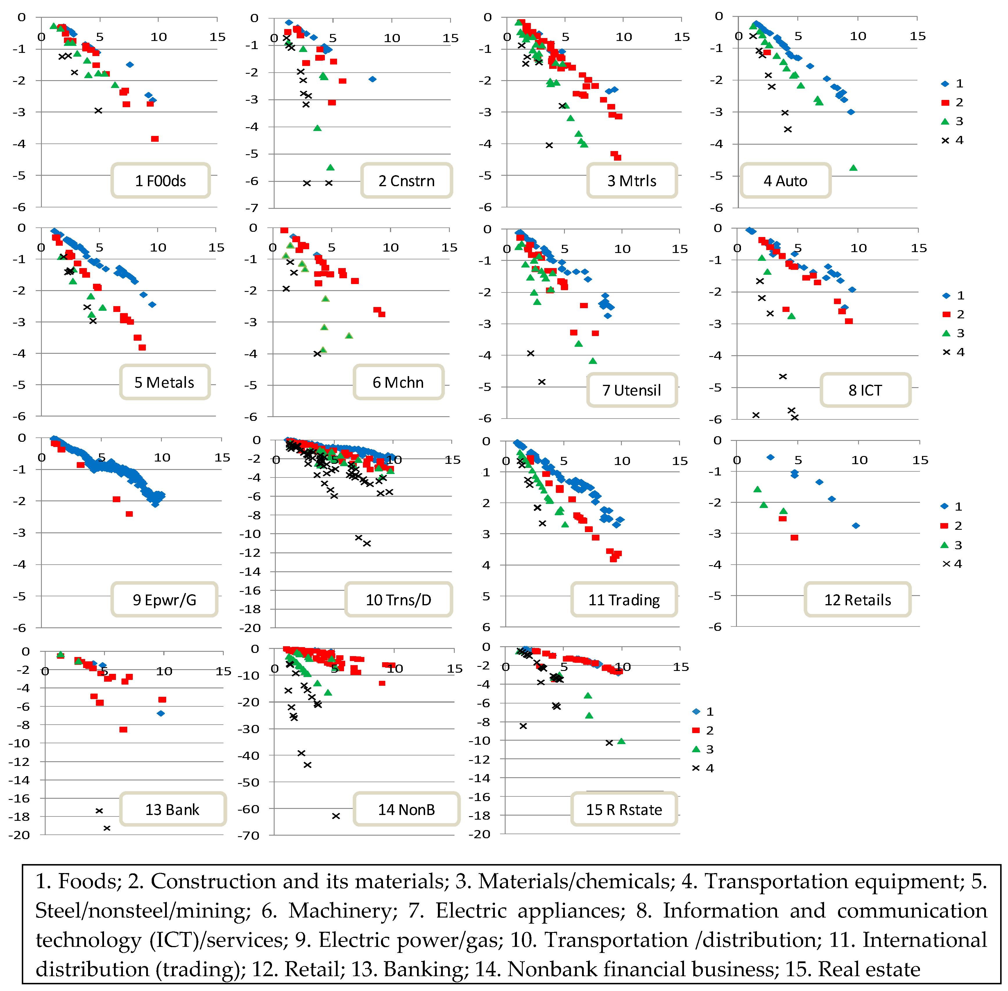
3. Crisk Analysis of R&I Credit Ratings via CRiPS Measures

Consequently, we call M3-CRiPS simply CRiPS and the plot of ( s k M ( k ) , y k ( 3 ) ) for some ks in the two-dimensional plane the CRiPS-plot, where y k ( 3 ) is henceforth denoted by y k . In this section, the CRiPS structure of 1545 Japanese CBs as of August 2010 is analyzed in association with classification schemes such as the agency’s credit rating grouping and the industry grouping, and the Crisk homogeneity of these categorical groups is investigated by CRiPS-plots. The groups formed by the R&I credit rating, which is the rating of issuers, are shown to be inhomogeneous in Crisk quality and mostly not comparable beyond industry categories.
It is remarked that credit or industry categories or other categories, if any, are descriptive by nature and, strictly speaking, no categories can define the probabilistic populations under which CB prices are generated. This is because credit quality depends on many continuous factors, as discussed in Section 1, and because agency ratings are judgmental opinions based on broad viewpoints taking into account various factors. Hence, categorical credit ratings such as agency ratings are not the same as those of our Crisk rating based on default probability.
That said, let us consider whether the credit rating groups of the R&I are effective as Crisk-homogeneous groups over all the CRiPSs. The R&I credit rating is the credit rating of issuers as the CB stands, hence it may be not appropriate for CBs of various maturities because their time horizons are not explicitly taken into account in the rating, though it is often used in Japan. Table 2. gives the distribution of CBs in the R&I ratings of issuers as of August 2010.
Here, since some CBs issued by firms can belong to the same credit category, the CBs rated AA+, many of which are issued by 11 electric power companies, dominate the other categories in terms of number of CBs.
The first row of the table denotes the credit rating categories of R&I, the second row the number of CBs in each category, and the third row their proportions relative to the total 1454, where NA denotes no ratings. About 800 CBs are rated at least AA−.
To see whether these R&I ratings are consistent with our CRiPS measures, for simplicity the above 11 rating categories are integrated into four groups:
(1) G1: AAA, AA+, AA, AA−,  (2) G2: A+, A,
(3) G3: A−,(4) G4: BBB+, BBB, BBB−, C+.
Based on this grouping, we constructed a CRiPS-plot for each group, shown in Figure 5.
This figure shows that the CRiPSs of groups 3 (▲) and 4 (×) are spread over the plane and mixed into the regions of those of groups 1 (◆) and 2 (■). Hence the groups obtained by the R&I credit rating cannot be regarded as Crisk-homogeneous in terms of CRiPS measure. This will be confirmed in the next section, where a cross-table of all R&I rating groups and the Crisk-rating classes to be defined are given.
Consequently, as seen in Figure 5, the R&I credit rating category alone is not good at getting Crisk-homogeneous groups to derive TSDPs when all CRiPS measures are treated simultaneously. In our Crisk rating, from a practical and forward-looking standpoint, we stick to the CRiPS measures realized in the market and will form Crisk-homogeneous groups by our Crisk rating system.
Next, we combine the R&I credit ratings with the industry groupings. In Figure 6, industry-wise CRiPS-plots are made with the above groupings of R&I credit ratings distinguished. Looking at the shapes of these graphs, we find a strong linear structure of CRiPSs in maturity at least for each group in each industry, though the linearity is not well shown for some industries. This result shows that the cross-category of R&I rating and industry classification will conform to the linearity of our CRiPS measures, so may imply that the R&I uses the industry category in the rating. This, and some other observations lead us to the definition of the standardized CRiPS in the next section.
Among the industry categories, electric power, international distribution (trading), and metal are more closely investigated below.

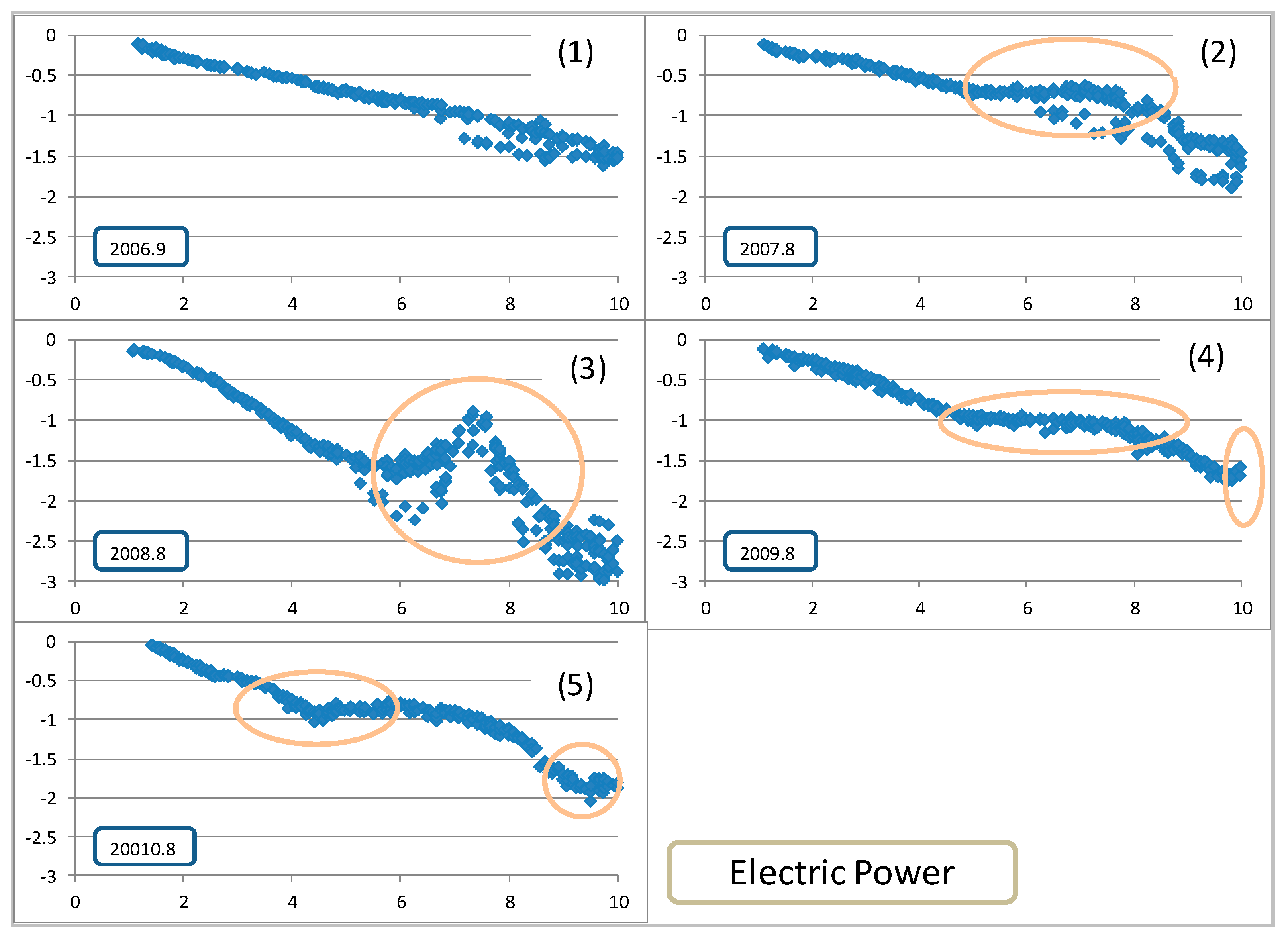
3.1. Electric Power Industry

In the case of the electric power industry, there are 10 monopolistic regional companies and one special company (J-Power), and they issue about one-third of Japanese CBs, whose R&I credit ratings are all in G1 (◆). This is because those companies are regarded as being backed up by the government. In graph 5 of Figure 7 for the CB data of August 2010, there are some kinks near 5 years, 7.5 years, and 9 years, so they are not in a strong linear relationship with y k and s k M ( k ) . To find a reason for this, the time series changes of the CRiPS-plots are given in Figure 7 for the following time points: (1) August 2006, (2) August 2007, (3) August 2008, (4) August 2009, and (5) August 2010.
Some interesting observations can be made from Figure 7:
(1)
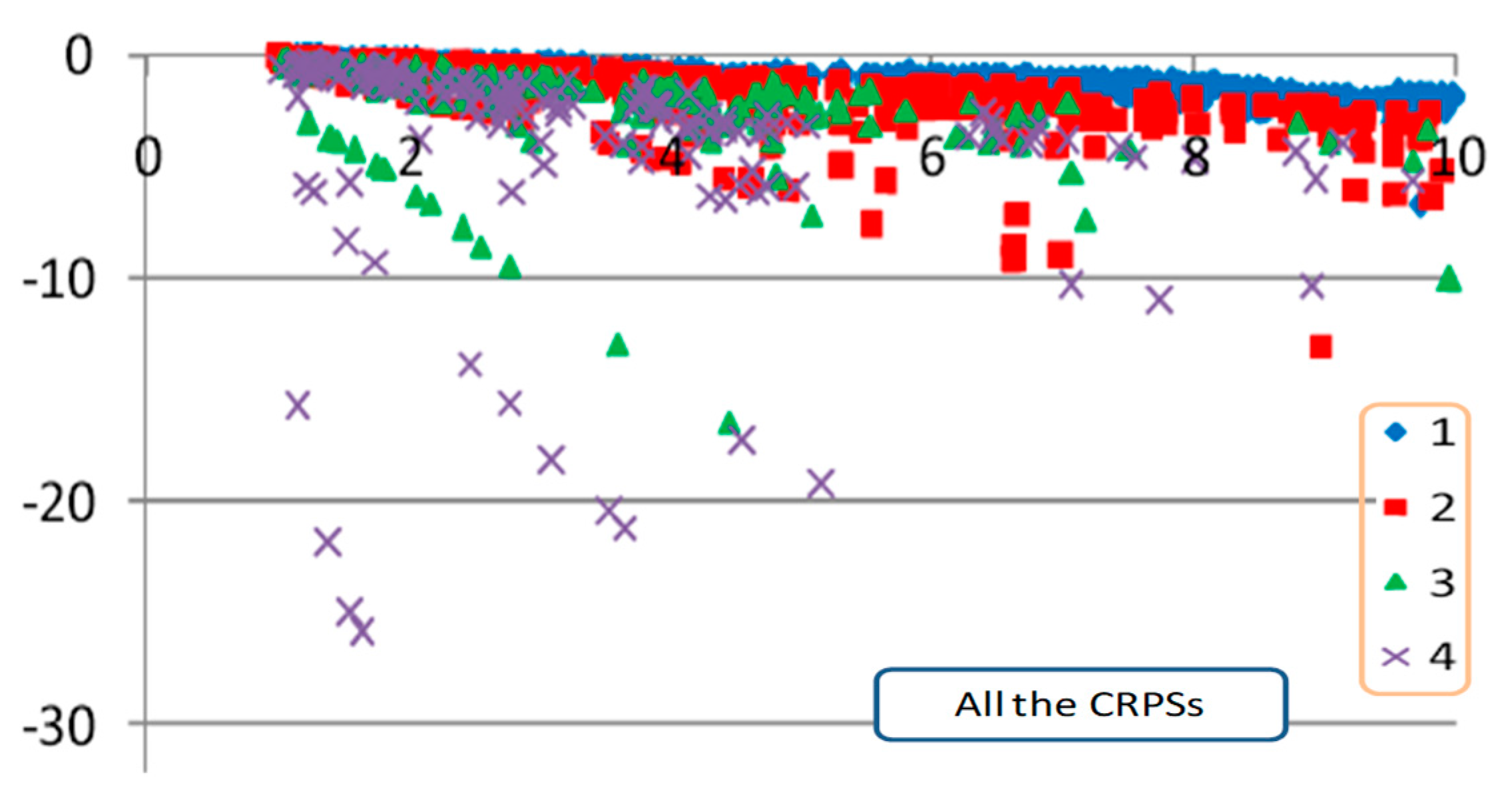
In graph 1, in September 2006, in the middle of the growing economy, the CRiPSs of the CBs were almost perfectly on a straight line, and the term of 10 years y k attains the largest (best) value of −1.6 yen among the five cases (graphs), which is larger (better) than August 2010 in graph 5. Around the term of 7 through 10 years, the two divided lines in graph 1 are confirmed to correspond to the Crisk preferences of some issuers for CBs in the electric power industry. The differences of the market Crisk preferences for some specific issuers in August 2010 are identified in terms of TSDPs in Section 5.
(2)
In August 2007, when the economy was around the peak of the business cycle, investors who expected a coming downturn of the economy deformed the pattern of the CRiPSs with stronger Crisk preferences and some maturity preferences appearing around the 7-year term (see graph 2). In fact, around the terms of 5–7 years, the CRiPSs in the upper line in graph 2, about −0.7 yen, were better than in graph 1, implying that more of those CBs were bought. In addition, the Crisk preference became stronger for terms of 6–10 years.
(3)
The maturity preference continued until the financial crisis period in graph 3. CBs of about 7-year maturity were strongly preferred, though the level of the CRiPS was lower (worse) than in graph 2. What is notable here is that the CRiPSs around 10 years are large enough in absolute value to be close to −3 yen, which is significant relative to those of graphs 1 and 2. The gap between the 7-year and 10-year CRiPSs is as big as 2 yen. This implies that the linearity observed in graph 1 was disturbed by a big crisis.
(4)
In graph 4, one year later, the CRiPSs returned to the same shape as in graph 2, though the level is a bit lower (worse), and no issuer preference is observed here.
(5)
Under the continuation of bad economies in Japan and world, some maturity preferences seem to appear in graph 5, though no issuer preference can be seen.

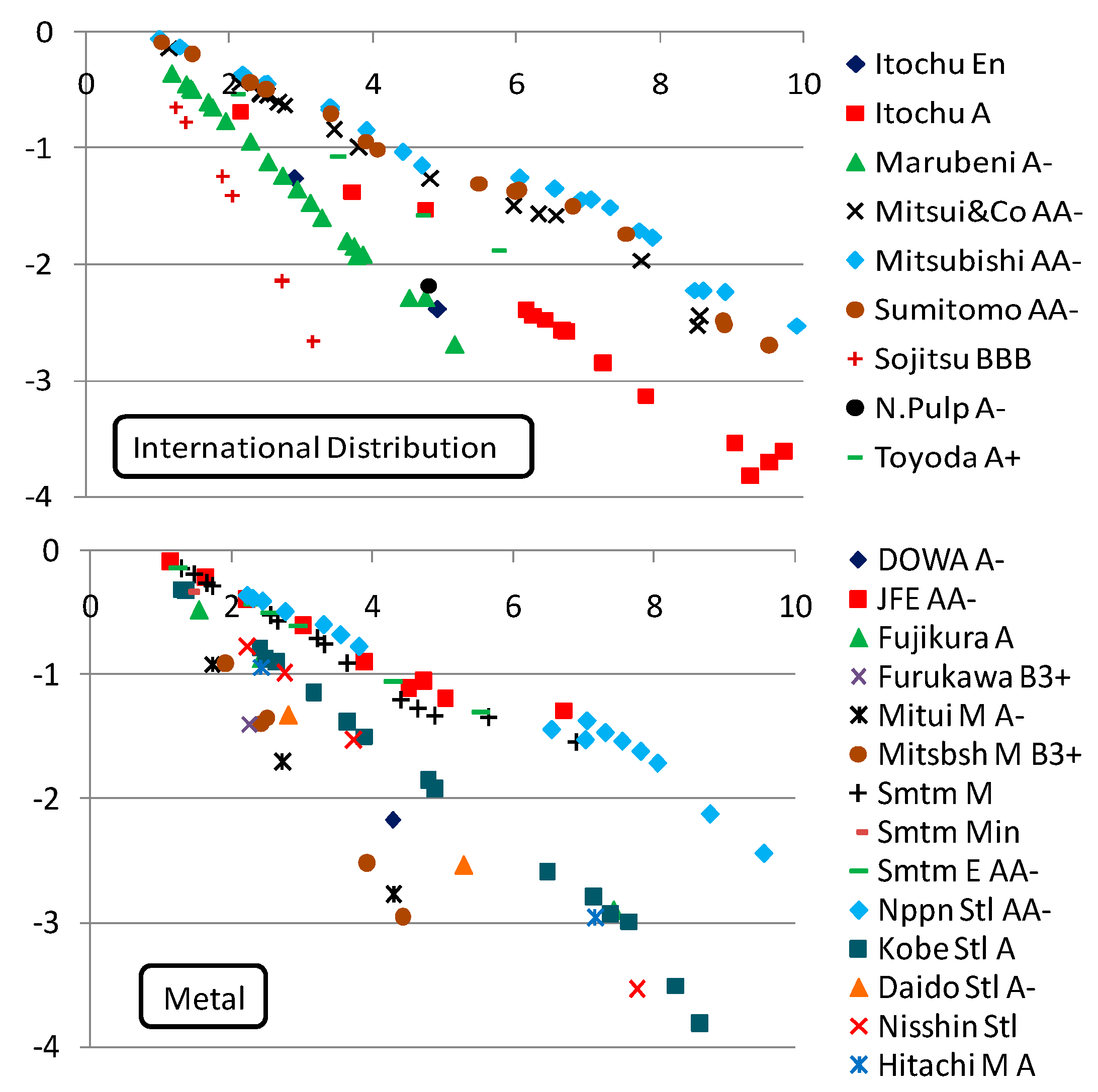
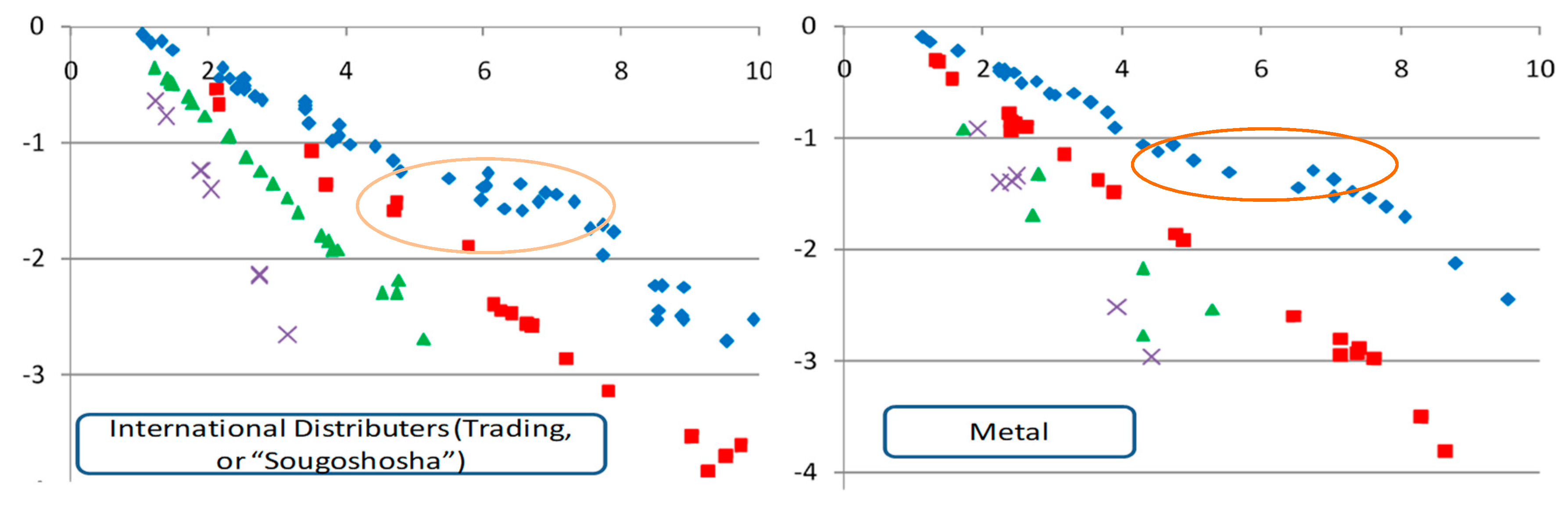
3.2. Trading and Metal Industries

Graph 1 of Figure 8 shows the CRiPS-plot for the CBs in international distribution (or simply trading). In the trading industry, the R&I credit ratings distinguish four groups, while in steel and nonsteel/mining (or simply metal), G3 (▲) and G4 (×) are not well distinguished. Note that G1 (◆) of CRiPSs in the trading industry is almost uniformly smaller (worse) than that in electric power,
which also shows the noncomparability of the R&I ratings beyond the industry category. In these industries, the graphs of G1 CRiPSs show some kinks corresponding to the electric power industry, while the CRiPSs of G2–G4 are almost linear in maturity. This implies that the market sensitivity of CB investors to shock in G1 is greater.
The enterprise-wise Crisk structure of these industries is described in Figure 9, together with R&I ratings. The graphs show a strong linear structure of enterprise-wise CRiPSs in maturity, except for some high-quality CBs with some flat areas in the middle terms. This shows the effectiveness of the CRiPS as a measure that can distinguish the enterprise-wise credit quality rather linearly.
In Section 5, enterprise-wise TSDPs of some firms in these industries will be derived in the case where relatively many CBs exist. In particular, time series movements of TSDPs are investigated for TEPCO and Mitsubishi Corp.

4. Crisk-Homogeneous Grouping by Cluster Analysis and FIS via S-CRiPS Measure

In this section, to make Crisk-homogeneous groups, we use two empirical grouping methods:
(1)
Three-stage centroid clustering, and
(2)
fixed interval filtering with x-yen split rule.
Here, the CRiPS measures { y k } of CBs with different maturities { s k M ( k ) } issued by a firm tend to be linear in maturity, implemented by defining the standardized measure of the CRiPS:
ς k = y k / s k M ( k ) ,
which we call the S-CRiPS measure or simply S-CRiPS.
(1)
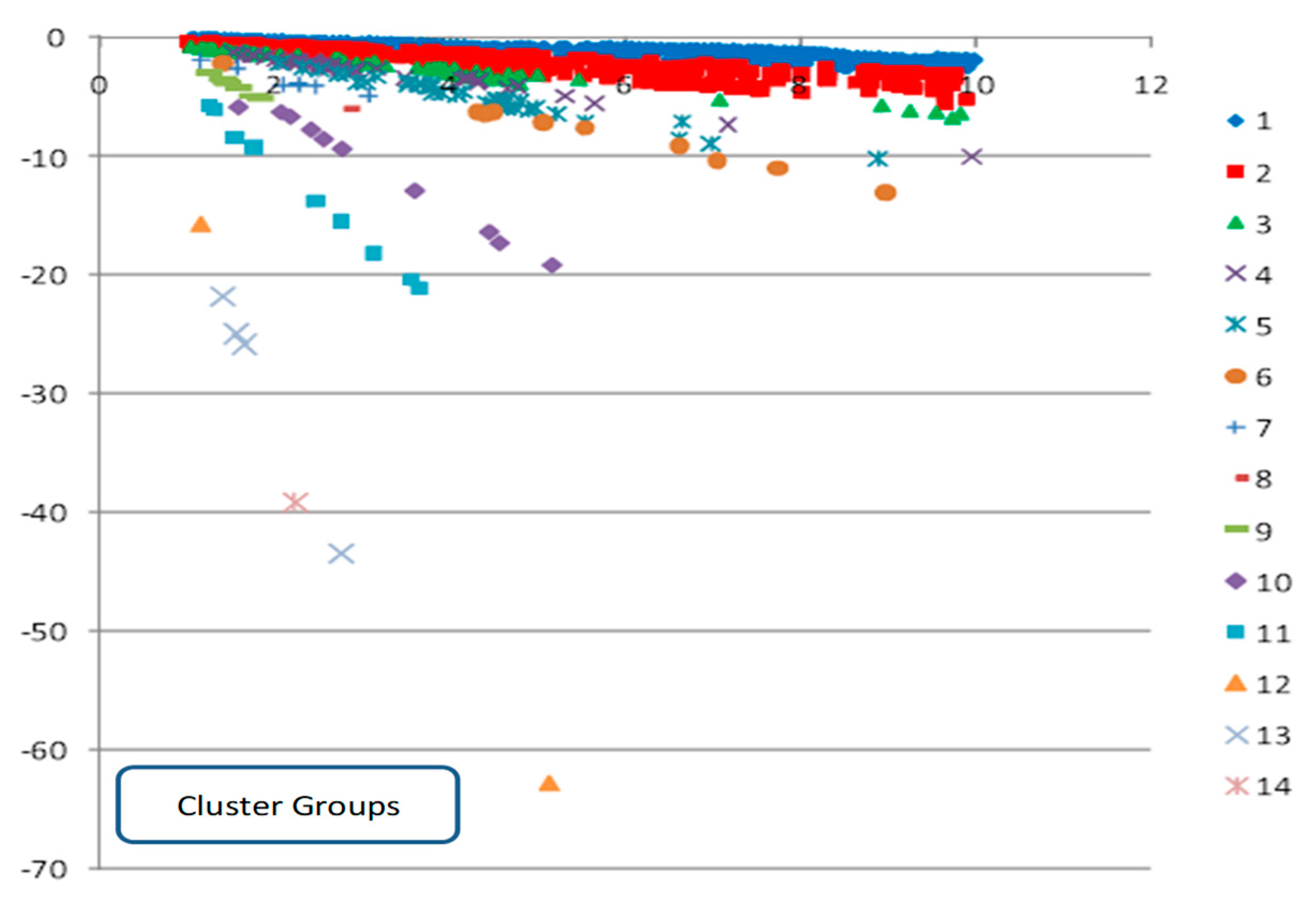
First, we apply a three-stage centroid cluster method to the S-CRiPSs to get 14 Crisk-homogeneous cluster groups (CGs). The first cluster group (CG1) of the CBs that are closest together in the S-CRiPS is found to be the largest group in terms of number of CBs, implying that even three-stage centroid clustering does not sufficiently classify CBs because of the mutual closeness of too many S-CRiPSs.
(1)
Alternatively, as an absolute criterion for grouping and rating CBs, we propose the Crisk rating system with a set of fixed intervals filtering Crisks in terms of 10 times S-CRiPS, i.e., 10 ς k , where each 10 × S-CRiPS of a CB is assigned to a rating interval in the half line (−∞,0]. It is noted that by the definition of Equation (13), 10 ς k is 10-year-maturity-equivalent CRiPS measure of y k and the straight line connecting (0,0) and ( s k M ( k ) , y k ) passes (10, 10 ς k ). The choice of a set of fixed intervals is made by dividing the half line (−∞,0] by an x-yen split, where x-yen is the basic unit of making intervals for 10 ς k s. For Japanese CBs, x = 1 is proposed (below), except for large S-CRiPSs in absolute value, and each CB is empirically rated by the number of fixed intervals. The market price–based categorical rates thus made can be used for investment decision-making and credit portfolio analysis in asset management, since the ratings are universally comparable over all CBs.

4.1. Crisk-Homogenous Groups via Cluster Analysis

Here, the three-stage centroid cluster method is applied to all the S-CRiPSs {10 ς k } to get empirically Crisk-homogeneous groups, where the centroid distance is defined as the Euclidean distance. In the analysis, the number of clusters to be made is fixed in advance at six clusters for each stage, and finally 14 credit homogeneous groups are formed. Since 10 ς k is univariate, cluster grouping is nothing more than forming groups by ordering the measures in the half interval (−∞, 0] and making appropriate sub-intervals for CBs to be put into. The procedure is as follows:
(1)
All 1545 CBs, including subordinated bonds, are clustered into six groups. The result is given in the upper part of Table 3. Clusters 3, 4, 5, and 6, which are very far away from 1 and 2 in centroid distance (13.86 − 4.67 = 9.19), are recognized as independent clusters and named CG11, CG12, CG13, and CG14. These clusters do not include many CBs; CG11 consists of CBs issued by Promise (BBB+, nonbank) and Daikyo (BBB, real estate), and CG12–CG14 consist of CBs issued by Aiful (CCC+, nonbank) only. Hence, it is difficult to derive the TSDPs for these groups due to a lack of samples. The members of these clusters are excluded in the second stage cluster analysis.
(2)
The 1529 remaining CBs, whose CRiPS measures are greater than −4 yen, are again clustered into six groups, and the middle part of Table 3 gives the result. Here again, clusters 3, 4, 5, and 6 are separated from 1 and 2, and form independent clusters CG7, CG8, CG9, and CG10. The centroid distance between clusters 1 and 2 and clusters 3–6 is still as large as 1.83 − 1.03 = 0.80 (yen).
(3)
The remaining 1505 CBs, whose CRiPS measures are greater than −1.5, are then clustered into six groups. Though these are relatively indistinguishable, we call them CG1 through CG6 in order of Crisk quality. CG1 still contains 988 CBs. The centroid distance between groups 1 and 2 and 3–6 is as small as 0.458 − 0.317 = 0.141. We stop here, because a further breakdown would not yield meaningfully distinguishable groups.
The cluster groups are summarized in Table 3. It is clear from this table that CGs 12, 13, and 14 are exceptionally distant from the other clusters and only contain small numbers of CBs. The table shows that CG1 and CG2 contain 988 and 351 CBs, respectively, more than the other clusters. This implies that the cluster analysis as it stands may not provide significantly distinguishable groups.
Now, based on this cluster grouping, the CRiPS-plot is again made for all CBs in Figure 10, where the 14 CGs are distinguished by symbols. The graph shows that the 14 CGs are appropriately and linearly separated.
CG1 and CG2 are analyzed in terms of industry category. In Table 4, the CBs in CG1 and CG2 are decomposed into our 15 industry categories, though how to classify industries is a different important issue. Besides, it is quite common in our global era for each firm to have some business lines that belong to different industries, whatever the industry classification may be. Typically, the stock exchange authoritatively assigns each firm to an industry category when it is listed. Hence, the concept of industry categories itself is a practical concept for convenience.
From Table 4 it is observed that the CBs in specific industries such as 9 and 10 belong to CG1 more than those in other industries. The distribution is structured this way because some firms with high credit quality simply issue more CBs, as has been observed in the electric power industry. In fact, a large portion of capital in the market is invested in the electric power industry, which in turn suggests high liquidity of the market as well, because these CBs are regarded as “safe” by investors.
One of the problems with forming groups by cluster analysis is that since the CRiPS measures are stochastically realized, the points splitting CBs to form clusters in the half line (−∞,0] move around stochastically. Hence, the ratings made by the cluster grouping are dependent on the economic environment.
In the next section, the TSDPs are derived for groups G1 through G7, with the industry classification for G1 and the default risk structures compared in terms of default probabilities; groups CG8 through CG14 are ignored in in this derivation because of the small samples.

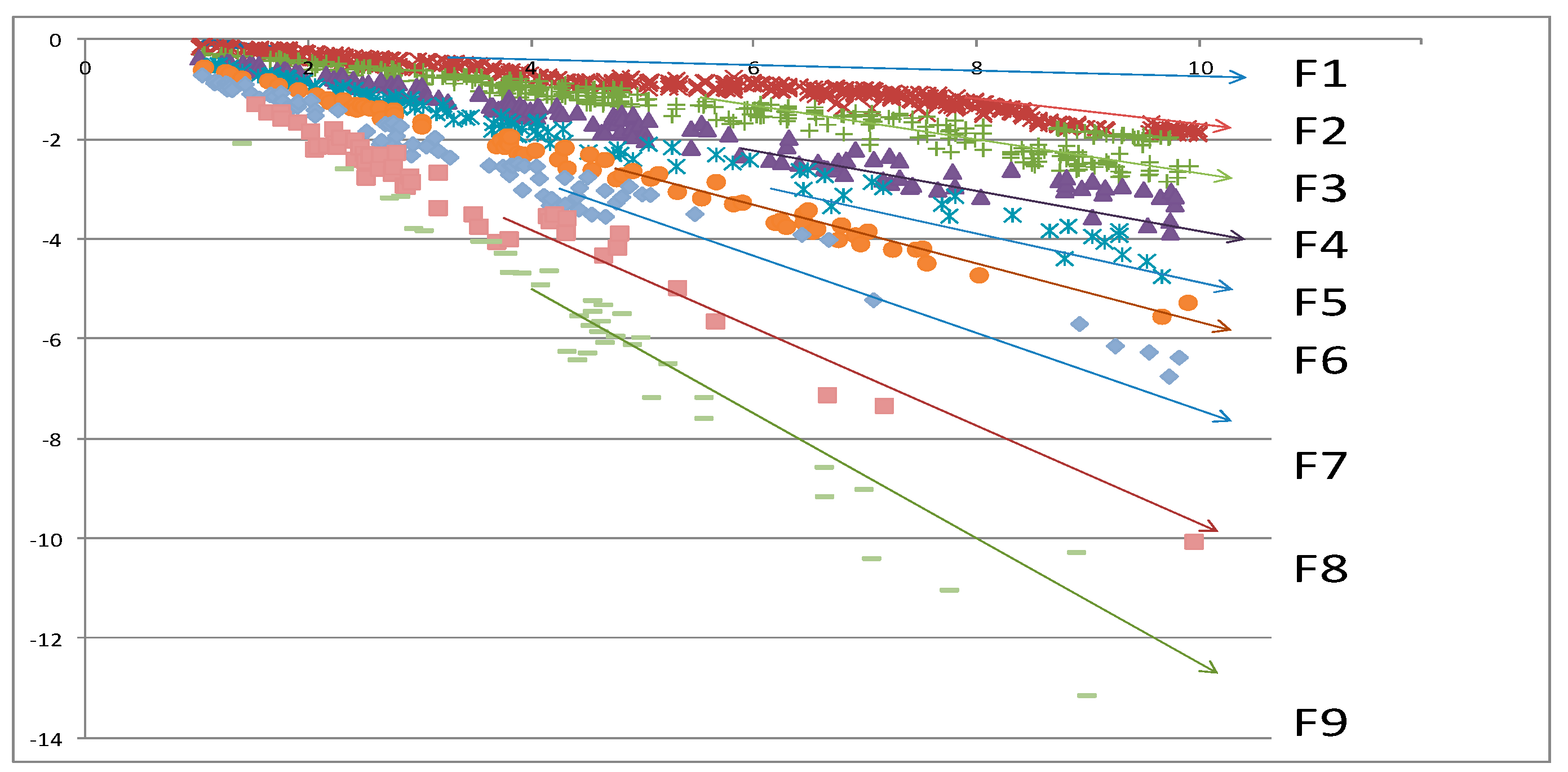
4.2. Crisk-Rating System with Fixed Interval Scheme for S-CRiPSs

It will be useful to have a fixed criterion for credit ratings independent of the economic environment to give us a measure that guarantees a certain level of default probability (DP) for decision-making in investment and risk management. For such a measure, we propose a fixed interval scheme (FIS) with 1-yen rule that gives Crisk-homogeneous classes. Once it is accepted, we can rate the credit risk of a CB at any time by the Crisk class it belongs to and discuss the transitions of the ratings over, e.g., monthly periods by a transition matrix method. This approach is an agency rating–free and forward-looking market approach to see the changes of investors’ views in the markets.

4.3. Comparison of Our Crisk Rating and R&I Rating

Next, the FIS-3 that we propose is made to relate to the R&I agency credit ratings. Let the 10 classes formed by FIS-3 be denoted by F1 through F10, which are regarded as Crisk rating groups.
Now, to get such a FIS, first let us consider the distributions of the 10 ς k s in the half line (−∞,0] with different split units.
In Table 5, five promising FISs are considered for our Crisk-rating system, where the Crisk-homogeneous classes they provide are called F classes.
FIS-1 of Table 5 is the case with x = 0.5. The distribution with 0.5 yen split unit applied up to −6 yen and 1 yen split unit thereafter explicitly shows the credit structure of CBs in terms of 10 ς k . It has a mode in the interval [−2.0,−1.5) in F4 and a gradually decreasing tail toward −8 yen. Beyond −8 yen, 10 ς k s are scattered far away toward −∞. On the other hand, in FIS-1 the first and second groups may be too refined, and taking into account the stochastic nature of 10 ς k , the distributional information will be too detailed with too many groups generated.
The distribution of FIS-2 with 1 yen split unit up to 10 yen and the rest combined into one seems to provide more appropriate groups for ratings. Compared to FIS-1, the mode moves from F4 to F2, and F1 and F3 in FIS-2 become larger around the mode and F4, F5, and F6 become smaller. FIS-3 is the modified version of FIS-2, combining some tail parts beyond −6 yen. We propose this FIS, as the division rule of the half line though the number of CBs in F6 of 1 yen split is smaller than that of CBs in F7 of 2 yen split. The distributions of FIS-4 and FIS-5 with split units of 1.5 yen and 2 yen, respectively, are described in Table 5. Clearly the groups formed by the rules are much less informative about the Crisk structure.
We call the credit rating system with FIS-3 the Crisk-rating system, with 10 Crisk- homogeneous classes (or simply Crisk classes).
In Table 6, each row shows the distribution of CBs in each R&I rating category over the Crisk rating classes F1–F10. It is observed that most CBs with AAA, AA+, AA, and AA− ratings belong to F2 and F3, so they are relatively difficult to be distinguished in the 10ζk measure. The CBs in R&I rating categories of A+, A, and A− are more broadly scattered over FIS classes. Except for AAA, the modes of all R&I rating distributions over FIS classes are consistent with the order of the Crisk rating classification if the equality is included. However, although the mode of AA belongs to F2, for example, 45% of the 119 CBs with AA rating are assigned to F3, while 27.9 % of CBs with AA− rating are assigned to F2, although the mode belongs to F3.
On the whole, the lower the R&I rating, the more the distribution deviates from the mode up to that of BBB. This implies that the lower the rate, the less stable the Crisk quality in our measure and the less liquidity.
Using our Crisk rating classification, the CRiPS-plot is made in Figure 11. The groups are well separated as Crisk-homogeneous classes by way of our rule.

5. TSDPs for Individual Firms, Cluster Groups with Industry Categories, and Crisk-Rating Classes

Via Kariya’s (2013) model, we derive the TSDPs of cluster groups, CBs of some firms in industries treated in Section 3, and the Crisk-homogeneous classes or equivalent Crisk-rating classes in Section 4. Note that the TSDP of each Crisk class is nothing but the forward-looking common views on DPs shared by CB and GB investors.
Consequently, the following TSDPs are derived:
(1)
For some individual firms in the electric power, international distribution (trading), and metal industries, where the firms issue relatively many CBs
(2)
For the top seven cluster groups identified above (CG1–CG7)
(3)
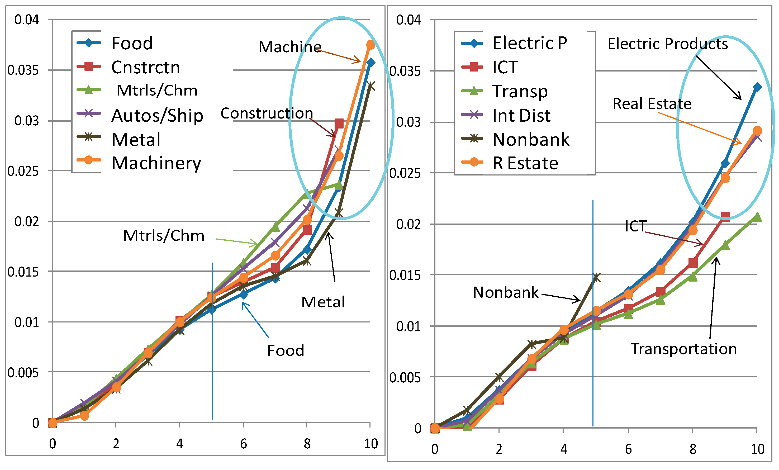
For industry groups CG1(1), CG1(2), …, CG1(14) obtained by decomposing CG1
(4)
For Crisk-rating classes F1, F2, …, F7
In particular, the time series movement of TSDPs of TEPCO is described over the period September 2006 to August 2010.

5.1. Model for Pricing CBs and Deriving TSDPs

To claim the effectiveness of our empirical results in this section, we review our model from Kariya (2013) that includes the TSDP of each CB in pricing. As in the case of GB in Section 2, let the kth CB price model for { V k } be
V k = j = 1 M ( k ) C ¯ k ( s k j ) D k ( s k j ) ,
where D k ( s k j ) is an attribute-dependent stochastic discount function and s k j is the time at which the jth CF is generated. Then by Equation (5) the model is expressed as
V k = j = 1 M ( k ) C ¯ k ( s k j ) D ¯ k ( s k j ) + ε k   w i t h   ε k = j = 1 M ( k ) C _ k ( s k j ) Δ k ( s k j ) .
The main feature differentiating this model from the GB model in Equation (6) is the CF function C ¯ k ( s k j ) , because the scheduled CFs are not guaranteed when the issuer of the CB defaults. The TSDP of the kth CB is given by the accumulated default probability function p k ( s ) with 0 < s s k M ( k ) . Here, as the expectations of investors, the CF at s k j is specified as
C ¯ k ( s k j ) = C k ( s k j ) [ 1 p k ( s k j ) ] + 100 γ [ p k ( s k j ) p k ( s k j 1 ) ] ,
where p k ( s k j ) = P ( τ k s k j ) is the (accumulated) default probability up to time s k j with τ k default time, and γ is a recovery rate when the issuer defaults. The first term of the right side is coupon times nondefault probability and the second term is the CF when the issuer defaults in the period ( s k j 1 , s k j ], which is principal 100 times γ times the default probability in that period.
Unless the issuer issues sufficiently many CBs with different maturities, we cannot estimate this individual TSDP of the issuer. In this case, a Crisk-rating class is used to estimate a common TSDP for each class, where the recovery rate is assumed to be common. Then let p ( s ) be a common TSDP where p k ( s ) = p ( s ) and let it be approximated uniformly by a polynomial of order q:
p ( s ) = α 1 s + α 2 s 2 + + α q s q ,
where in our analysis we assume q = 5. Then, inserting Equations (16) and (17) into Equation (15) yields
y = X ( γ ) β + ε   w i t h   X ( γ ) = X 1 + γ X 2 ,
where β = ( α 1 , , α q ) and the kth element of explained vector y ˜ is the kth CRiPS measure (see Kariya (2013) for details):
y k = V k P ^ k ,    w i t h    P ^ k = j = 1 M ( k ) C k ( s k j ) D ¯ k ( s k j ) .
Here, as has been discussed when the CRiPS measure is defined, our choice of P ^ k is
P ^ k ( 3 ) = j = 1 M ( k ) C k ( s k j ) D ¯ k ( 3 ) ( s k j )
where the attribute-dependent mean discount function D ¯ k ( 3 ) ( s ) is estimated by the GB prices at the same time and is simply denoted by D ¯ k ( s ) . In Equation (18) the regression matrix involves unknown recovery rate γ , which can be estimated under certain conditions (see Kariya 2013). The covariance structure is similar to the GB case, though it contains β (shown in Appendix A).
Consequently we assume γ = 0, because the recovery rate for each firm is not only different but also very uncertain in value at time 0. In addition, the time for creditors and stockholders to obtain their portions is also very uncertain. In fact, it depends on the bankruptcy law, such as Chapter 7 (liquidation) or Chapter 11 (reorganization) or other laws, as in the case of US Bankruptcy Law. It often takes one year or more to get the approval of creditors and the court. In the case of reorganization, creditors are often paid some portion of credits after a few years from the time of default. In this sense, it is not sensible to commit our research to this problem. In addition, setting γ = 0 leads us to a common base to evaluate and compare TSDPs among different firms and groups.

5.2. TSDPs of Individual Firms and Credit-Homogeneous Groups

The above model is applied to derive TSDPs with γ = 0. Our data consist of the set of CB and GB prices as of August 2010, and we use only CB prices whose maturities are more than 1 year and less than 10 years because of marketability of CBs. Further, TSDPs are graphed up to the time horizon of the maximum maturity of CBs in each group.

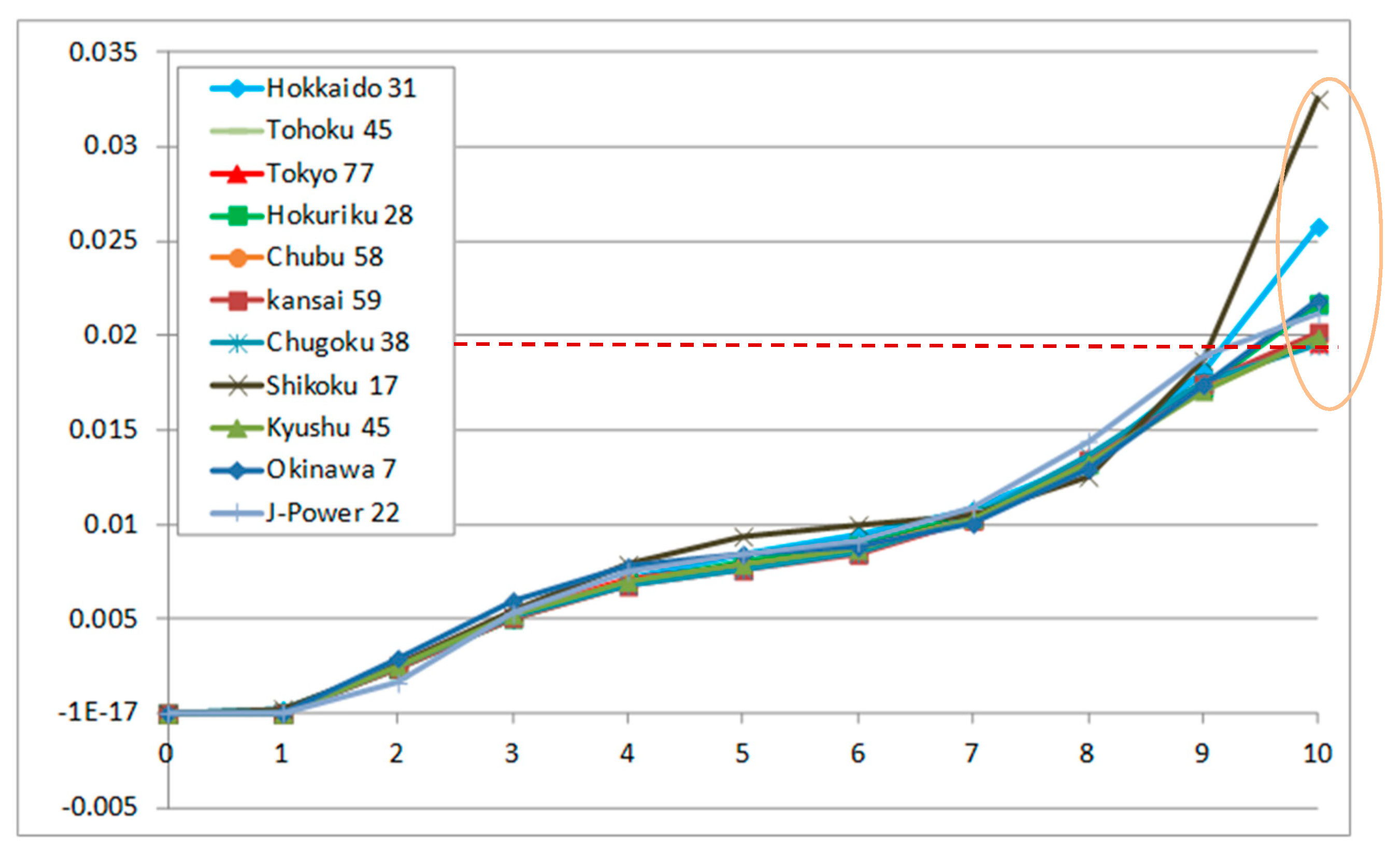
5.2.1. TSDPs of Individual Firms in the Electric Power Industry

First consider the electric power industry, whose CBs all belong to CG1. The industry consists of 11 companies (numbers in parenthesis are CBs issued): Hokkaido (HKD) (31), Tohoku (THK) (45), Tokyo (TKY; TEPCO) (77), Hokuriku (HRK) (28), Chube (CHB) (58), Kansai (KNS) (59), Chugoku (CGK) (38), Shikoku (SKK) (19), Kyushu (KYS) (45), Okinawa (OKW) (7), and J-Power (J-P) (22). Except for Okinawa, there are enough samples to estimate individual TSDPs, since the model includes seven parameters at most. Below, we also estimate the TSDP of Okinawa.
The TSDPs in Figure 12 are almost indistinguishable up to the time horizon of 9 years, with DPs of about 1.8%. The accumulated DPs are commonly 2.0% in 10 years, except for Hokkaido and Shikoku Power, whose DPs are respectively 2.6% and 3.3% in 10 years. The DPs of Okinawa Power are slightly higher than those of companies in 2–3 years and 10 years, and of Hokkaido Power in 4–7 years, implying that these companies are rated slightly lower in credit quality. The default probabilities at 10 years are rather separated among the 11 companies, and those of Shikoku, Hokkaido, and Okinawa are higher than the others. The TSDP of Tokyo is found to be uniformly smaller than the others.

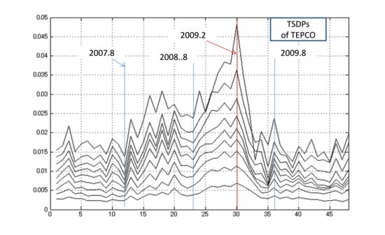
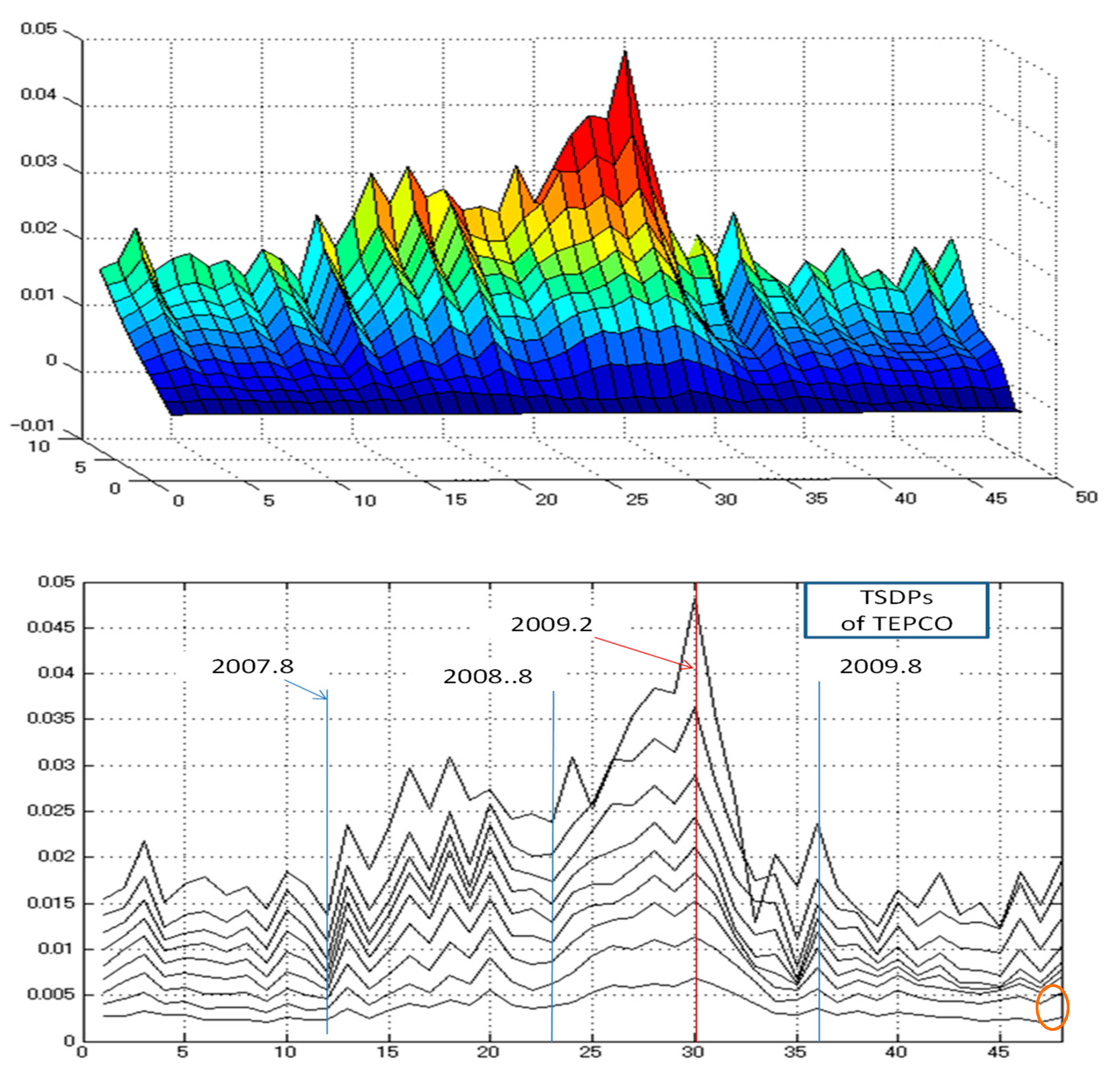
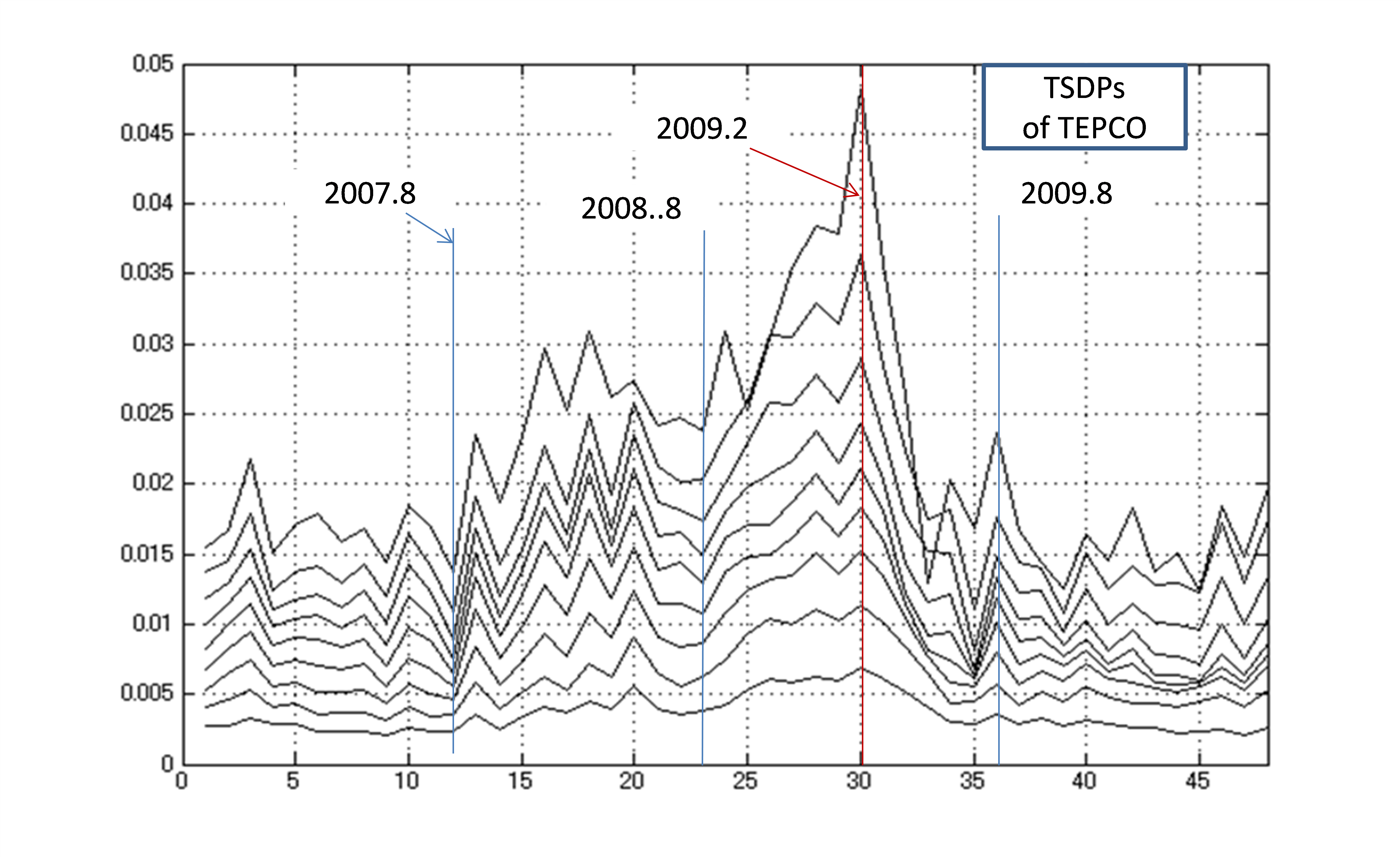
Monthly Changes of TSDPs of TEPCO from September 2006 through August 2010

In Figure 7, it was observed that the term structures of CRiPSs { y k } in the electric power industry in September 2006 were almost perfectly linear with respect to maturity { s k M ( k ) } and changed their pattern along business cycles. Here, to look at the time series movements in terms of TSDP, taking TEPCO as a representative firm, we derive its monthly time series TSDPs over the period September 2006 through August 2010, where the sample size of each month is at least 60 and at most 80.
Both graphs in Figure 13 give the time series movements of TEPCO’s TSDPs. The upper graph describes 3D movements of the TSDPs, while the lower one represents the time series variations of DPs { p t ( s ) : t = 1 , 2 , , 48 } for each s = 2, …, 10.
(1)
In the time series of 10-year DPs, the maximum DP is 4.8% in February 2009, which is due to the financial crisis that started in September 2008. It is interesting to note that the JGB market was affected the worst in November 2008, though the reason for the time lag of TEPCO’s CBs is not clear.
(2)
The period of the first 12 months from September 2006 was in the upturn economy during which TEPCO enjoyed high revenues, and hence the TSDPs are overall lower, with 10-year DPs of about 1.6%. The curves of the TSDPs are not steep.
(3)
In the second 12 months starting from September 2007, the TSDPs rose rapidly and the 10-year DP attained 3% in February 2008, when the economy went down.
(4)
In September 2008 during the Lehman shock, the 10-year DP was 2.6%, which is a bit amazing because our end-of-month CB price did not respond to the shock on the spot. However, the DPs then increased dramatically to 4.8% in February 2009, and thereafter decreased greatly within five months.
(5)
The period August 2009 through August 2010 is somewhat similar to the period in (1) except that the DP curves in this period have flat areas in the middle term, corresponding to Figure 7.
A careful investigation into such time series movements of the 10-year DPs will lead to a correspondence with business cycles or industry business cycles in macroeconomic analysis, though it is left over.

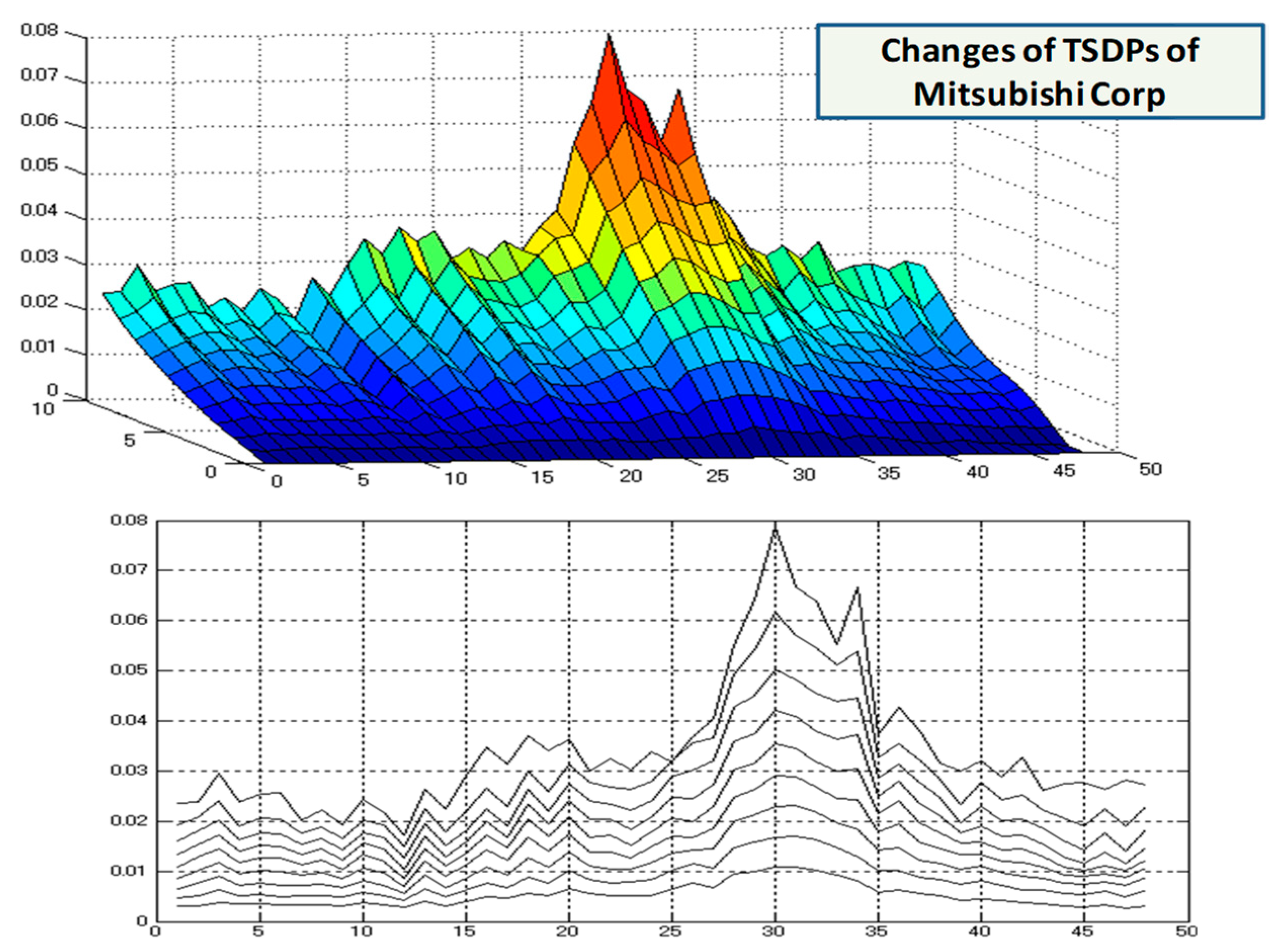
5.2.2. TSDPs of Individual Firms in International Distribution Industry

Second, let us consider the TSDPs of firms in the international distribution (trading) industry, for which the CRiPS structure of the industry and the firms are given in Figure 8 and Figure 9. In Figure 14, their TSDPs are graphed.
A uniform ordering of the TSDPs of the firms in this industry is exhibited, and the top four are Mitsubishi Corp., Sumitomo Corp., Mitsui & Co., and Itochu Corp., whose 9-year DPs are respectively 2.3%, 2.55%, 3.0%, and 3.7% and 10-year DPs in are respectively 2.7%, 3.1%, NA, and 3.8%; the first three firms have an AA− rating by R&I. These DPs are higher than those of the firms in the electric power industry. Obviously, Marubeni and Sojitz have much higher DPs, though the maturities of their CBs are less than 5 years.

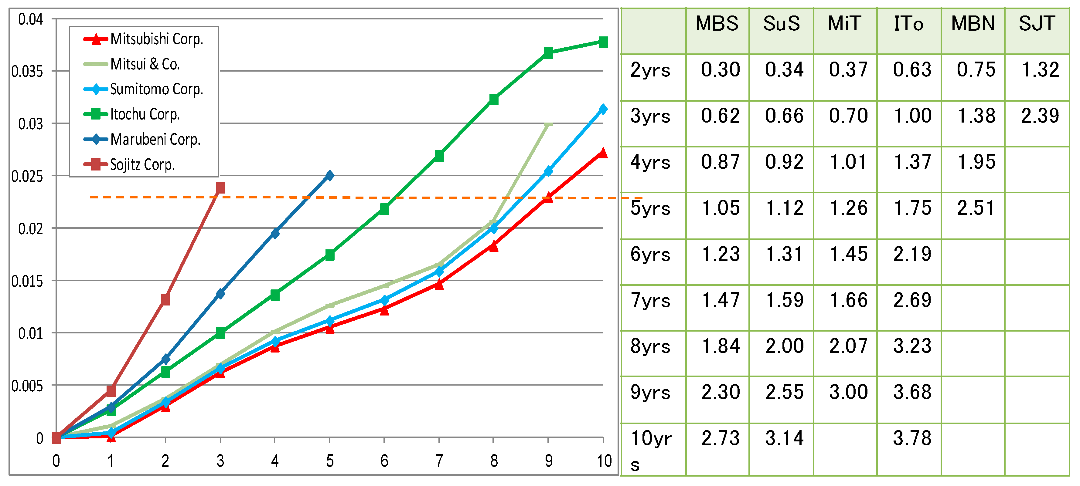
Monthly Changes of TSDPs of Mitsubishi Corp. for September 2006 through August 2010

For reference, the changes of the TSDPs of Mitsubishi Corp. are given in Figure 15. Clearly the worst TSDP took place in the 30th month, February 2009. A closer comparison shows that Mitsubishi’s TSDPs are uniformly larger than TEPCO’s for all time periods.

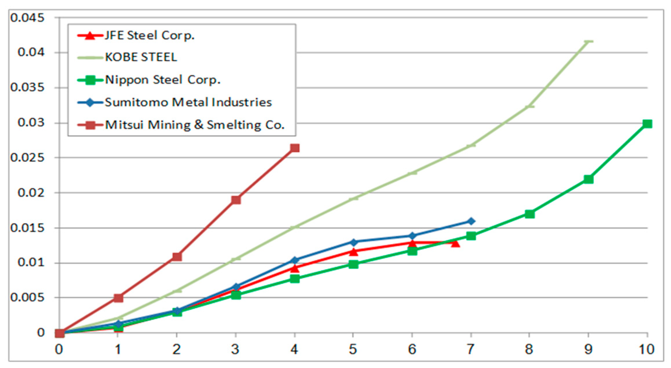
5.2.3. TSDPs of Individual Firms in Metal (Steel/Nonsteel/Mining) Industry

From Figure 16, similar observations can be made for the five companies in the metal industry. Clearly, Nippon Steel, JFE, Sumitomo, Kobe, and Mitsui Mining are distinctly ordered in the TSDPs, though the 7-year DP of JFE is a bit smaller than that of Nippon Steel, which is probably due to the lack of CB price data in the region for 5- to 7-year terms. Nippon Steel has an AA− rating by R&I and is almost uniformly better than the other companies in this industry. Its DP is rated as 3% in the 10-year term, which is larger than the DP of 2.7% of Mitsubishi Corp. with the same rating.

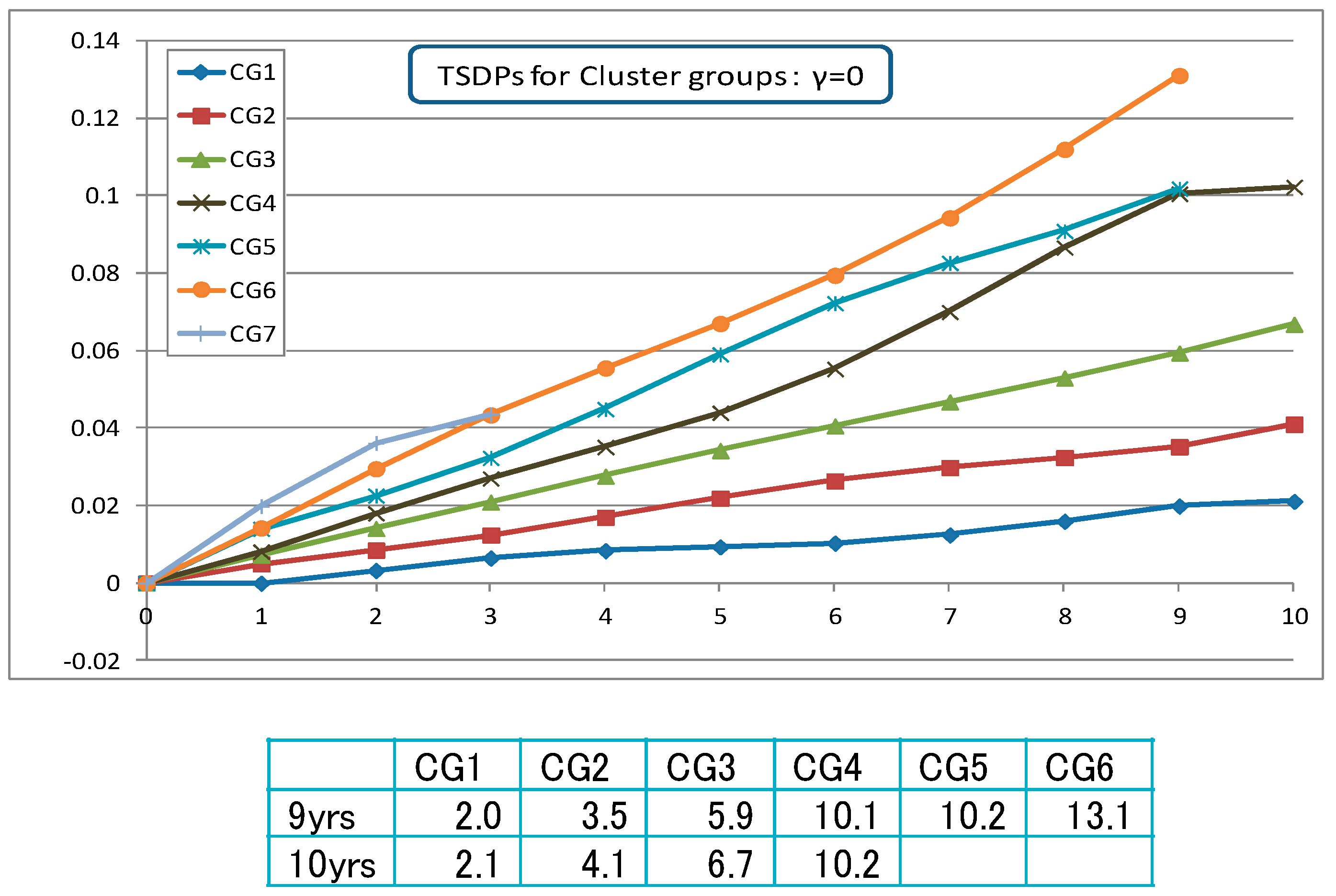
5.2.4. TSDPs of CG1–CG7

The TSDPs of the cluster groups are derived in Figure 17. They are well separated among the groups, as may be expected, by the method of cluster analysis, and the DPs of CG1–CG4 in the 10-year term are respectively 2.1%, 4.1%, 6.7%, and 10.2%. The differences of these DPs increase: 4.1 − 2.1 = 2.0, 6.7 − 4.1 = 2.6, and 10.2 − 6.7 = 3.5. Note that the numbers of CBs in CG1–CG4 are respectively 988, 351, 80, and 38, and CG1 and CG2 may have a different credit structure.
CG1, with 988 CBs, which is supposed to be Crisk-homogeneous as a whole, is decomposed into industry groups to see its diversification of industries.
In Figure 18 the TSDPs are drawn for the industry groups, and it is observed that in shorter terms the default probabilities are not much different among these industries, but in longer terms default probabilities are differentiated among industries; they are relatively larger in materials and chemicals and relatively small in metal (steel/nonsteel). In fact, at the 9-year term, DP is 3% in materials/chemicals, while it is 2.1% in metal and 1.75% in transportation (JR East Railway, etc.), so the differences are relatively large.

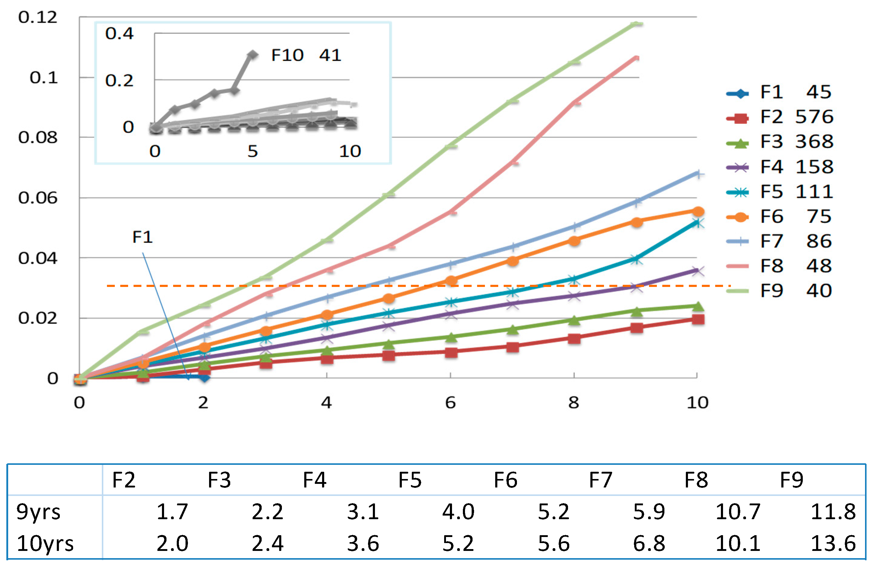
5.2.5. TSDPs of Crisk-Rating Classes

Finally, the TSDPs of the 10 Crisk-rating classes from Section 4 are similarly derived in Figure 19. The 10-year and 9-year DPs of F1–F9 Crisk-homogeneous classes are also listed, and the DP of F10 is 0.32 in the 5-year term, i.e., p F 10 ( 5 ) = 0.32 . Class F1 consists of 42 CBs whose maturities are less than 2 years and has DP p F 1 ( 2 ) = 0.00058 . These 42 CBs are regarded as almost perfectly default-free. The DP of F2 is p F 2 ( 10 ) = 0.02 , which corresponds to that of CG1.
As for applications of the TSDPs with Crisk rating classes, it will be interesting to see rating migrations of CBs over periods including the financial crisis with the concept of industry categories. In addition, it will be interesting to analyze the issuer structure of each Crisk-rating class in time series, in which some specific firms will be found to be improving or worsening over time. This type of information can be used to improve the performance of CB credit portfolios in association with the structure of the model in Equations (14) and (16) (see Kariya (2013) for more on the applications).

6. Conclusions

In this paper, to define credit risk price spread (CRiPS) for each CB with cross-sectional data of GB and CB prices in August 2010, the market price formation of GBs was associated with investor maturity and coupon preference, and the association was found to be very significant through F-ratios not only in the Japanese market but also in the United States market. This result is important as it stands, because it implies the empirical invalidity of the no-arbitrage theory in the GB market.
Second, based on the CRiPS, the R&I credit ratings of issuers were shown to be ineffective in making Crisk-homogeneous classes of CBs beyond industries in our definition of default risk. The CRiPSs were found to be almost linear functions of maturities in each industry group or most of the R&I credit rating groups, where special attention was paid to the electric power industry, which issues the largest set of CBs. Then, to make homogeneous groups, we proposed the S-CRiPSs and applied three-stage cluster analysis to form 14 CGs. However, since the CRiPS measures are stochastically realized, the points splitting CBs to form CGs in the half line (−∞,0] move around stochastically. Hence, we also proposed a Crisk rating system with a fixed interval filtering scheme for the S-CRiPS, based on which Crisk-homogeneous classes can be formed, and the R&I rating structure of all CBs in view of our Crisk rating system was analyzed.
Finally, the TSDPs of some firms, CGs, industry groups in CG1, and Crisk rating classes were derived via Kariya’s (2013) model to estimate investors’ views and perspectives on the future default probabilities implicit in the CB prices. In particular, we derived the time series structure of the TSDPs for the Tokyo Electric Power Company and Mitsubishi Corp. over the period September 2006 through August 2010 and found that their 10-year DPs in February 2009, which was still in the middle of the financial crisis, were evaluated as 4.8% and 7.9%, respectively, by investors, although their 10-year DPs before and after the crisis were about 2% and 3%, respectively.
In conclusion, we think that the models and methodology we propose are important and effective for analyzing credit risk based on CB prices with GB prices and that the empirical results on TSDPs are also important. The problem of making our cross-sectional dynamic by modeling the polynomial parameters of TSDPs in time series is left out in this paper and will be treated elsewhere. In addition, various applications of pricing derivatives and portfolio analysis with the derived default probabilities will very be interesting, as described in Kariya (2013).

Author Contributions

Conceptualization, T.K.; methodology, T.K.; software, T.K., Y.Y.; formal analysis, T.K., Y.Y.; resources, T.K., Y.Y., and K.I.; data curation, T.K., Y.Y., and K.I.; writing—original draft preparation, T.K.; writing—review and editing, T.K., Y.Y., and K.I.; visualization, T.K., Y.Y., and K.I.

Funding

This research was supported by the Japan Society for the Promotion of Science (JSPS), Grant-in-Aid for Scientific Research (A), No. 23243040.

Acknowledgments

The authors thank Z. Wang for the technical support of our analysis.

Conflicts of Interest

The authors declare no conflict of interest.

Appendix A. Covariance Structure of CB Prices in Equation (15)

Assuming the covariance structure in Equation (7) for the stochastic discount function yields
C o v ( ε k , ε l ) = j = 1 M ( k ) m = 1 M ( m ) C ¯ k ( s k j : β , γ ) ) ) C ¯ l ( s l m : β , γ ) ) ) C o v ( Δ k j , Δ l m ) = σ 2 λ k l φ k l ,
where λ k l is the same as the one in Equation (7), and
φ k l = j = 1 M ( k ) m = 1 M ( l ) C ¯ k ( s k j : β , γ ) ) ) C ¯ l ( s l m : β , γ ) ) ) f k l . j m   with   f k l . j m   in   ( 7 ) .
However, a significant difference is that this covariance matrix depends on estimation of the unknown regression parameter β . Of course, our objective function to be minimized is of the same form as Equation (8):
ψ ( β , θ , ρ ) = [ y X ( γ ) β ] [ Φ ( β , γ , θ , ρ , ξ ) ] 1 [ y X ( γ ) β ] ,
where the covariance matrix is replaced by the matrix ( σ 2 λ k l φ k l ) in Equation (A1). To get an approximate minimum, GLS is applied to Equation (15) in a repeated manner. In fact, we set β = 0 as the initial value in Equation (A2) to obtain the first GLS estimate β ^ ( 1 ) from Equations (15) and (A1). Next we insert β ^ ( 1 ) into Equation (A2) and get the second GLS estimate β ^ ( 2 ) from Equations (15) and (A1). Repeating this procedure five times yields our GLS estimate of the coefficients β ^ ( 5 ) of the TSDP in Equation (17). The minimized value is ψ ^ = ψ ( β ^ ( 5 ) , θ ^ , ρ ^ ) . Parameter θ is always estimated as 0.

References

  1. Bharath, T. Sreedhar, and Tyler Shumway. 2008. Forecasting Default with the Merton Distance to Default Model; Forecasting Default with the Merton Distance to Default Model. Review of Financial Studies 21: 1339–69. [Google Scholar] [CrossRef]
  2. Chava, Sudheer, and Robert A. Jarrow. 2004. Bankruptcy prediction with industry effects. Review of Finance 8: 537–69. [Google Scholar] [CrossRef]
  3. Diebold, Francis X., and Canlin Li. 2006. Forecasting the term structure of government bond yields. Journal of Econometrics 130: 337–64. [Google Scholar] [CrossRef]
  4. Duan, Jin-Chaun, Jie Sun, and Tao Wang. 2011. Multiperiod Corporate Default Prediction-A Forward Intensity Approach. RMI working paper No.10/07. Singapore: Risk Management Institute, National University of Singapore. [Google Scholar]
  5. Duffie, Darrell. 2011. Measuring Corporate Default Risk. Clarendon Lectures in Finance. Oxford: Oxford University Press. [Google Scholar]
  6. Friewald, Nils, Rainer Jankowitsch, and Marti G. Subrahmanyam. 2012. Illiquidity or credit deterioration: Astudy of liquidity in the US corporate bond market during financial crises. Journal of Financial Economics 105: 18–36. [Google Scholar] [CrossRef]
  7. Kariya, Takeaki. 1993. Quantitative Portfolio Analysis—MTV Approach. Boston: Kluwer Academic Publishers (now Springer Verlag). [Google Scholar]
  8. Kariya, Takeaki. 2013. A CB (Corporate Bond) Pricing Model for Deriving Default Probabilities and Recovery Rates. Festschrift for Professor Morris L. Eaton. Beachwood: IMS. [Google Scholar]
  9. Kariya, Takeaki, and Hiroshi Kurata. 2004. Generalized Least Squares. New York: John Wiley. [Google Scholar]
  10. Kariya, Takeaki, and Hiroshi Tsuda. 1994. New bond pricing models with applications to Japanese Government Bond. Financial Engineering and the Japanese Markets 1: 1–20. [Google Scholar] [CrossRef]
  11. Kariya, Takeaki, Jingsui Wang, Zhu Wang, Eiichi Doi, and Yoshiro Yamamura. 2012. Empirically Effective Bond Pricing Model and Analysis on Term Structures of Implied Interest Rates in Financial Crisis. Asia-Pacific Financial Markets 19: 259–92. [Google Scholar] [CrossRef]
  12. Kariya, Takeaki, Yoshiro Yamamura, Yoko Tanokura, and Zhu Wang. 2015. Credit Risk Analysis on Euro Government Bonds--Term Structures of Default Probabilities. Asia-Pacific Financial Markets 22: 397–427. [Google Scholar] [CrossRef]
  13. Kariya, Takeaki, Yoko Tanokura, Hideyuki Takada, and Yoshiro Yamamura. 2016. Measuring Credit Risk of Individual Corporate Bonds in US Energy Sector. Asia-Pacific Financial Markets 23: 229–62. [Google Scholar] [CrossRef]
  14. Kariya, Takeaki, Yoshiro Yamamura, and Zhu Wang. 2016. Empirically effective bond pricing model for USGBs and analysis on term structures of implied interest rates in financial crisis. Communications in Statistics-Theory and Methods 45: 1580–606. [Google Scholar] [CrossRef]
  15. Nelson, Charles R., and Andrew F. Siegel. 1987. Parsimonious modeling of yield curves. Journal of Business 60: 473–89. [Google Scholar] [CrossRef]
Figure 1. Generalized least squares variations (GLSVs) defined by ( ψ ^ / G ) 1 / 2 plotted over the period September 2005 to August 2010 (end-of-month analysis).
Jrfm 12 00124 g001
Figure 2. F-ratios of testing M0 vs. M1, M0 vs. M1, and M1 vs. M3. Graphs on left are Japanese government bond (JGB) cases for September 2005 through October 2010 and graphs on right are US GB cases for April 2006 through March 2011.
Jrfm 12 00124 g002
Figure 3. M0 model prices and differences of model prices on 31 October 2008.
Jrfm 12 00124 g003
Figure 4. Distribution of M3 credit risk price spread (CRiPS) and M0 CRiPS with intervals of 1 yen split (lower graph) and M3 CRiPS with intervals of 0.4 yen split (upper graph).
Jrfm 12 00124 g004
Figure 5. CRiPS-plot of the Japan Rating & Investment Information Center (R&I) credit rating groups in the plane ( s k M ( k ) , y k ).
Jrfm 12 00124 g005
Figure 6. Industry-wise CRIPS-plots of the four groups via R&I ratings.
Jrfm 12 00124 g006
Figure 7. Yearly changes of CRiPS-plots of CBs in the electric power industry (11 companies) for August 2006 to August 2010.
Jrfm 12 00124 g007
Figure 8. CRiPS-plots of credit rating groups in international distribution (trading) and steel/nonsteel/mining (metal) industries.
Jrfm 12 00124 g008
Figure 9. Enterprise-wise CRiPS-plots for firms of the trading and metal industries. Smtm, sumitomo; M, metal; Min, mining; Stl, steel.
Jrfm 12 00124 g009
Figure 10. CRiPS-plot for 14 cluster groups.
Jrfm 12 00124 g010
Figure 11. CRiPS-plot of credit risk (Crisk) classes in fixed interval scheme (FIS).
Jrfm 12 00124 g011
Figure 12. Term structure of default probabilities (TSDPs) of 10 companies in electric power industry.
Jrfm 12 00124 g012
Figure 13. Time series movements of TEPCO’s TSDPs from September 2006 through August 2010. The 30th month corresponds to February 2009. The upper graph describes 3D movements of the TSDPs, while the lower one represents the time series variations of DPs { p t ( s ) : t = 1 , 2 , , 48 } for each s = 2, …, 10.
Jrfm 12 00124 g013
Figure 14. TSDPs of six firms in the trading industry and table of DPs. MBS, Mitsubishi; SuS, Sumitomo; Mit, Mitsui; ITo, Itochu; MBS, Marubeni; SJT, Sojitz.
Jrfm 12 00124 g014
Figure 15. Time series movements of TSDPs of Mitsubishi Corp. for September 2006 through August 2010. The 30th month corresponds to February 2009.
Jrfm 12 00124 g015
Figure 16. TSDPs of metal (steel/nonsteel/mining) industry.
Jrfm 12 00124 g016
Figure 17. TSDPs of CG1–CG4.
Jrfm 12 00124 g017
Figure 18. TSDPs of industry groups in CG1. Mtrls/Chm, materials/chemicals; Cnstrctn, construction; Int Dist, international distribution (trading).
Jrfm 12 00124 g018
Figure 19. TSDPs of Crisk-rating classes.
Jrfm 12 00124 g019
Table 1. Average residual standard deviations (RSDs) of M3 and M0 models (in yen).
IIIIIIIV
M30.0510.1090.1890.082
M00.0710.1440.2190.118
Table 2. Distribution of rated corporate bonds (CBs) in Japan Rating & Investment Information Center (R&I) categories (August 2010). NA, no rating.
AAAAA+AAAA−A+AA−BBB+BBBBBB−C+NATotal
#94971191721791521629552171001545
%0.654.08.211.912.410.511.26.63.60.00.5NA100
Table 3. The 14 groups via three-stage cluster analysis. Max and Min denote the maximum and minimum, respectively, of the 10 × standardized credit risk price spreads (S-CRiPSs) in each cluster. Cluster groups are formed by the three-stage centroid cluster method, first stage in red, second stage in green and third stage in yellow.
1st123(CG11)4(CG12)5(CG13)6(CG14)Total #
# of CBs15042592411545
Max−0.33−15.89−46.19−122.24−155.88−175.78
Min−14.80−38.09−58.54−138.54−160.19−175.78
2nd123(CG7)4(CG8)5(CG9)6(CG10)Total
# of CBs1339165717101529
Max−0.33−6.20−15.89−21.65−24.71−30.48
Min−6.14−14.80−18.98−21.65−28.20−38.09
3rd1(CG1)2(CG2)3(CG3)4(CG4)5(CG5)6(CG6)Total
# of CBs988351803837101504
Max−0.33−3.03−6.20−8.26−10.51−13.67
Min−3.02−6.14−8.10−10.27−13.01−14.80
Final Cluster Groups
CG1CG2CG3CG4CG5CG6CG7
# of CBs988351803837107
Max−0.33−3.03−6.20−8.26−10.51−13.67−15.89
Min−3.02−6.14−8.10−10.27−13.01−14.80−18.98
CG8CG9CG10CG11CG12CG13CG14Total
171092411545
−21.65−24.71−30.48−46.19−122.24−155.88−175.78
−21.65−28.20−38.09−58.54−138.54−160.19−175.78
Table 4. Industrial structure of CBs in CG1 and CG2. Each cell denotes the number of CBs.
Inds123456789101112131415
CG1241641304919445345912456611452
CG218946233013277281421182212
1. Foods; 2. Construction and its materials; 3. Materials/chemicals; 4. Transportation equipment; 5. Steel/nonsteel/mining; 6. Machinery; 7. Electric appliances; 8. ICT/services; 9. Electric power/gas; 10. Transportation/distribution; 11. International distribution (trading); 12. Retail; 13. Banking; 14. Nonbank financial business; 15. Real estate.
Table 5. Distribution of CBs under five fixed interval schemes (FISs) for 10 ς k . The mode of each FIS is highlighted.
FIS-1FIS-2FIS-3FIS-4FIS-5
F0.5 Yen#F1 Yen#FM1 Yen#F1.5 Yen#F2 Yen#
1[−0.5,0)101[−1,0)421[−1,0)421[−1.5,0)2131[−2,0)618
2[−1.0,−0.5)322[−2,−1)5762[−2,−1)5762[−3.0,−1.5)7732[−4,−2)526
3[−1.5,−1.0)1713[−3,−2)3683[−3,−2)3683[−4.5,−3.0)2143[−6,−4)186
4[−2.0,−1.5)4054[−4,−3)1584[−4,−3)1584[−6.0,−4.5)1304[−8,−6)86
5[−2.5,−2.0)2235[−5,−4)1115[−5,−4)1115[−7.5,−6.0)645[−10,−8)35
6[−3.0,−2.5)1456[−6,−5)756[−6,−5)756[−9.0,−7.5)416(−∞,−10)94
7[−3.5,−3.0)817[−7,−6)467[−8,−6)867[−10.5,−9.0)22
8[−4.0,−3.5)778[−8,−7)408[−11,−8)488(−∞,−10.5)88
9[−4.5,−4.0)569[−9,−8)199[−15,−11)40
10[−5.0,−4.5)5510[−10,−9)1610(−∞,−15)41
11[−5.5,−5.0)3611(−∞,−10)94
12[−6.0,−5.5)39
13[−7.0,−6.0)46
14[−8.0,−7.0)40
15[−9.0,−8.0)19
16[−10.0,−9.0)16
17(−∞,−10)94
Table 6. Cross-table of R&I rating groups and Crisk rating classes, where the number in each cell is the percentage ratio relative to the total number of CBs in the rightmost column. The highest percentage ratio in each row is highlighted.
Market Grouping via FIR-3 (Total 1545 CBs)
R&IF1
[−1,0]
F2
[−2,−1]
F3
[−3,−2]
F4
[−4,−3]
F5
[−5,−4]
F6
[−6,−5]
F7
[−8,−6]
F8
[−11,−8]
F9
[−15,−11)
F10
(−∞,−15)
Total %# CBs
AAA0.022.277.80.00.00.00.00.00.00.01009
AA+6.684.98.50.00.00.00.00.00.00.0100497
AA0.852.145.41.70.00.00.00.00.00.0100119
AA−3.527.966.31.70.00.00.60.00.00.0100172
A+0.612.852.014.07.86.13.43.40.00.0100179
A0.00.713.846.79.93.97.98.68.60.0100152
A−0.00.68.625.327.211.19.96.22.58.6100162
BBB+0.00.01.15.320.014.727.49.59.512.610095
BBB0.00.00.00.09.628.834.69.611.55.810052
BBB−0.00.00.00.00.00.00.00.00.01001001
CCC+0.00.00.00.00.00.00.00.00.01001007
None1.017.022.011.014.011.07.05.08.04.0100100
# of CBs4257636815811175864840411001545

