The Influence of Domestic and Foreign Shocks on Portfolio Diversification Gains and the Associated Risks

Abstract

This paper evaluates the influence of foreign or domestic stock market return and return of volatility shocks on dynamic conditional correlations (DCCs) between international stock markets and correlation volatility, respectively. The correlations between markets have implications for the gains from portfolio diversification, while correlation volatilities can be seen as risks to portfolio diversification. Meanwhile, domestic shocks are sourced from the return and return volatility from 24 developed, emerging, and frontier stock markets. The US stock market is the source of foreign shocks. The domestic and foreign shocks are derived using market-based returns and under bearish market conditions. We estimate multivariate exponential generalized autoregressive conditional heteroskedasticity (E-GARCH) models using daily and monthly MSCI based stock price data of selected developed, emerging, and frontier markets over 1993:1–2014:1. Our key results are as follows. Domestic market shocks were significant drivers of gains from portfolio diversification most of the time, although the US market effects were relatively stronger. On the other hand, the US, in terms of the number of significant cases as well as the size effects of shocks, dominated as a determinant of correlation volatility (or risks to portfolio diversification). Further, under bear market conditions, adjustments in correlations and correlation volatilities are found to be mostly US-induced. Bearish shocks, rather than market return based shocks, show strong evidence of the leverage effect. Signs of persistence of shocks are mainly noticed under bearish conditions.

1. Introduction

International stock market correlations are typically used to determine the gains or losses from diversifying risk internationally. These are also a measure of the integration of stock market in the short run. The time varying nature of stock market correlations has led a number of studies to examine the determinants of stock market correlations (see Narayan et al. 2014, 2018; Sensoy et al. 2016; Sriananthakumar and Narayan 2015; Li and Peng 2017; Kotkavuori-Ornbergm et al. 2013; Toyoshima and Hamori 2013; Louis and Balli 2014; Didier et al. 2012; Mun and Brooks 2012; Dutt and Mihov 2013; Neaime 2012; Büttner and Hayo 2011; Eckel et al. 2011; Chong et al. 2011; Wӓlti 2011; Quinn and Voth 2008; McPherson 2006; Hunter 2006; Kim et al. 2005; Forbes and Rigobon 2002; Flavin et al. 2002; Bracker et al. 1999; Longin and Solnik 1995; Roll 1992). A variety of domestic and foreign factors have been revealed to influence portfolio investment decisions. These may include financial crises, foreign direct investment, trade openness, the size and depth of the stock market, stock market volatility, internal conflict, terrorism, and macroeconomic factors (namely, inflation differentials, interest rate differentials, and exchange rate risk). Our paper contributes to this strand of the literature by examining the influences of domestic and foreign stock market shocks, in aggregate rather than disaggregate form, on the correlation between two international markets. Further, unlike the above literature, rather than measuring the specific factors, such as those listed above, the foreign or domestic shocks are derived directly from the respective stock markets. Such analysis is only found for stock market returns and is extended to the correlations between the two markets here since the understanding of the role of foreign and domestic shocks, in aggregate terms, is also highly relevant for international portfolio investment decisions. Whether or not shocks in these forms matter for different time horizons are also examined.

Apart from examining the determinants of international stock market correlations, this study tests the influences of domestic and foreign shocks on the volatility of the correlations between the two markets. If correlations between asset returns determine the gains from portfolio diversification, the volatility of the correlations can be seen as measuring the inherent risk of portfolio diversification.

Significant work, in the form of the generalized autoregressive conditional heteroskedasticity (GARCH) type studies, has examined the stock market return volatility, where the market return volatility represents the market risk (see, for example, Hamao et al. 1990; Koutmos and Booth 1995; Wei et al. 1995; Booth et al. 1997). From this literature, we know what return volatility is, how it behaves, and what it is influenced by. We have learnt that foreign return and volatility innovations are important determinants of domestic stock returns and volatilities (Koutmos and Booth 1995), although much of the information in international market returns is revealed through volatility and not through return spillovers (see Booth et al. 1997; Kyle 1985; Kim and Rogers 1995). Some studies also show evidence of asymmetric volatility shocks (Koutmos and Booth 1995; Booth et al. 1997). Indeed, portfolio selection is also based on targeting return volatility (Fan et al. 2012; DeMiguel et al. 2013).

Unlike the stock return volatility, the variance (or volatility) of correlations (between two markets) examined here is unheard of. As noted above, the variance of correlations is represented in the paper as the portfolio diversification risk. In other words, an increase in the volatility of correlation between international stock markets signals an increase in the international portfolio investment risk, and vice versa. If the volatility of correlation between two international equity markets, A and B, is increasing, then it is risky for A to engage with B, as diversification gains will be volatile. In this study, we also check for the source of the volatility—is it stock return volatility from A, B, or both? Plus, it is important to have an understanding of the persistence of the volatility of correlations between A and B. This will help to explain whether domestic and foreign shocks have a transitory or long-lived effect on diversification gains. The leverage effects on the volatility of correlations are also examined to determine the symmetric or positive/negative asymmetric effects of (domestic and foreign) shocks on the volatility of correlations (see Section 3).

In this paper, two country-based portfolio investments are examined: The US stock market index and a domestic market index sourced from one of 24 international developed, emerging, and frontier stock markets. Stock markets are often found to be more sensitive to shocks originating from the US stock market than from other international markets. Some authors revealed the leading role of the US in the world stock market (Theodossiou and Lee 1993; Gooijer and Sivarajasingham 2008). The US market has been found to be an important predictor of selected emerging and frontier Asian markets (Narayan 2015). Uncertain US policies have also been found to negatively influence Chinese stock market correlations with the US (Li and Peng 2017). Whether US stock market shocks are more important than domestic stock market shocks in determining international portfolio investments and their risk is investigated here.

To conduct the tests proposed above, we begin by calculating the daily and monthly correlations between the 24 nations and the US using the dynamic conditional correlation (DCC)-GARCH methodology. The DCC-GARCH methodology, developed by Engle (2002), is used alongside other techniques to account for the features of the stock market, namely leverage effects, extreme conditions, and asymmetric correlations that distinguish between bear and bull markets. In Section 3, the study uniquely tests the effects of domestic and foreign stock market shocks, extreme conditions, and leverage effects in DCCs within the multivariate exponential-GARCH (EGARCH).

This study compares some of the key developed, frontier, and emerging markets. Apart from the US, the other markets examined over the period 1993:01 to 2014:01 are six developed markets (from Canada, France, Germany, Italy, Japan, and the UK), eight emerging markets (China, Brazil, India, Israel, Malaysia, Taiwan, Singapore, and South Korea), and 10 frontier markets (Argentina, Indonesia, Jordan, Mexico, Pakistan, Philippines, Sri Lanka, South Africa, Thailand, and Turkey). The Morgan Stanley Capital International (MSCI)-based monthly and daily market returns is used to calculate the conditional correlations, returns, and volatility-based shocks on domestic (country i—each of the 24 nations) and global (country j—the US) levels.

As part of the robustness test, the foreign and domestic shocks are: (1) Conditioned to financial crises; and (2) re-estimated under bearish market conditions. The financial crises, namely the Asian Financial Crisis, the Dotcom bubble bust, and the Global Financial Crisis (GFC) are used to account for the influence of extreme movements on returns. International markets are often found to be sensitive to financial crises. In their study of the US, UK, and Japanese markets, Koutmos and Booth (1995) showed that volatility spillovers only became significant in the post-October 1987 stock market crash period. Similarly, in a study of eurozone stock market integration, Kim et al. (2005) showed the difference in the price and volatility spillovers over sub-samples captured before and after major integration phases for the eurozone. Further, in the examination of stock market correlations, evidence of increased correlations, especially during turbulent periods or financial crises is also available (Chesnay and Jondeau 2001; Candelon et al. 2008). Consistent with the literature, the present study finds that the domestic and US return innovations become strongly correlated around financial crisis periods.

While the EGARCH framework, applied in the paper, accounts for asymmetry in the response of correlations to positive and negative shocks, it is widely known that correlations are generally higher under bearish conditions and lower in bullish markets. In Figure 1, which presents conditional time-varying correlations, we can observe this asymmetric behavior, especially around the GFC, which also suggests that the conditional correlations calculated here do feature these asymmetries. This feature, as mentioned above, was reported by Chesnay and Jondeau (2001); Longin and Solnik (2001); and Ang and Chen (2002). Further Narayan (2015) showed connections between international markets, in particular, increased ability of the US market to predict selected Asian markets under bear market conditions. Hence, it is expected that correlations or variance of the correlations will react to foreign and domestic shocks differently under bullish and bearish conditions. To examine this asymmetric correlation behavior that occurs under bearish/bullish market conditions, we test the reaction of the dynamic conditional correlations under bearish market innovations derived using a two-stage Markov regime-switching model.

To foreshadow our main findings, the return shocks or innovations derived from domestic market lead to more significant effects on correlations than the US market, a result consistent with studies that use return shocks to examine market returns, although the US market has a greater (size) impact on correlations. On the other hand, findings on market-return-derived volatility shock suggest the dominance of the US in terms of the number of significant cases as well as the size of shocks. In focusing on bear markets, adjustments in correlations and correlation volatilities are found to be mostly US-induced. Bearish related shocks, rather than market return based shocks, show strong evidence of the leverage effect. Persistence is hardly seen in the volatility of the correlations. It is only when we use bearish shocks that we get to see increased signs of persistence. However, it should be noted that it is nothing like what has been reported for market returns across a spectrum of studies using ARCH/GARCH models.

The rest of the paper is organized as follows: The next section derives the pairwise correlations and the market-based return and volatility shocks. It explains the multivariate EGARCH model and conducts the test within this framework; Section 3 calculates bear market shocks and provides an estimation of models with correlations against the bear market shocks. Section 5 provides a summary of the paper and implications for short-term portfolio management.

2. Market Returns $\left(r_t\right)$ of the Developed, Emerging, and Frontier Markets

The MSCI-based monthly (and daily) market returns, expressed in $US, were extracted from DataStream for the period 1993:01 to 2014:01 (04/01/1993 to 31/1/2014)1. Returns were derived as $r_t=\ln R_t$, where $R_t=\raisebox{1ex}{$MSC{I}_t$}\!\left/ \!\raisebox{-1ex}{$MSC{I}_{t-1}$}\right.$. The usage of monthly and daily frequencies allows for investor sensitivity to time horizons (see Narayan et al. 2014; Narayan and Rehman 2017, 2019).

As noted above, the developed markets of Canada, France, Germany, Italy, Japan, UK, and the US; the emerging markets of Brazil, China, India, Malaysia, Korea, Singapore, and Taiwan; and frontier markets of Indonesia, Jordan, Mexico, Pakistan, Philippines, Sri Lanka, South Africa, Turkey, and Thailand were examined. The preliminary analysis of the monthly stock returns of the developed and some of the emerging markets is presented in Supplementary Table S1A, and analyses of the other emerging markets and frontier markets are provided in Supplementary Table S1B. We discuss the monthly returns first—the related descriptive statistics are presented in Panel 1.

It was found that the top seven markets on the basis of monthly average returns were spread across all three groups (developed: The US, Germany, and Italy; emerging: Brazil, Turkey, Israel, and India; and the frontier market of Mexico). Unlike the others, China’s returns were, on average, negative over the period and were also among the most volatile. Highly volatile returns were also found in developed (Japan, and France) and frontier (Thailand, Pakistan, Argentina, and the Philippines) markets. All market returns, except those of Sri Lanka, Taiwan, and South Korea, showed negative skewness. Excess kurtosis was present in all returns.

The Q-statistics on the square of the return series suggest serially correlated errors for most stock returns. The exceptions were the returns of Japan, Sri Lanka, and Pakistan. By the 12th lags, there is no ARCH effect present for the returns of Canada, France, Germany, Italy, Japan, Brazil, Singapore, Taiwan, Argentina, Pakistan, Sri Lanka, Turkey, and the US.

The time series properties of stock returns are examined using the conventional augmented Dickey–Fuller (ADF) test (with an intercept only). The ADF test suggested that returns are integrated of order zero. The Schwarz information criterion, with a maximum lag length of eight, was used to determine the optimal lag length for the ADF test. Next, these data were used to derive correlations.

Daily returns show similar qualities, although sometimes with more force (see Supplementary Tables S1A and S1B, panel 2). The mean was strongest for markets in Canada, the US, Brazil, India, Mexico, and Turkey. As expected, the volatility was stronger for daily returns than for monthly returns, and this was particularly the case in Argentina, Jordan, and Japan. Other common features, such as negative skewness, excess kurtosis, and abnormality were also visible in daily returns. Serial correlation was also strongly present up to 36 lags, though ARCH effects calmed down by the eighth lag. The series was found to be stationary.

3. Market Correlations

This section derives the time-varying condition correlations. Stock market integration is defined in terms of the pairwise dynamic conditional correlations (DCC) between one of the 24 nations and the US. From the previous section, it is clear that stock return data tend to feature serial correlations and time-varying heteroskedasticity. The DCC-GARCH model, developed by (Engle 2002), which captures these features well, was used to derive the time-varying correlations.

The estimation of the time-varying correlations was carried out in two stages. First, the variances were estimated via a univariate AR (1) or ARMA (1,1)-GARCH (1,1) specification, with the best model chosen on the basis of Akaike information criterion (AIC) and Schwarz criterion (SIC); and second, parameters that capture the dynamic nature of the correlations were estimated (see Appendix in Narayan et al. (2018)2.

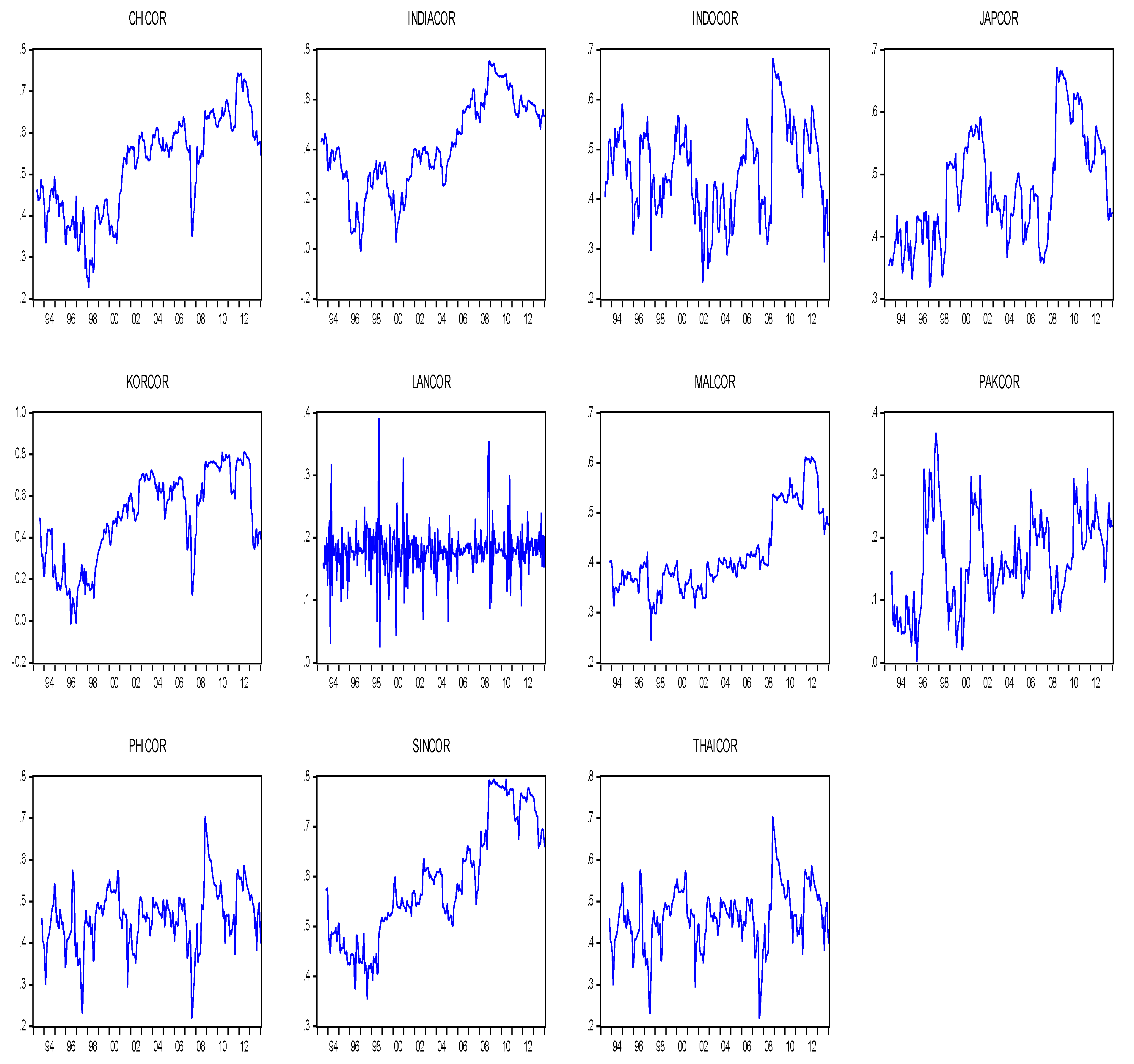
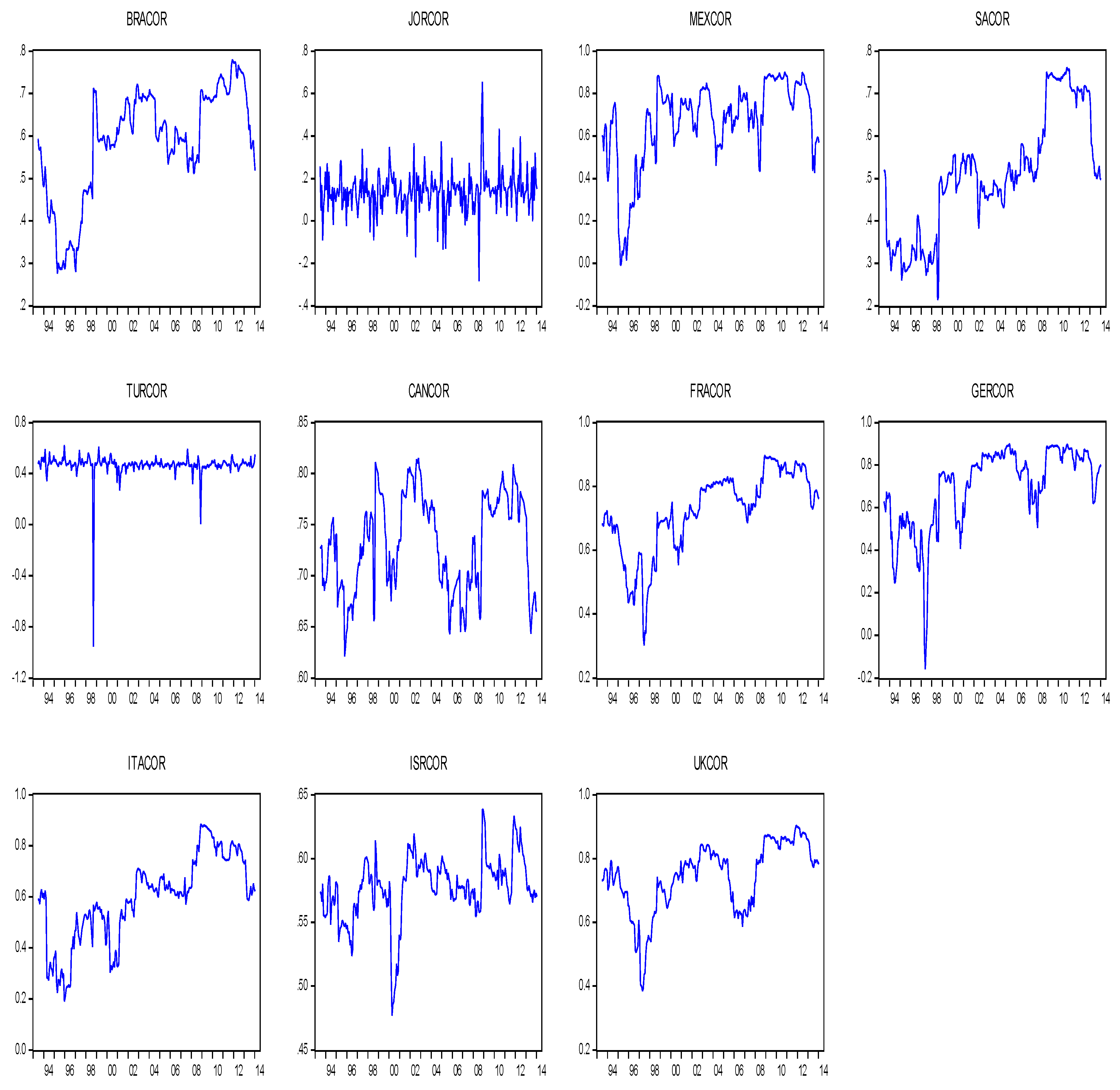
Our estimations suggested that all 24 pairwise correlations are time-varying (see Figure 1). The monthly and daily correlations averages are posted in panels 1 and 2 of

Table 1. Dynamic correlations with the US.

Panel 1: Monthly Correlations
Developed	Canada	France	Germany	Italy	Japan	UK
Cor	0.73	0.72	0.7	0.59	0.48	0.74
p-values	0.00	0.00	0.00	0.00	0.00	0.00
ARCH	0.36	0.16	0.20	0.12	0.07
p-values	0.03	0.03	0.02	0.13	0.18
GARCH	0.59	0.78	0.77	0.85	0.87
p-values	0.00	0.00	0.00	0.00	0.00
Emerging	Brazil	China	India	Israel	Malaysia	Taiwan	Singapore	Korea
Cor	0.58	0.51	0.42	0.58	0.42	0.49	0.6	0.49
p-values	0.00	0.00	0.00	0.00	0.00	0.00	0.00	0.00
ARCH	0.22	0.24	0.09	0.15	0.24	0.10	0.18	0.20
p-values	0.02	0.00	0.15	0.04	0.11	0.05	0.05	0.01
GARCH	0.61	0.71	0.79	0.79	0.73	0.87	0.80	0.79
p-values	0.00	0.00	0.00	0.00	0.00	0.00	0.00	0.00
Frontier	Argentina	Indonesia	Jordan	Mexico	Pakistan	Philippines	Sri Lanka	SA	Thailand	Turkey
Cor	0.47	0.45	0.58	0.66	0.16	0.43	0.18	0.58	0.46	0.47
p-values	0.00	0.00	0.00	0.00	0.00	0.00	0.00	0.00	0.00	0.00
ARCH	0.18	0.29	0.20	0.19	0.14	0.12	0.14	0.23	0.14	0.05
p-values	0.07	0.20	0.08	0.09	0.04	0.13	0.12	0.08	0.10	0.14
GARCH	0.62	0.63	0.64	0.75	0.82	0.81	0.60	0.51	0.80	0.93
p-values	0.00	0.02	0.00	0.00	0.00	0.00	0.14	0.00	0.00	0.00
Panel 2: Daily Correlations
Developed	Canada	France	Germany	Italy	Japan	UK
Cor	0.61	0.43	0.41	0.37	0.05	0.42
p-values	0.00	0.00	0.00	0.00	0.00	0.00
ARCH	0.07	0.07	0.08	0.08	0.77	0.07
p-values	0	0	0	0	0	0
GARCH	0.93	0.93	0.92	0.92	-0.81	0.92
p-values	0.00	0.00	0.00	0.00	0.00	0.00
Emerging	Brazil	India	Israel	Malaysia	Taiwan	Singapore	Korea
Cor	0.47	0.13	0.28	0.08	0.08	0.18	0.12
p-values	0.00	0.00	0.00	0.00	0.00	0.00	0.00
ARCH	0.10	0.10	0.06	0.06	0.06	0.10	0.07
p-values	0.00	0.00	0.00	0.00	0.00	0.00	0.00
GARCH	0.89	0.88	0.93	0.94	0.94	0.89	0.93
p-values	0.00	0.00	0.00	0.00	0.00	0.00	0.00
Frontier	Argentina	Indonesia	Jordan	Mexico	Pakistan	Sri Lanka	S. Africa	Turkey
Cor	0.41	0.08	0.01	0.55	0.03	0.02	0.24	0.17
p-values	0.00	0.00	0.00	0.00	0.00	0.00	0.00	0.00
ARCH	0.13	0.09	0.05	0.10	0.13	0.08	0.08	0.09
p-values	0.00	0.00	0.00	0.00	0.00	0.00	0.00	0.00
GARCH	0.84	0.91	0.94	0.88	0.85	0.91	0.91	0.90
p-values	0.00	0.00	0.00	0.00	0.00	0.00	0.00	0.00

Notes: Here, the dynamic conditional correlation mean estimates for the 24 nations against the US are reported for monthly and daily frequencies over the period 1993:01–2014:01. These are the correlations of the innovations (or abnormal return) derived from the autoregressive (AR(1)) moving average (MA(1))-generalized autoregressive conditional heteroskedasticity (GARCH)(1,1)-dynamic conditional correlation (DCC) or AR(1)-GARCH(1,1)-DCC models of market returns of the US and the other nation. The p-values corresponding to the test with the null that DCC mean is zero.

, respectively. We also noted the ARCH and GARCH effects for the two data frequencies. We noticed that both or one of the effects were statistically significant for all cases, suggesting that the DCC is appropriate. We noticed a big difference in the size of the correlations between the two frequencies—the monthly correlations were found to be much larger than the daily correlations for all MSCI returns examined here. This result is consistent with Narayan et al. (2014). For selected countries, the daily correlations with the US were found to be very low—close to ten per cent: Japan, India, Malaysia, Korea, Indonesia, Jordon, Pakistan, and Sri Lanka. These were also the lowest of the lot examined.

Focusing just on monthly correlations, we found that the US stock returns were most strongly integrated with the developed markets, with correlations of more than 70%. The Japanese market was the only exception; its correlation with the US market over the study period was found to be 48%. This was less than the correlations of the US with some of the emerging markets in the range of 50% to 60% (Brazil, China, Israel, Singapore, and South Korea). Some frontier markets also displayed greater integration with the US, for example, Mexico (66%) and Jordan (58%). However, frontier markets, such as Pakistan and Sri Lanka, revealed less than 20% integration with the US market, and those of the Philippines, Thailand, South Africa, Argentina, Thailand, and Turkey fell in the range of 43% to 47% integration.

Figure 1 reveals the correlations over time. Some markets (China, South Korea, Brazil, Mexico, and South Africa) saw higher correlations with the US by the end of the study period than at the start of the study period. More importantly, correlations were higher around the GFC, although we notice three distinct patterns as to how the pairwise correlations evolved in the GFC and post-GFC periods. We noticed a spike for frontier markets (Jordan and Sri Lanka) and a sudden increase followed by a gradual fall for Japan, some emerging markets (China, India, and Israel), and some frontier markets (Indonesia, Philippines, and Thailand). For some emerging (Singapore and Korea) and developed (Canada, France, Germany, Italy, and the UK) markets, a sharp increase in correlations plateaued before falling.

4. The Market Correlations and Correlation Volatility Response to Domestic and Foreign Shocks

4.1. The Multivariate EGARCH Model

To examine the determinants of correlations and correlation volatility over time, we used the multivariate EGARCH approach, similar to Koutmos and Booth (1995) and Booth et al. (1997). Equation (1) is the mean equation with ${\epsilon }_t={\delta }_t{z}_t$, where $z_t$ is standard Gaussian.

$$cor{r}_{ij,t}={\theta }_t+{\vartheta }_1{ϵ}_{i,t}+{\vartheta }_2{ϵ}_{j,t}+{\vartheta }_{3}F{C}_t+{\epsilon }_t,$$

(1)

where, $cor{r}_{ij,t}$ is the time-varying correlation between countries $i$ and $j$ at time, $t$; ${\theta }_t$ is the intercept and $\vartheta$ are the parameters to be estimated; and $FC$ is the global financial crisis variable. ${ϵ}_{i,t}$ and ${ϵ}_{j,t}$ are the return innovations or shocks from a market in country i, (one of the 24 nations that we refer to as domestic) and country j (where j is the US). In the pairwise correlation between the US and China, for instance, the US stock market is the source of foreign return innovations and the Chinese stock market is the source of domestic return innovations. These return innovations at time t are derived using the EGARCH model:

$${ϵ}_{k,t}=r_{k,t}-{\mu }_{k,t},\mathrm{for}k=i, j,$$

(2)

where, $r_{k,t}$ is the return of country i or j and ${\mu }_{k,t}$ is its conditional mean.

The conditional variance of the EGARCH model (1, 1) for the correlations is:

$$\ln {\delta }_{ij,t}^2=\omega +{\alpha }_1\left[\frac{\left|{\epsilon }_{t-1}\right|}{\left|\sqrt{{\delta }_{ij,t-1}^2}\right|}\right]+{\lambda }_1\frac{{\epsilon }_{t-1}}{\sqrt{{\delta }_{ij,t-1}^2}}+{\beta }_1\ln \left({\delta }_{t-1}^2\right).$$

(3)

The volatility shocks from the country i or j stock markets, derived following Jane and Ding (2009), are nested in Equation (3):

$$\ln {\delta }_{ij,t}^2=\omega +{\alpha }_1\left[\frac{\left|{\epsilon }_{t-1}\right|}{\left|\sqrt{{\delta }_{ij,t-1}^2}\right|}\right]+{\lambda }_1\frac{{\epsilon }_{t-1}}{\sqrt{{\delta }_{ij,t-1}^2}}+f_i\left(Z_{i,t-1}\right)+f_j\left(Z_{j,t-1}\right)+{\beta }_1\ln \left({\delta }_{ij,t-1}^2\right),$$

(4)

$$f_i\left(Z_{i,t}\right)={\gamma }_i\left(\left|Z_{i,t}\right|-E\left(\left|Z_{i,t}\right|\right)\right)+{\phi }_k\left(Z_{i,t}\right),$$

(5)

$$f_j\left(Z_{j,t}\right)={\gamma }_j\left(\left|Z_{j,t}\right|-E\left(\left|Z_{j,t}\right|\right)\right)+{\phi }_j\left(Z_{j,t}\right),$$

(6)

where, $Z_i$ is the standardised innovation in one of the 24 domestic stock markets, derived as $Z_i={ϵ}_{i,t}/{\sigma }_{i,t}$; $Z_j$ is the standardised innovation in the US nation, derived as $Z_j={ϵ}_{j,t}/{\sigma }_{j,t}$. ${\delta }_t^2$ is the conditional variance. ${\epsilon }_{t-1}$ is the residuals derived from Equation (1); $\omega$ is the constant; and ${\alpha }_1$ and ${\beta }_1$ signify the ARCH and GARCH effects, respectively. ${\beta }_1$ captures persistence of the correlation volatility. ${\lambda }_1$ gauges the overall leverage or asymmetric effect. The ${\lambda }_1$ is significant and less than 0 for negative asymmetry; and ${\lambda }_1$ is significant and greater than 0 for positive asymmetry; and insignificant for symmetry.

On the other hand, the asymmetric effects of standardized innovations from the stock markets i and j are measured by partial derivatives for $f_i$ and $f_j$ from Equations (5) and (6) respectively (Jane and Ding 2009). The leverage effect associated with market i, for instance, is measured by the ratio $\left|-{\gamma }_i+{\phi }_i\right|/\left({\gamma }_i+{\phi }_i\right)$. The ratio is greater than, equal to, or less than 1 for negative asymmetry, symmetry, and positive asymmetry respectively.

The total effect of shocks from market i is measured by $\left({\gamma }_{i+}{\phi }_i\right)$ for a unit increment of positive innovation and $\left(-{\gamma }_{i+}{\phi }_i\right)$ for a unit increment of negative innovation. The terms ${\gamma }_i\left(\left|Z_{i,t}\right|-E\left(\left|Z_{i,t}\right|\right)\right)$ or ${\gamma }_j\left(\left|Z_{j,t}\right|-E\left(\left|Z_{j,t}\right|\right)\right)$ measure the size effects while ${\phi }_k\left(Z_{i,t}\right)$ or ${\phi }_j\left(Z_{j,t}\right)$ measure the sign effects.

4.2. Empirical Results: The Influence of Domestic and Foreign Stock Market Shocks on Correlations (Equation (1))

The impact of market-return-based domestic and the US shocks on the correlations between the US and each of the 24 countries are discussed here. We estimated Equation (1) using monthly as well as daily data over the same time period. The multivariate EGARCH are presented in

Table 2. Effects of return and volatility shocks and the financial crisis: Developed countries and the US.

Dependent	Correlations			Volatility of Correlations
Independent Variables				ARCH	Total Leverage	GARCH	Domestic Volatility (Size)	Domestic Volatility (Sign)	US Volatility (Size)	US Volatility (Sign)		Domestic Volatility (Total)	US Volatility (Total)	Domestic Leverage ((Total))	US Leverage ((Total))
Independent Variables	Domestic	US	FC	${\mathit{\alpha }}_{\mathit{i}\mathit{j}}$	${\mathit{\lambda }}_{\mathit{i}\mathit{j}}$	${\mathit{\beta }}_{\mathit{i}\mathit{j}}$	${\mathit{\gamma }}_{\mathit{i}}$	${\mathit{\phi }}_{\mathit{i}}$	${\mathit{\gamma }}_{\mathit{j}}$	${\mathit{\phi }}_{\mathit{j}}$	R2	Vspi	Vspj	Levei	Levej
Panel 1: Monthly Frequency
Canada	−0.001 ***	0.000	0.025 ***	1.119 ***	0.088	0.638 ***	−0.044 ***	−0.162	0.083	0.2	−0.025	−0.206	0.283	−0.573	0.413
	0.015	0.982	0.000	0.000	0.272	0.000	0.714	0.421	0.543	0.310		0.331	0.196	0.602	0.632
France	0.000	0.000	0.000	0.784 ***	0.326	0.035	1.505 ***	−0.132	1.505 ***	0.346	−0.059	1.373 ***	1.851 ***	1.192 ***	0.626 ***
	0.269	0.906	0.927	0.003	0.058	0.702	0.000	0.644	0.000	0.189		0.000	0.000	0.009	0.010
Germany	0.001	0.000	0.000	0.19	0.017	−0.199 ***	1.033 ***	0.252	1.768 ***	−0.094	−0.072	1.285 ***	1.674 ***	0.608	1.112 ***
	0.095	0.707	0.932	0.423	0.920	0.002	0.000	0.441	0.000	0.776		0.007	0.001	0.126	0.009
Italy	0.001 ***	0.000	0.001	0.729 ***	0.256 ***	−0.058	1.624 ***	−0.028	1.702 ***	−0.083	−0.03	1.929 ***	1.797 ****	0.793 ***	1.140 ***
	0.000	0.189	0.703	0.000	0.009	0.185	0.000	0.873	0.000	0.563		0.000	0.000	0.000	0.000
Japan	0.001 ***	−0.001	−0.001	0.172	0.111	−0.066	1.729 ***	0.2	1.923 ***	−0.126	−0.007	1.596 ***	1.619 ***	1.035 ***	1.103 ***
	0.013	0.065	0.302	0.247	0.181	0.155	0.000	0.162	0.000	0.402		0.000	0.000	0.000	0.000
UK	0.001	−0.001	0.001	0.369	0.042	−0.027	1.139 ***	0.067	1.544 ***	0.211	−0.022	1.206 ***	1.755 ***	0.889	0.760 ***
	0.169	0.173	0.406	0.072	0.770	0.738	0.000	0.832	0.000	0.500		0.010	0.000	0.072	0.015
Panel 2: Daily Frequency
Canada	−0.001	−0.001	0.088 ***	1.309 ***	−0.041	0.817	−0.011	−0.020	−0.001	−0.014	0.07	−0.031	−0.015	−0.306	−0.895
	0.211	0.501	0.000	0.000	0.183	0.000	0.586	0.273	0.986	0.406		0.319	0.750	0.702	0.873
Fra	0.000	0.000	0.000	0.131 ***	−0.032	0.938	−0.118 ***	−0.044	−0.165 ***	−0.117 ***	0.00	−0.162 ***	−0.281 ***	−0.462	−0.170
	0.769	0.687	0.116	0.000	0.036	0.000	0.006	0.247	0.002	0.001		0.003	0.000	0.223	0.339
Ger	0.000	0.000	0.000	0.112 ***	−0.035	0.980	−0.089 ***	0.000	−0.147 ***	−0.094 ***	0.00	−0.089	−0.241 ***	−0.999	−0.219
	0.394	0.374	0.394	0.002	0.196	0.000	0.044	0.999	0.001	0.001		0.068	0.000	0.105	0.237
Ita	0.000	0.000	0.001	0.126 ***	−0.001	0.912	−0.129 ***	−0.028	−0.164 ***	−0.156 ***	0.00	−0.157 ***	−0.320 ***	−0.642	−0.025
	0.324	0.510	0.191	0.000	0.981	0.000	0.005	0.306	0.000	0.000		0.003	0.000	0.035	0.869
Jap	0.000 ***	0.000	−0.019 ***	1.861 ***	0.008	0.849	−0.001	−0.016 ***	−0.001	−0.021 ***	0.04	−0.018	−0.021	−0.862	−0.915
	0.004	0.032	0.000	0.000	0.426	0.000	0.925	0.029	0.947	0.018		0.223	0.168	0.525	0.455
UK	0.000	0.000	0.000	0.143 ***	−0.009	0.864	−0.169	−0.050	−0.214	−0.206 ***	0.00	−0.219 ***	−0.419 ***	−0.546	−0.018
	0.553	0.609	0.034	0.002	0.729	0.000	0.080	0.268	0.019	0.000		0.030	0.000	0.162	0.932

Notes: The figures in italics are the corresponding p-values for the coefficients reported. *** denote the level of significance at 1 percent.

,

Table 3. Effects of domestic and foreign shocks and the financial crisis: Emerging markets and the US.

	Correlations			Volatility of Correlations
				ARCH	Total Leverage	GARCH	Domestic Return Volatility Size	Domestic Return Volatility Sign	US Return Volatility Size	US Return Volatility Sign		Total Domestic Return Volatility	Total US Return Volatility	Leverage Effects (Domestic Market)	Leverage Effects (US Market)
	Domestic	US	FC	${\mathit{\alpha }}_{\mathit{i}\mathit{j}}$	${\mathit{\lambda }}_{\mathit{i}\mathit{j}}$	${\mathit{\beta }}_{\mathit{i}\mathit{j}}$	${\mathit{\gamma }}_{\mathit{i}}$	${\mathit{\phi }}_{\mathit{i}}$	${\mathit{\gamma }}_{\mathit{j}}$	${\mathit{\phi }}_{\mathit{j}}$	R2	Vspi	Vspj	Levei	Levej
Panel 1: Monthly Frequency
Brazil	0.000	0.000	0.000	0.26	−0.062	−0.023	1.669	0.123	1.921	0.069	−0.037	−0.156 ***	1.99 ***	−0.141 ***	0.824 ***
	0.320	0.915	0.211	0.274	0.654	0.684	0.000	0.580	0.000	0.758		0.000	0.000	0.000	0.000
China	0.000 ***	0.000	0.001	0.356	0.112	0.041	1.807 ***	0.002	2.163 ***	0.028	−0.011	1.809 ***	2.191 ***	0.998 ***	0.974 ***
	0.038	0.306	0.283	0.126	0.411	0.342	0.000	0.989	0.000	0.861		0.000	0.000	0.000	0.000
India	0.000 ***	0.000	0.001	0.280 ***	0.106	−0.062	2.073 ***	0.049	2.035 ***	−0.1	−0.009	2.122 ***	1.935 ***	0.954 ***	1.103 ***
	0.020	0.250	0.597	0.034	0.092	0.099	0.000	0.569	0.000	0.315		0.000	0.000	0.000	0.000
Israel	0.000	0.000	0.006 ***	1.193 ***	−0.009	0.705 ***	0.697 ***	0.041	0.280 ***	−0.15	0.01	0.738 **	0.13	0.889 **	3.308
	0.429	0.880	0.000	0.000	0.887	0.000	0.001	0.798	0.008	0.268		0.015	0.506	0.027	0.537
Malaysia	0.000	0.000	0.000	0.248	0.062	−0.055	1.941 ***	−0.214 ***	2.264 ***	0.221 ***	−0.047	1.727 ***	2.485 ***	1.248 ***	0.822 ***
	0.393	0.059	0.988	0.100	0.379	0.121	0.000	0.037	0.000	0.036		0.000	0.000	0.000	0.000
Taiwan	0.000	−0.001 **	0.001	0.580 ***	0.330 ***	−0.072	1.874 ***	0.18	2.324 ***	0.162	0.019	2.054 ***	2.486 **	0.825 ***	0.870 ***
	0.516	0.050	0.283	0.000	0.005	0.142	0.000	0.251	0.000	0.338		0.000	0.000	0.000	0.000
Singapore	0.000	0.000	0.001	0.843 ***	0.442 ***	−0.039	1.825 ***	−0.176	2.076 ***	0.126	−0.054	1.649 ***	2.202 ***	1.213 ***	0.886 ***
	0.310	0.308	0.114	0.000	0.000	0.490	0.000	0.331	0.000	0.494		0.000	0.000	0.000	0.000
Korea	0.000	0.000	0.003	0.26	0.047	−0.220 ***	1.934 ***	0.082	2.170 ***	0.105	−0.009	2.016 ***	2.275 ***	0.919 ***	0.908 ***
	0.262	0.484	0.247	0.162	0.648	0.000	0.000	0.599	0.000	0.521		0.000	0.000	0.000	0.000
Panel 2: Daily Frequency
Brazil	−0.001	0.000	0.140 ***	1.251 ***	−0.030	0.802 ***	−0.045	−0.007	−0.063 ***	−0.032	0.08	−0.053	−0.094 ***	−0.721	−0.331
	0.480	0.726	0.000	0.000	0.063	0.000	0.175	0.679	0.010	0.100		0.056	0.006	0.299	0.251
India	0.001	0.001	0.001	0.531 ***	−0.051	0.874 ***	−0.174	−0.118 **	−0.177 ***	−0.127	0.00	−0.292 ***	−0.304 ***	−0.193	−0.166
	0.165	0.125	0.481	0.000	0.083	0.000	0.070	0.041	0.006	0.011		0.000	0.000	0.678	0.617
Israel	0.000	0.000	0.000	0.187	0.013	0.383 ***	−0.218 ***	−0.111 **	0.067	−0.351 ***	0.00	−0.329 ***	−0.284	−0.326	−1.472
	0.320	0.159	0.873	0.188	0.905	0.003	0.026	0.052	0.624	0.000		0.006	0.011	0.249	0.188
Malay	−0.001 ***	0.000 ***	0.003 ***	1.510 ***	−0.011	0.919 ***	−0.028 ***	0.001	−0.007	−0.011	−0.03	−0.027	−0.018	−1.096	−0.234
	0.000	0.011	0.000	0.000	0.164	0.000	0.031	0.895	0.622	0.183		0.090	0.247	0.149	0.824
Taiwan	−0.001 ***	0.000	0.000	0.179 ***	−0.050	0.625 ***	−0.260	−0.097	−0.424	−0.215 ***	0.00	−0.356	−0.640	−0.458	−0.326
	0.001	0.649	0.647	0.001	0.160	0.000	0.415	0.187	0.272	0.000		0.213	0.104	0.509	0.436
Singapore	0.000	0.000	0.000	0.058	−0.079 ***	0.869 ***	−0.111 **	−0.081 ***	−0.097	−0.157 ***	0.00	−0.192 ***	−0.253 ***	−0.155	−0.238
	0.889	0.228	0.157	0.142	0.003	0.000	0.052	0.011	0.145	0.001		0.001	0.011	0.655	0.387
Korea	0.000	0.000	0.000	0.213 ***	0.008	0.666 ***	−0.184	−0.066	−0.198	−0.213 ***	0.00	−0.249	−0.411 **	−0.474	−0.036
	0.549	0.092	0.641	0.002	0.846	0.000	0.080	0.168	0.219	0.001		0.058	0.021	0.089	0.932

Notes: The figures in italics are the corresponding p-values for the coefficients reported. *** and ** denote the level of significance at 1 and 5 percent.

and

Table 4. Effects of return and volatility shocks and the financial crisis: Frontier markets and the US (Panel 1: monthly data).

Dependent	Correlations			Volatility of Correlations
Independent				ARCH	Total Leverage	GARCH	Domestic Volatility (Size)	Domestic Volatility (Sign)	US Volatility (Size)	US Volatility (Sign)		Domestic Volatility (Total)	US Volatility (Total)	Domestic Leverage (Total)	US Leverage (Total)
Independent	Domestic	US	FC	${\mathit{\alpha }}_{\mathit{i}\mathit{j}}$	${\mathit{\lambda }}_{\mathit{i}\mathit{j}}$	${\mathit{\beta }}_{\mathit{i}\mathit{j}}$	${\mathit{\gamma }}_{\mathit{i}}$	${\mathit{\phi }}_{\mathit{i}}$	${\mathit{\gamma }}_{\mathit{j}}$	${\mathit{\phi }}_{\mathit{j}}$	R2	Vspi	Vspj	Levei	Levej
Argentina	0.001 ***	−0.001	0.005	0.668 ***	0.067	0.245 ***	1.507 ***	0.226 ***	1.285 ***	−0.241 **	−0.06	1.733 ***	1.044 ***	0.739 ***	1.462 ***
	0.001	0.092	0.053	0.000	0.487	0.000	0.000	0.045	0.000	0.052		0.000	0.000	0.000	0.000
Indonesia	0.000	0.000	−0.071 ***	1.382 ***	−0.032	0.647 ***	0.298 ***	−0.026	0.424 ***	−0.02	−0.146	0.272	0.404 **	1.191	1.099 **
	0.107	0.665	0.000	0.000	0.724	0.000	0.008	0.746	0.000	0.833		0.091	0.033	0.084	0.032
Jordan	0.003	−0.004	0.009	0.676	−0.107	0.442	0.895	0.058	0.962	0.044	0.007	0.922 ***	1.006 ***	−0.875 ***	5.943
	0.415	0.012	0.349	0.000	0.149	0.000	0.000	0.477	0.000	0.635		0.000	0.000	0.000	0.682
Mexico	−0.002	0.002	−0.034	1.509	−0.254	0.726	0.306	−0.064	−0.164	0.23	−0.297	0.242	0.066	−1.524	0.240
	0.001	0.025	0.000	0.000	0.006	0.000	0.003	0.530	0.125	0.009		0.174	0.673	0.200	0.623
Pakistan	0.000	0.000	0.006 ***	1.563 ***	0.122	0.521 ***	0.741 ***	−0.191 ***	0.827 ***	0.066	−0.006	0.550 ***	0.893 ***	1.695 ***	0.852 ***
	0.175	0.661	0.014	0.000	0.096	0.000	0.000	0.004	0.000	0.273		0.000	0.000	0.000	0.000
Philippines	0.000	0.000	−0.032 ***	1.302 ***	0.075	0.380 ***	0.005	−0.003	0.605 ***	−0.029	−0.012	0.002	0.576 ***	4.000	1.101 ***
	0.563	0.894	0.000	0.000	0.524	0.000	0.969	0.974	0.000	0.782		0.989	0.001	0.989	0.005
Sri Lanka	0.000 ***	0.000	0.002	0.603 ***	−0.149 ***	0.485 ***	1.567 ***	−0.12	1.558 ***	0.013	−0.039	1.447 ***	1.571 ***	1.166 ***	0.983 ***
	0.008	0.732	0.330	0.000	0.026	0.000	0.000	0.122	0.000	0.870		0.000	0.000	0.000	0.000
South Africa	0.000	0.000	0.06	1.574	0.022	0.022 ***	0.179	−0.14	0.125	0.077	−0.037	0.039	0.202	8.278	−0.912 ***
	0.996	0.212	0.000	0.000	0.800	0.000	0.042	0.017	0.116	0.260		0.712	0.069	0.701	0.000
Thailand	0.000	−0.001	−0.031 ***	1.282 ***	0.084	0.478 ***	0.627 ***	0.196 ***	0.475 ***	0.068	0	0.823 ***	0.543 ***	0.524 ***	0.750 ***
	0.916	0.242	0.000	0.000	0.426	0.000	0.000	0.038	0.000	0.554		0.000	0.008	0.000	0.030
Turkey	0.000	0.000	−0.006 ***	0.122	0.244 ***	0.160 ***	1.680 ***	0.029	1.916 ***	0.051	−0.018	1.709 ***	1.967 ***	0.966 ***	0.948 ***
	0.163	0.839	0.002	0.398	0.005	0.005	0.000	0.834	0.000	0.729		0.000	0.000	0.000	0.000

Notes: The figures in italics are the corresponding p-values for the coefficients reported. *** and ** denote the level of significance at 1 and 5 percent.

with monthly and daily estimations reported in panels 1 and 2, respectively.

4.2.1. Monthly

We began by looking at the implications of foreign and domestic shocks on the correlations between the US and developed (Table 2), emerging (Table 3), or frontier (Table 4 and

Table 5. Effects of return and volatility shocks and the financial crisis: Frontier and the US stock markets (Panel 2: daily data).

Dependent Variable	Correlations			Volatility of Correlations
Independent Variables				ARCH	Total Leverage	GARCH	Domestic Volatility Size	Domestic Volatility Sign	US Volatility Size	US Volatility Sign		Total Domestic Volatility	Total US Volatility	Domestic Leverage ((Total))	US Leverage ((Total))
Independent Variables	Domestic Shocks	US Shocks	FC	${\mathit{\alpha }}_{\mathit{i}\mathit{j}}$	${\mathit{\lambda }}_{\mathit{i}\mathit{j}}$	${\mathit{\beta }}_{\mathit{i}\mathit{j}}$	${\mathit{\gamma }}_{\mathit{i}}$	${\mathit{\phi }}_{\mathit{i}}$	${\mathit{\gamma }}_{\mathit{j}}$	${\mathit{\phi }}_{\mathit{j}}$	R2	Vsp(i)	Vsp(j)	Leve(i)	Leve(j)
Argentina	0.004 ***	−0.003 ***	0.129 ***	1.429 ***	−0.055 ***	0.817 ***	−0.065 ***	0.010	0.017	−0.054 ***	0.07	−0.055 **	−0.037	−1.365 **	−1.900
	0.000	0.001	0.000	0.000	0.000	0.000	0.005	0.523	0.523	0.002		0.051	0.159	0.050	0.329
Indonesia	0.000	0.000	0.001 **	0.107 **	0.001	0.916 ***	−0.157 ***	−0.003	−0.149	−0.197 ***	0.00	−0.159 ***	−0.346 ***	−0.967 ***	−0.139
	0.835	0.924	0.036	0.016	0.976	0.000	0.001	0.921	0.008	0.000		0.003	0.000	0.003	0.464
Jordon	0.000	0.000	0.001	0.930 ***	−0.001	0.827 ***	−0.135 **	0.010	−0.086	−0.011	0.00	−0.125	−0.096	−1.158 ***	−0.779
	0.788	0.708	0.438	0.000	0.974	0.000	0.037	0.679	0.315	0.830		0.056	0.363	0.005	0.387
Mexico	0.000	0.000	0.074 ***	1.377 ***	−0.040 ***	0.846 ***	0.009	−0.036	−0.021	−0.017	0.08	−0.027	−0.038	−1.647	−0.101
	0.970	0.983	0.000	0.000	0.001	0.000	0.787	0.086	0.239	0.290		0.235	0.090	0.561	0.880
Pakistan	−0.003	−0.001	0.006	0.453 ***	−0.092 **	0.596 ***	−0.083	−0.200	−0.038	−0.347 ***	−0.03	−0.283	−0.385	−0.415	−0.803
	0.022	0.075	0.145	0.000	0.006	0.000	0.285	0.105	0.755	0.003		0.097	0.086	0.257	0.128
Sri Lanka	0.000	0.000	0.001 ***	1.036 ***	−0.021	0.788 ***	−0.027	0.001	0.006	−0.056 ***	0.01	−0.025	−0.050	−1.088	−1.243
	0.225	0.366	0.000	0.000	0.162	0.000	0.199	0.948	0.838	0.017		0.364	0.144	0.437	0.346
South Africa	0.000	0.000	0.000 **	0.121	0.092	0.764 ***	0.023	0.012	−0.176	−0.208 ***	0.00	0.035	−0.384	0.330	−0.084
	0.354	0.199	0.031	0.083	0.094	0.000	0.742	0.889	0.141	0.016		0.780	0.046	0.914	0.716
Turkey	0.000	0.000	0.001 ***	0.033	−0.004	−0.332 **	−0.123	−0.144 ***	0.294	−0.143	0.00	−0.266	0.150	−0.079	2.904
	0.292	0.168	0.006	0.648	0.944	0.020	0.390	0.011	0.147	0.105		0.096	0.322	0.892	0.114

Notes: The figures in italics are the corresponding p-values for the coefficients reported. *** and ** denote the level of significance at 1 and 5 percent.

) equity markets. Table 2, Table 3, Table 4 and Table 5, panel 1 (columns 2–4), which report the estimated coefficients (and corresponding t-statistics) from the mean models, show more cases of significant domestic (country i) shocks (captured by ${\theta }_1$) than US shocks (captured by ${\theta }_2$). Domestic shocks were found to influence nine out of 24 country-wise correlations. Shocks originating from domestic stock markets in China, India, Japan, Sri Lanka, Argentina, Mexico, and Italy were found to have positive effects on their stock market correlations with the US. Innovations from Brazil and Canada markets reduced their market correlations with their counterparts in the US.

Shocks originating from the US stock market were found to only have a significant effect on their correlations with Taiwan, Brazil, and Mexico. While the influence of the US stock market shocks increased the correlations with Brazil, those with respect to the Taiwan and Mexico markets were negative.

We found that eight of the pairwise correlations responded significantly to the financial crisis variable (captured by ${\theta }_3$). However, unlike several studies (Johansson 2011; Arouri and Jawadi 2010), which showed a positive effect of the financial crisis on stock market integration, we found that the effects can be mixed. A strong prevalence of negative effects on US correlations was found with four frontier markets (Indonesia, Philippines, Thailand, and Turkey); and one emerging market, Brazil. The US correlations with frontier markets in Pakistan and Israel and one developed market (Canada) were found to increase with financial crises.

4.2.2. Daily

The daily results are presented in Table 2, Table 3, Table 4 and Table 5, panel 2, columns 2–4. Unlike the monthly analysis, return-based-shocks from both the US and/or domestic stock returns did not matter for the determination of “daily correlations”, for most cases. The set of countries that showed significant effects was also different from that of the monthly results. Both domestic and US return spillovers were found to be significant determinants of correlations for two countries only, Malaysia and Argentina, while domestic return innovations were found to be the only determinant of Japan and Taiwan stock market correlations with the US.

The financial crisis variable was found to be an important determinant of correlations for nine countries, although in the monthly analysis, none of these showed this result, suggesting that the effect of the financial crisis on correlation is immediate and short-lived.

4.3. Impact of Domestic and Foreign Stock Market Volatility-Based Innovations on Correlation Volatility (Equation (4))

4.3.1. Monthly

The effects of US (or foreign) stock market return volatility shocks on correlation volatility are captured in columns 9 and 10 of Table 2, Table 3, Table 4 and Table 5, while the country-specific (for the corresponding country in the column 1) volatility effects are captured in columns 7 and 8 of Table 2, Table 3, Table 4 and Table 5. These results were derived from estimating Equation (3). The three key results that emerged from the correlation variance equation were as follows.

First, for the US and country-specific return volatility, in most cases, the size (shown by $\gamma )$ (and not sign ($\phi$)) of the innovations was the most important determinant of correlation volatility. A similar finding was reported by Koutmos and Booth (1995) in their study of the volatility of returns.

Second, in terms of the impacts of the total volatility shocks from the two sources (derived as ($\gamma +\phi ),$ in columns 9 and 10 for the US, vsp(j) and in columns 7 and 8 for the nation listed in column 1, vsp(i), most of the time, volatility shocks originating in the US seem to have a stronger effect on the volatility of the correlations than those of domestic origin. These results are similar to those from other studies that showed that the US is an important source of stock market volatility (see Wei et al. 1995; Kim and Rogers 1995; Theodossiou and Lee 1993).

It is also noteworthy that the US stock market volatility effects were found to be stronger and much more prevalent than the US return effects. This finding is consistent with multivariate studies based on stock returns, which find that international volatility shocks are also more prominent determinants of stock market return and their volatility. An early study by Kyle (1985) suggested that much of the information contained in other market’s price movements could be revealed in the volatility of stock prices, rather than in the price. Kim and Rogers (1995) found that US and Japanese volatility shocks have a strong influence on the returns of the Korean stock market.

The country-specific volatility innovations originating in India, Italy, Thailand, Argentina, Sri Lanka, Israel, and Mexico were, however, found to have stronger effects on the volatility of their correlations with the US. It seems that the importance of domestic stock market return and volatility innovations for some frontier markets, namely, India, Sri Lanka, and Argentina, should not be under-estimated.

The third key result is evidence of the leverage effect on the volatility, that is, the tendency that the volatility of correlations is higher after negative shocks than after positive shocks is limited. Asymmetric effects due to shocks originating from the domestic country within the pairwise relations were measured by the ratio $\left|-{\gamma }_i+{\phi }_i\right|/\left({\gamma }_i+{\phi }_i\right)$. Asymmetric effects due to shocks originating from the US were measured by the ratio $\left|-{\gamma }_j+{\phi }_j\right|/\left({\gamma }_j+{\phi }_j\right)$. The domestic and US leverage effects correspond to levei and levej in columns 15 and 16, and these were calculated using columns 8–9 and 10–11, respectively, in Table 2, Table 3, Table 4 and Table 5.

The volatility of correlations between the stock markets of most countries and the US were found to be symmetric most of the time. While we noticed more cases of leverage effects when we studied domestic (16 cases) and foreign (20 cases) shocks separately (see columns 15 and 16, Table 2 and Table 3; panel 1; Table 4 and Table 5), the overall leverage effects (column 6) were limited. The overall measure of the leverage effect (captured by ${\lambda }_1$) was significant and negative for the US correlations with Sri Lanka and Mexico. There were four cases of positive asymmetries (or ${\lambda }_1>0$ and significant)—the US correlations with Italy, Singapore, Taiwan, and Turkey. For these pairwise correlations, positive shocks were shown to have a greater impact on volatility than negative shocks. The lack of evidence on the leverage effect is inconsistent with the stock return literature. In section 4, we investigated whether the leverage effects could be found under bear market conditions.

4.3.2. Daily

The effects of daily domestic and US shocks on the correlation volatility are reported in Table 2, Table 3, Table 4 and Table 5, panel 2, and columns 8–9 and 10–11, respectively. Eight (nine) countries’ correlation volatility was found to be influenced by domestic (US) innovations—this was less than what was found using monthly data. For France, Italy, UK, India, Singapore, and Indonesia, the volatility of their abnormal return correlation with the US were found to be influenced by both US and domestic shocks. However, the US was found to be the only source of the correlation volatility of Germany, Brazil, and Korea, while the volatility of Israel’s correlation with the US was only affected by domestic (or Israel based volatility) shocks.

Evidence of the significant US sourced leverage effect with daily data was missing in this study (columns 15–16). There was strong evidence of symmetric shocks. Little evidence of positive asymmetry driven by domestic shocks was seen for Argentina, Indonesia, and Jordan. An overall negative asymmetric effect (displayed in column 6) was found for Singapore (–), Argentina (–), Mexico (–), and Pakistan (–).

4.4. Persistence of Market Synchronization Volatility

4.4.1. Monthly Data

Next, we examined the persistence of the correlation volatility. In explaining the implications of the persistence of correlations, Candelon et al. (2008) explained that if stock market synchronization has a lasting characteristic, and there is an increase in synchronization, then regulatory bodies probably need to configure their supervisory frameworks towards preserving the stability of their financial system for the long term in an effort to prevent a financial crisis. However, if the stronger co-movement between markets is transitory, then the prevention of these shocks and the reduction of their financial and economic effects become important (Candelon et al. 2008).

In a similar way, if diversification risk (or correlation volatility) is persistent, then this has implications for policy as well as investment. The persistence of correlation volatility was captured by ${\beta }_1$ (Table 2, Table 3, Table 4 and Table 5, panel 1, column 7). Our results suggest that for most correlation pairs, this coefficient was insignificant or closer to zero (if significant). This suggests that, for most cases, correlation volatility is not persistent at all. This transitory behavior can be seen in Figure 1 as well. These results suggest that, for most cases, the rise in synchronization only temporarily reduced the ability to diversify risk internationally. Nonetheless, there was some evidence that correlation volatility is persistent in the following pairs: US–Indonesia, US–Pakistan, US–Brazil; US–Israel, US–Canada, and US–UK. For the case of the US (non-US nations) cases, it would be worth looking at markets outside Indonesia, Pakistan, Brazil, Israel, Canada, and the UK (the US) in times when the correlations are higher.

4.4.2. Daily

Daily persistence was captured in column 7 of Table 2, Table 3, Table 4 and Table 5, panel 2. Some persistence should be expected when using daily data. Our results show that daily correlation volatilities were mainly persistent, more so than the monthly ones. This analysis provided further support for the claims made above.

4.5. Overall Implication

When we compared the results of the daily and monthly frequencies, the key findings were as follows. The correlations and their volatilities of most stock markets with the US were unaffected by aggregate US or domestic stock market shocks (related to returns or their volatilities, respectively) within a day or so. However, these shocks could become significant by a month. This means that in the case of portfolios with two international stocks, such as those examined here, gains in diversification and their risks were mainly unaffected by domestic or foreign shocks within a day. However, these were likely to change within a month. We also found that there was a lack of persistence in the influence of domestic and foreign shocks on diversification risk. This implies that shocks to diversification gains did not last for more than a month.

5. Bear Market Conditions

In the previous analysis, it was revealed that monthly market correlations (or portfolio gains) were influenced by domestic and US return shocks, although the chance of a significant effect of domestic shocks occurring was likely to be higher. Additionally, while domestic and US volatility shocks were closer in magnitude, it was the US market risk that seemed, most of the time, to be the key determinant of correlation volatility (or portfolio risk). Our analysis also revealed that the markets of India, Argentina, and Sri Lanka were predominantly determined by domestic market return and volatility shocks.

Daily returns data, on the other hand, showed relatively weak evidence of domestic or US return and volatility shocks on correlations. We found strong evidence of symmetric effects of volatility shocks. Given the irrelevance of aggregate return shocks and the limited evidence of volatility spillover effects on daily correlations with the US, we did not pursue further analysis using daily results. Our usage of monthly data (in the examination of asymmetric correlations from here on) also takes heed of the findings of Ang and Chen (2002)—the only study we found that estimated asymmetric correlations across frequencies. These authors estimated asymmetric correlations across daily, weekly, and monthly frequencies for size-based portfolios of US firms against the US market and found that correlations symmetries were greatest with monthly frequency.

Similarly, with monthly returns data, in the majority of the cases, we found that US and domestic shocks have symmetric effects on stock market correlations. This stands in sharp contrast to studies that show a strong presence of the leverage effect in the stock market. Koutmos and Booth (1995) in their study of the US, UK, and Japanese markets, in particular, used the multivariate EGARCH model to show that volatility shocks in a given market are much more pronounced when the news arriving from the last market to trade is bad. Furthermore, in their comparison of the pre- and post-October 1987 stock market crash, Koutmos and Booth (1995) found that the leverage effect became significant only in the post-stock market crash period. Cappiello et al. (2006) allowed for these asymmetric effects relating to the equity markets in the calculations of DCCs.

Some existing studies (such as Longin and Solnik 1995; Ang and Chen 2002; Narayan 2015) show evidence of asymmetry in the correlations—in particular, that conditional correlations increase strongly in bear markets but do not increase in bull markets. Ang and Chen (2002) also showed similar asymmetric correlations between US stocks and the US aggregate market, although they did not find a relationship between leverage and correlation asymmetries.

In line with existing evidence, we examined whether our results would change if volatility and return shocks picked up bear market features. In particular, would the US bear market-related return and volatility shocks continue to have a bigger impact on correlations, as indicated by previous literature? More importantly, given that the leverage effects are stylized by stock returns, would their presence be revealed during times when market news is mainly bad? Another important question is whether the volatility becomes persistent after bearish shocks.

We attempted to answer these questions by first distinguishing bear market features from that of a bull market for the US and the other 24 nations by using the two-region Markov switching model. We then developed return and volatility shocks before examining their influences on the pairwise dynamic conditional correlations.

5.1. Filtered Data on Bear Markets

To separate bear market features, we use a simple two-stage Markov-switching model following Chen (2009). In this model, the mean of returns,$r_t$, is subject to regime switching. Error variance is assumed to differ across the regimes. As a result, a two state mean/variance Markov-switching model of stock returns is:

$$r_t={\mu }_{st}+{ϵ}_t, {ϵ}_t~i.i.d.\left(0,{\sigma }_{st}^2\right),$$

(7)

where, ${\mu }_{st}$ and ${\sigma }_{st}^2$ are the regime-dependent mean and variance of $r_t$, respectively. If $s_t=m$, then the market is in regime $m$. We classified the two regimes as bull and bear markets so that when $s_t=0$ market is bear; and when $s_t=1$ market is bull. The stock return, following the two-state Markov process, has the following transition probability matrix:

$$P=\left[\begin{array}{cc}{p}^{00}& p^{01}\\ p^{10}& p^{11}\end{array}\right],$$

(8)

where, $p^{00}=P\left(s_t=0|s_{t-1}=0\right)$; $p^{11}=P\left(s_t=1|s_{t-1}=1\right)$; $p^{01}=1-p^{11}$; and $p^{10}=1-p^{00}$. Once the two regimes are statistically identified, the filtered probabilities for each state are computed. This indicates the probability of the bear (or bull) each month: ${\theta }_{j,t}=P\left(s_t=j|{\phi }_{t-1}\right)$, $j=\left\{0,1\right\}$.

Table 6. Bear and bull market features in selected Asian, other emerging, and some developed markets.

Countries	Bear Regime		Bull Regime		Transition Probabilities		Expected Duration
	Mean	Variance	Mean	Variance	Bear	Bull	Bear	Bull
Canada	−2.196	2.230 ***	1.475 ***	1.447 ***	0.869	0.964	7.6124	27.61
	0.205	0.000	0.000	0.000
France	−1.082	2.084 ***	1.418 ***	1.383 ***	0.950	0.971	20.092	35.0308
	0.264	0.000	0.000	0.000
Germany	−1.038	2.188 ***	1.829 ***	1.375 ***	0.973	0.960	36.678	25.0415
	0.288	0.000	0.000	0.000
Italy	−12.752 ***		1.076		0.368	0.961	1.5819	25.8124
	0.000		0.062
Japan	−0.299	1.859 ***	0.581	1.387 ***	0.983	0.978	59.7	45.1
	0.590	0.000	0.205	0.000
UK	−0.856	1.774 ***	1.343 ***	1.073 ***	0.941	0.954	16.985	21.8999
	0.199	0.000	0.000	0.000
US	0.114	1.709 ***	1.082 ***	0.857 ***	0.978	0.981	45.476	53.941
	0.807	0.000	0.000	0.000
China	−2.534	2.595 ***	1.500 ***	1.798	0.957	0.969	23.3	32.1
	0.079	0.000	0.009	0.000
Brazil	−4.810	2.972 ***	1.858 ***	2.131 ***	0.750	0.954	3.9967	21.6182
	0.251	0.000	0.006	0.000
India	−22.032 ***		0.821		0.466	0.993	1.9	151.1
	0.008		0.146
Israel	−0.665	1.347 ***	0.865 ***	0.462 ***	0.765	0.782	4.5848	4.25573
	0.147	0.000	0.000	0.001
Malaysia	−1.891	2.740 ***	0.899	1.649 ***	0.928	0.983	13.9	59.9
	0.416	0.000	0.044	0.000
Singapore	−0.757	2.420 ***	0.997 ***	1.432 ***	0.883	0.938	8.5	16.1
	0.540	0.000	0.011	0.000
S. Korea	−0.459	2.868 ***	0.847	1.914 ***	0.962	0.989	26.4	89.4
	0.849	0.000	0.103	0.000
Taiwan	−0.098	2.326 ***	0.759	1.675 ***	0.983	0.976	57.8	41.5
	0.877	0.000	0.202	0.000
Argentina	−9.558 ***	2.881 ***	2.263 ***	2.129 ***	0.749	0.944	3.9873	17.9946
	0.019	0.000	0.001	0.000
Indonesia	−3.531	3.056 ***	1.657 ***	2.035 ***	0.962	0.989	26.3	89.5
	0.206	0.000	0.005	0.000
Jordan	−0.583 ***	0.264 ***	0.612 ***	1.074 ***	0.877	0.893	8.1149	9.32911
	0.001	0.034	0.037	0.000
Mexico	−33.421 ***	2.078 ***	1.352 ***	1.984 ***	0.386	0.987	76.61	1.62986
	0.000	0.000	0.004	0.000
Pakistan	−5.239	3.070 ***	0.910	2.097 ***	0.829	0.975	5.8	39.7
	0.256	0.000	0.124	0.000
Philippines	−18.454 ***		0.848		0.542	0.984	2.2	61.0
	0.007		0.135
S. Africa	−6.645	2.753 ***	1.115 ***	1.929 ***	0.765	0.984	4.2634	62.9653
	0.276	0.000	0.020	0.000
Sri Lanka	−0.579	1.782 ***	2.249	2.699 ***	0.863	0.718	7.3	3.5
	0.570	0.000	0.234	0.000
Thailand	−2.834	2.844 ***	1.281 **	1.960 ***	0.945	0.978	18.1	46.3
	0.179	0.000	0.039	0.000
Turkey	−0.994	2.961 ***	1.981	2.373 ***	0.959	0.966	24.398	29.7673
	0.639	0.000	0.068	0.000

Notes: The figures in italics are the corresponding p-values for the coefficients reported. *** and ** denote the level of significance at 1 and 5 percent.

presents the Markov-switching models of $r_t$ for the US and other markets examined. During the period 1993:01 to 2014:01, one developed market, Italy (−13%), and some frontier markets (Mexico (−33%), followed by India (−22%), the Philippines (−18%), Argentina (−10%), and Pakistan (−5%)) registered the lowest mean returns in the bear phase. Others ranged between 0.1% (the US) and −5% (Brazil). For the same period, when markets were bull, Sri Lanka and Argentina markets registered the highest average return, just modestly above 2%. Consistent with previous studies, we found bear markets to be more volatile than bull markets (see, for instance, Chen 2009; Gander 2011; Longin and Solnik 2001). For our study period, the only exception to the rule was Sri Lanka.

Transition probabilities indicate that for most markets there was a relatively higher probability of remaining in the bull or bear regimes, suggesting that these regimes were fairly persistent. However, India, the Philippines, Mexico, and Italy show relatively lower probabilities of remaining in bear regimes. In fact, for India, Mexico, and Italy, the transition from bull to bear took a relatively higher probability than the probability of being in a bear state. The probabilities for the transition from bull to bear for India, the Philippines, Mexico, and Italy were 0.534 (1 − 0.466); 0.438; 0.614; and 0.632, respectively. Furthermore, the expected duration of a bear market ranged from 77 months (Mexico) to 2 months (Italy), while those for a bull market range from 151 months (India) to 3.5 months (Sri Lanka). Taken together, it seemed some markets were more persistent during a bull phase than a bear phase—these were India, Indonesia, Korea, South Africa, the Philippines, Malaysia, the US, Thailand, France, China, Turkey, Canada, Italy, the UK, Brazil, Argentina, Singapore, and Jordan (in descending order). On the other hand, there were relatively fewer markets that show more persistency during a bear rather than a bull phase—in descending order these were Mexico, Japan, Taiwan, Germany, and Sri Lanka.

5.2. The Influences of Domestic and Foreign Bear Market Shocks

In this section, we discussed the influence of domestic and foreign return and volatility shocks from bear markets on international correlations. We re-estimated Equations (1)–(6) with return shocks, which are innovations from the probabilities of a bear market. Similarly, the volatility shocks were standardized residual innovations derived from the probability that the market is bearish. If correlations were asymmetric, as suggested by the literature, the bear market-return shocks would be significant and positive.

Table 7. Effects of US and domestic bear market return spillovers on correlations.

Independent Variables	Domestic Bear Market	US Bear Market	FC
Independent Variables	${\mathit{\vartheta }}_1$	${\mathit{\vartheta }}_2$	${\mathit{\vartheta }}_3$	R2
Canada	0.031 ***	0.009	0.040 ***	−0.027
	0.000	0.456	0.000
France	−0.016	0.006	0.000	−0.087
	0.202	0.65	0.971
Germany	−0.03	0.034	−0.001	−0.037
	0.061	0.148	0.274
Italy	−0.039	0.069 ***	−0.002	0.006
	0.081	0.000	0.462
Japan	−0.024	0.026 ***	−0.003	0.013
	0.146	0.005	0.093
UK	0.017	−0.003	0.001	0.054
	0.055	0.732	0.506
Brazil	0.01	0.03 ***	−0.003	0.01
	0.199	0.000	0.000
China	0.018	0.011	−0.001	−0.102
	0.073	0.344	0.593
India	0.047 ***	0.031 ***	0.002	0.076
	0.059	0.042	0.435
Israel	0.007 ***	0.000	0.016 ***	0.021
	0.044	0.969	0.000
Malaysia	−0.005	−0.009	0.002 ***	−0.073
	0.326	0.105	0.015
Singapore	−0.002	0.000	0.002	−0.027
	0.703	0.977	0.06
S. Korea	−0.002	0.033	0.001	0.029
	0.926	0.169	0.686
Taiwan	−0.013	0.006	0.002	−0.001
	0.343	0.498	0.28
Argentina	−0.033	0.054	−0.006	0.012
	0.218	0.069	0.344
Jordan	−0.032	0.005	0.015	0.01
	0.323	0.932	0.313
Mexico	−0.074	−0.027	0.115	−0.138
	0.136	0.460	0
Indonesia	0.005	0.090 ***	−0.089 ***	−0.228
	0.853	0.00	0
Lanka	−0.011	0.005	0.000	0.004
	0.301	0.695	0.938
South Africa	0.034	0.078	0.178	0.064
	0.255	0.001	0
Pakistan	0.050 ***	0.000	0.060 ***	0.01
	0.011	0.99	0
Philippines	−0.005	0.063 ***	−0.033 ***	−0.021
	0.762	0.007	0
Thailand	−0.017	0.043	−0.025 ***	−0.012
	0.365	0.083	0
Turkey	0.057 ***	0.024 **	−0.004 ***	−0.117
	0.004	0.026	0.042

Notes: The figures in italics are the corresponding p-values for the coefficients reported. *** and ** denote the level of significance at 1 and 5 percent.

and

Table 8. Effects of US and domestic bear market return spillovers on the volatility of correlations.

Independent Variables	ARCH	Leverage	GARCH	Domestic Volatility (Total)	US Volatility (Total)	Domestic Leverage (Total)	US Leverage (Total)
	${\mathit{\alpha }}_{\mathit{i}\mathit{j}}$	${\mathit{\lambda }}_{\mathit{i}\mathit{j}}$	${\mathit{\beta }}_{\mathit{i}\mathit{j}}$	Vspi	Vspj	Levei	Levej
Canada	1.427 ***	0.124	0.601 ***	−0.144 **	−0.046	−0.079	−5.976
	0.00	0.3	0	0.024	0.572	0.927	0.582
France	0.388 ***	−0.216	0.057	0.480 ***	0.359 ***	2.633	3.752 **
	0.012	0.063	0.581	0.000	0.004	0.024	0.026
Germany	0.239	−0.023	−0.122	−0.197	0.765 ***	−10.756	3.246 ***
	0.179	0.873	0.119	0.395	0.000	0.360	0.000
Italy	0.643 ***	0.075	0.106	0.710 ***	0.784 ***	0.611	1.173 ***
	0	0.495	0.166	0.000	0.000	0.576	0.014
Japan	0.17	0.079	−0.091	0.599 ***	0.389 ***	1.759 **	5.523 ***
	0.194	0.419	0.292	0.000	0.000	0.032	0.000
UK	0.314	−0.093	−0.211 ***	−0.153	0.677 ***	−13.867	1.975 ***
	0.034	0.378	0.002	0.264	0.000	0.234	0.000
Brazil	−0.577	−0.426	0.463	0.489 ***	0.288 ***	4.001 ***	3.774 ***
	0.002	0.000	0.000	0.000	0.002	0.005	0.007
China	2.116	−0.088	0.758	0.189 ***	−0.033	0.206	−5.136
	0.000	0.353	0.000	0.009	0.643	0.699	0.624
India	−0.092	0.111	−0.282 ***	0.729 ***	0.582 ***	8.543	2.639 ***
	0.459	0.197	0.004	0.000	0.000	0.235**	0.002
Israel	1.131 ***	−0.057	0.771 ***	0.744 ***	−0.007	0.048	-55.649
	0.000	0.445	0.000	0.000	0.960	0.861	0.959
Malaysia	−0.155	−0.191	−0.071	0.736 ***	0.461 ***	4.132	3.590
	0.444	0.198	0.408	0.000	0.000	0.090	0.001
Singapore	0.365	0.127	0.032	−2.195	0.461 ***	13.544	5.417 ***
	0.017	0.355	0.72	0.241	0.000	0.200	0.010
S. Korea	−0.232	−0.175	−0.440 ***	0.302 ***	0.475 ***	4.040 ***	4.690 ***
	0.300	0.326	0.000	0.000	0.001	0.000	0.004
Taiwan	0.089	0.388 ***	−0.12	1.042	0.541 ***	1.482 ***	2.726 ***
	0.495	0.000	0.071	1.042	0.000	0.000	0.002
Argentina	0.024	−0.098	0.815 ***	0.363 ***	0.461 ***	5.325 ***	0.440
	0.801	0.161	0.000	0.001	0.000	0.004	0.159
Jordan	0.657	−0.138	0.299	−0.874 ***	0.160	−0.089	5.858
	0.000	0.05	0.022	0.000	0.069	0.166	0.127
Mexico	1.368	−0.386	0.605	0.048	0.083	25.619	4.376
	0000.	0.004	0	0.481	0.375	0.613	0.454
Indonesia	1.272 ***	−0.087	0.718 ***	0.038	−0.006	10.803	−71.769
	0	0.299	0	0.729	0.950	0.725	0.949
Lanka	1.314	0.012	0.726	−0.854 ***	0.237	−0.423	31.389
	0.000	0.882	0.000	0.002	0.740	0.076	0.748
South Africa	1.176	0.072	0.853	0.147**	0.092	1.562	1.757
	0	0.223	0	0.041	0.321	0.543	0.489
Pakistan	1.210 ***	0.03	0.619 ***	0.327	0.405 ***	2.927	1.923 ***
	0	0.717	0	0.066	0.000	0.063	0.009
Philippines	1.243 ***	0.152	0.420 ***	0.388	0.227 ***	0.160	2.212
	0	0.203	0	0.373	0.011	0.543	0.077
Thailand	1.189 ***	0.102	0.500 ***	0.136	0.225 **	2.959	2.324
	0	0.356	0	0.445	0.015	0.194	0.082
Turkey	0.183	−0.003	0.146 ***	1.073 ***	0.670 ***	1.906 ***	2.872 ***
	0.206	0.978	0.011	0.000	0.000	0.000	0.000

Notes: The figures in italics are the corresponding p-values for the coefficients reported. *** and ** denote the level of significance at 1 and 5 percent.

present these results.

5.2.1. Bear Market Return-Based Shocks on Diversification Gains

The key results emerging from the mean equation that incorporated bear market related return innovations are presented in Table 7 and Table 8. We identified several differences when comparing Table 2, Table 3, Table 4 and Table 5, Table 7 and Table 8. First, as suggested by Ang and Chen (2002), we found cases of asymmetry in correlations, although this finding did not occur across all pairwise correlations. The US bear market innovations were found to have a significant and positive effect on correlations with India, Indonesia, Japan, the Philippines, Brazil, Mexico, Italy, and Turkey. The significant and positive bear market shocks suggest that US bear market return shocks contribute to higher correlations between the US and domestic markets. The domestic bear market return innovations (from India, Pakistan, Brazil, Israel, South Africa, Canada, and Turkey) significantly increased their market correlations with the US. Overall, we found that for some countries—like India, Brazil, and Turkey—both US and domestic return shocks drive the asymmetric behavior in correlations. However, for Indonesia, Japan, the Philippines, Mexico, and Italy, only the US shocks drive the asymmetric correlations. In the case of Pakistan, Israel, South Africa, and Canada, domestic shocks drive the asymmetry in correlations. For the other 11 countries, France, Germany, the UK, China, Malaysia, Singapore, South Korea, Argentina, Jordan, Taiwan, and Thailand, there was no sign of asymmetric correlations against the US.

The second key result concerns the effect of a financial crisis, which was consistent with previous findings. We note four additional cases where the US correlations with emerging (Malaysia and Singapore) or frontier (Sri Lanka and Israel) markets increased in the midst of financial crises.

5.2.2. The Effects of Bear-Market Volatility Shocks on Diversification Risk

The two key findings surrounding the effects of bear market-related volatility shocks on correlation volatility were as follows. First, significant cases of volatility innovations from the US bear market were more than those of a domestic bear market. As the chance of US bear market innovations increased, correlations volatility also increased. The effect of total volatility shocks was the sum of ${\gamma }_j$ and ${\phi }_j.$ This positive relationship was true for all cases, with three exceptions (Indonesia (−0.01), Israel (−0.01), and Canada (−0.05)). There was one striking difference from our previous results (Table 3) in these results. The sign of volatility appeared to be more important than the size of the volatility—both in terms of magnitude and the number of significant cases.

Domestic bear market innovations generally showed a positive effect on correlation volatility. Negative relationships were identified for Sri Lanka (−1.79), Jordan (−2.20), and Canada (−0.14). Here too, the sign effects were not always bigger than the size effect, but the number of cases of larger sign effects was definitely higher when compared with Table 3.

The second finding was a strong incidence of the leverage effect seen with US bear market volatility shocks, such that negative bear market innovations led to greater correlation volatility than positive bear market shocks. Positive asymmetry was found only in the cases of Indonesia, Israel, and Canada. A similar story emerged for the domestic bear market volatility shocks—their negative bear market shocks led to a greater volatility of their correlations with the US than their positive shocks. The opposite was true only for Sri Lanka, Jordan, Germany, and the UK.

Overall, the leverage effect that is so prominent in the literature on returns was also seen here, with correlation volatility occurring, but only after focusing on bearish spillovers. With this finding, we differ from Ang and Chen (2002) who found no relationship between correlations and the leverage effect.

5.2.3. Persistency

Earlier, only limited cases of persistency with respect to market-based return shocks were found. With bear market shocks, the story was similar. Signs of persistency in the bearish effects were found with respect to some frontier markets (Israel, Argentina, Indonesia, Pakistan, and Thailand), one emerging market (Brazil), and one developed market (Canada).

6. Conclusions

We measured stock market integration as dynamic conditional correlations between markets. Taking the bilateral correlations between the US and 24 developed, emerging, and frontier markets, this paper examined the impact of market shocks from domestic and US markets on correlations and their variances over the period from 2000 to 2013.

The multivariate EGARCH model was employed to examine the influences of return shocks on correlations and volatility shocks on correlation volatility. This model, while widely applied to market returns, was applied to pairwise correlations for the first time. A comparison of market returns results suggested, in most cases, that monthly correlations reacted to return and volatility shocks in a similar fashion to market returns. For instance, the US return volatility shocks rather than US return shocks were found to be popular within this framework. Similarly, the size, rather than the sign, of leverage effects was found to be important. However, there were some differences. Unlike returns volatility, the volatility of correlations with the US showed limited leverage effects. Further, persistence of correlations volatility was mainly missing in monthly models but was present in some form in daily models. This means that domestic and foreign shocks could persist for up to a month.

Further, monthly, not daily, data responded better to our analysis of aggregate domestic (a developed, emerging, or frontier market) and foreign (the US) market return and volatility-based shocks. The study reveals that daily diversification gains do not respond immediately to shocks from domestic (20 out of 24 portfolios) or US (22 out of 24) returns. Domestic stock return shocks (seven cases) influenced the monthly diversification gains more than the US stock return shocks (1). Further when it comes to diversification risk or the volatility of the correlations, more cases of foreign, not domestic, based shocks were found. Notwithstanding, the diversification gains and the diversification risk associated with the portfolios with the US market and markets of India, Sri Lanka, or Argentina were driven by domestic, not US, returns and return risks, respectively.

The differences found between the two frequencies imply that portfolio investors with a short investment timeframe of just a day, do not concern themselves with aggregate domestic and/or foreign shocks affecting their diversification gains. However, investors seeking to maintain a portfolio for more than a day do consider aggregate domestic and/or foreign shocks that can hurt diversification opportunities. Within our portfolio setting, we also noticed that during bear market conditions, the concerns over the US return shocks could increase.

In contract to the aggregate domestic or foreign market return shocks, the financial crisis variable performed slightly better under daily data. We also found that persistence is a virtue of daily, not monthly, stock market shocks. The findings on the recent global financial crisis (FC) suggest that, in some cases, the effects of financial crisis on diversification gains die before the one month anniversary of the event. FCs, which accounted for extreme movements in correlations (and multicollinearity in domestic and the US shocks), were found to have mixed effects and not just positive effects on the correlations. FC effects were witnessed in the frontier markets more often than in developed or emerging markets.

In all, our modeling scheme could be said to be successful in explaining the diversification risk (correlation volatility), more so than explaining diversification gains (correlations). We showed that, for an international equity portfolio comprising a developed, emerging, or frontier nation as the domestic nation and the US as the foreign nation, the link between aggregate domestic and foreign stock market return shocks and diversification gains was weak. The diversification risk, on the other hand, was strongly related to the aggregate domestic and foreign stock markets risks. This study was carried out on the international investment portfolios of two equity markets. Extension of the study may see coverage of more than two markets and markets other than those of equities.