Conditional Dependence between Oil Prices and Exchange Rates in BRICS Countries: An Application of the Copula-GARCH Model

Abstract

We studied the dependence structure between West Texas Intermediate (WTI) oil prices and the exchange rates of BRICS1 countries, using copula models. We used the Normal, Plackett, rotated-Gumbel, and Student’s t copulas to measure the constant dependence, and we captured the dynamic dependence using the Generalized Autoregressive Score with the Student’s t copula. We found that negative dependence and significant tail dependence exist in all pairs considered. The Russian Ruble (RUB)–WTI pair has the strongest dependence. Moreover, we treated five exchange rate–oil pairs as portfolios and evaluated the Value at Risk and Expected Shortfall from the time-varying copula models. We found that both reach low values when the oil price falls sharply.

1. Introduction

Crude oil, as a non-renewable resource and a crucial commodity, plays a significant role in the world’s economy. Over the past few decades, the crude oil price has experienced great fluctuations compared to the period from the Second World War to the early 1970s. For example, in June 2014, the West Texas Intermediate (WTI) crude oil price reached a peak of 105 US dollars per barrel, and then fell sharply to 59 US dollars per barrel in December 2014. In the early 1980s, many studies pointed out that oil price dynamics influenced economic activity (Hamilton 1983; Gisser and Goodwin 1986; Mork 1989). On the other hand, currency markets have also suffered multiple crises in recent years, such as the Latin American currency crisis of 1994, the Asian financial crisis of 1997, and most recently the fluctuation in the exchange rate between the US dollar and Chinese Yuan after a trade war, as each country continued to dispute tariffs in 2018. With these notable events, every abnormal foreign exchange movement had a huge impact on the economy. Analyzing the relationship between crude oil prices and exchange rates yields considerable information about the increasing importance of oil and currency markets in economics for market operators, investors, and economists.

On the theoretical side, the extant literature (Bénassy-Quéré et al. 2007; Bodenstein et al. 2011; Habib et al. 2016; Beckmann et al. 2017) has pointed out that there are three channels between oil price shocks and exchange rates: the terms of trade channel, wealth effects channel, and portfolio reallocation channel. The terms of trade channel considers a simple two-country open economy static model, which has two goods sectors—a traded goods sector and a non-traded goods sector. When there is a positive term of trade shock, the price of a basket of traded goods or non-traded goods in the domestic economy is relatively higher than it is in a foreign economy, leading to the appreciation of domestic currency. Hence, when oil prices rise, the currency of an energy-dependent country will appreciate, and vice versa. The wealth effects channel reflects the short-term effects while the portfolio reallocation channel reflects the medium- and long-term effects. When there is a positive oil price shock, the wealth transfers from the oil-importing country to the oil-exporting country, leading to large shifts in current account balances and portfolio reallocation. For this purpose, in order to adjust to clear the trade balance and asset markets, the currency of the oil-exporting country appreciates, and the currency of oil-importing country depreciates. Chen and Chen (2007) provide a simple model to illustrate the above theory:

$$p=\mathsf{\alpha }{p}^T+(\mathbf{1}+\mathsf{\alpha })p^N,$$

(1)

$$p^{*}={\mathsf{\alpha }}^{*}{p}^{T*}+(\mathbf{1}+{\mathsf{\alpha }}^{*})p^{N*},$$

(2)

where p (p^*) is the log-linear approximation of the domestic (foreign) consumer price index, and p^T (p^T*) and p^N (p^N*) are the prices of the traded and non-traded sectors in the home country (foreign country), respectively. The α (α^*) weights correspond to expenditure shares on traded goods near the point of approximation for the domestic (foreign) country. The log of the real exchange rate q is defined as

$$q=s+p-p^{*},$$

(3)

where s is the log of the nominal exchange rate. Therefore, the real exchange rate could be written as

$$q=(s+p^T-p^{T*})+(\mathbf{1}-\mathsf{\alpha })(p^N-p^T)-(\mathbf{1}-{\mathsf{\alpha }}^{*})(p^{N*}-p^T)$$

(4)

If α≃α^*, when the oil price rises, the price of the traded sector in the country which is more dependent on oil importation will increase, and thereby cause a depreciation.2

On the empirical side, there are also many studies that investigate the relationship between oil prices and exchange rates. Some of this literature finds a negative relationship. Akram (2009) uses quarterly data from 1990Q1 to 2007Q4, and a structural value at risk (VaR) model to analyze whether a decline in the US dollar contributes to higher commodity prices. Their results suggest that a weaker dollar leads to higher commodity prices, including oil prices. Basher et al. (2012) study the dynamic relationship between oil prices, exchange rates, and emerging market stock prices by modeling daily data from 1988 to 2008 using a structural VaR model. They find that positive shocks to oil prices lead to an immediate drop in the US dollar exchange rate, which has a statistically significant impact in the short-run. Reboredo and Rivera-Castro (2013) use a wavelet decomposition approach to investigate the relationship between oil prices (WTI) and US dollar exchange rates for a large set of currencies, including developed and emerging economies, net oil-exporting and oil-importing economies, and inflation-targeting countries. They find that oil price changes had no effect on exchange rates or vice versa in the pre-crisis period, but after the 2008 global financial crisis, they find a negative interdependence. By contrast, other research finds a positive relationship between oil prices and exchange rates. Bénassy-Quéré et al. (2007) study co-integration and causality between the real price of oil and the real value of the dollar from 1974 to 2005 using monthly data. Their results suggest that a 10% rise in the oil price coincides with a 4.3% appreciation of the dollar in the long run, and the causality runs from oil to the dollar. Ding and Vo (2012) use the multivariate stochastic volatility and the multivariate generalized autoregressive conditional heteroscedasticity (GARCH) models to investigate the volatility interactions between the oil market and the foreign exchange market. They divided the data into two parts to capture the structural breaks in the economic crisis, and they show that before the 2008 crisis, the two markets responded to shocks simultaneously and no interaction is found. However, during the financial crisis, they find a positive bidirectional volatility interaction between the two variables.

In addition to research in developed markets, other studies focus on this relationship in emerging markets. For example, Narayan et al. (2008) estimate the impact of oil prices on the nominal exchange rate on Fiji Island with GARCH and EGARCH3 models. They find that a rise in oil prices leads to an appreciation of the Fijian dollar. Narayan (2013) uses exchange rate data from 14 Asian countries and demonstrates that a higher oil price leads to a future depreciation of the Vietnamese Dong, but a future appreciation of the local currencies of Bangladesh, Cambodia, and Hong Kong.

Analysis of the correlation between the currency and oil markets also provides abundant information about whether the oil price could act as a hedge or as a safe haven against exchange rate risk. Much literature investigates the relationship between different assets to examine whether these variables act as hedges against each other. The methods used in these papers are varied, such as linear regression, quantile regression, etc. Considering that the characteristics of skew and leptokurtic kurtosis often have asymmetric behaviors, and the oil price and exchange rates seem unsuitable for modeling with linear models, in this study, we propose a copula model to investigate the dependency between oil prices and exchange rates. Compared to traditional methods, a copula model has several advantages. First, it can provide a valid joint distribution in combination with any univariate distribution, which makes it more flexible in modeling multivariate distributions. Second, it can capture a wide range of dependence structures, such as asymmetric, nonlinear, and tail dependence in extreme events. Prior studies apply copula models to examine the relationship between oil prices and exchanges rates (Patton 2006; Wu et al. 2012; Aloui et al. 2013; Ji et al. 2019). However, most of them focus on developed markets.

In this study, we investigate the dependence structure between the oil and currency markets. Our contribution to the literature is twofold. First, we propose both constant and time-varying copula-GARCH-based models to measure the dependence between the two markets elastically. By using a copula model, we can study the co-movement between oil prices and exchange rates during bearish and bullish markets, and we can also examine whether oil acts as a hedge against exchange rate risk in BRICS countries. Second, we focus on exchange rate data from the BRICS countries, which is a group of five developing countries (Brazil, Russia, India, China, and South Africa), to determine whether the dependence structure in emerging markets is the same as that in developed countries.

The rest of this paper proceeds as follows. In Section 2, we introduce the empirical methodology and estimation strategy. Section 3 presents the data and discusses the empirical results. In the final section, we present our conclusions. The results of ARMA-GARCH model and the robustness analysis are presented in Appendix A and Appendix B, respectively.

2. Empirical Methodology

Sklar (1959) introduced the notion of the copula, in which an n-dimensional distribution function which can be decomposed into two parts, namely, the marginal distribution and the copula.

We denote X ≡ [X₁, …, X_n]’ as the variable set of interest, and X_i follows the marginal distribution F_i for each i∈[0, n].

$${\mathrm{F}}_{\mathrm{i}}({\mathrm{x}}_{\mathrm{i}})=\mathrm{P}({\mathrm{X}}_{\mathrm{i}}\le {\mathrm{x}}_{\mathrm{i}}).$$

(5)

Following Sklar’s theorem, there exists a copula $C: {[\mathbf{0},\mathbf{1}]}^n\to [\mathbf{0},\mathbf{1}]$ with uniform marginals that can map the univariate marginal distribution F_i to the multivariate distribution function F.

$$F({\mathrm{x}}_1,\dots {\mathrm{x}}_{\mathrm{n}})=\mathrm{C}({\mathrm{F}}_1({\mathrm{x}}_1),\dots ,{\mathrm{F}}_{\mathrm{n}}({\mathrm{x}}_{\mathrm{n}})).$$

(6)

The density of the multivariate distribution function F is

$$\mathrm{f}({\mathrm{x}}_1,\dots {\mathrm{x}}_{\mathrm{n}})=\mathrm{c}({\mathrm{F}}_1({\mathrm{x}}_1),\dots ,{\mathrm{F}}_{\mathrm{n}}({\mathrm{x}}_{\mathrm{n}}))\times {\mathrm{f}}_1({\mathrm{x}}_1)\times \dots \times {\mathrm{f}}_{\mathrm{n}}({\mathrm{x}}_{\mathrm{n}}).$$

(7)

We first obtain standardized residuals using an autoregressive moving-average GARCH (ARMA-GARCH) model for the daily returns of crude oil prices and exchange rates. Then, we transform the standardized residuals into a uniform distribution. Finally, we input the transformed uniform variates into the copula function to model the dependence structure.

2.1. ARMA-GARCH Model

To model the daily returns of crude oil prices and exchange rates, we use autoregressive-moving-average (ARMA) models with two kinds of GARCH models––the standard GARCH (sGARCH) model and the Glosten–Jagannathan–Runkle GARCH (GJR-GARCH) model. In both GARCH models, we assume that the standard errors from the GARCH models follow a skewed t distribution.

We denote r_t as the daily returns, which follow

$${\mathrm{r}}_{\mathrm{t}}={\mathsf{\varphi }}_0+{{\displaystyle \sum }}_{\mathrm{i}=1}^{\mathrm{p}}{\mathsf{\varphi }}_{\mathrm{i},1}{\mathrm{r}}_{\mathrm{t}-\mathrm{i}}+{{\displaystyle \sum }}_{\mathrm{j}=1}^{\mathrm{q}}{\mathsf{\varphi }}_{\mathrm{j},2}{\mathsf{\epsilon }}_{\mathrm{t}-\mathrm{j}}+{\mathsf{\epsilon }}_{\mathrm{t}},$$

(8)

where ϕ₀ is a constant and ε_t is a white noise error item.

Table 1. Generalized autoregressive conditional heteroscedasticity (GARCH) model functions.

Type	Function
sGARCH	${\mathsf{\epsilon }}_{\mathrm{t}}={\mathsf{\sigma }}_{\mathrm{t}}{\mathrm{z}}_{\mathrm{t}}$ ${\mathsf{\sigma }}_{\mathrm{t}}^2=\mathsf{\omega }+{\mathsf{\alpha }\mathsf{\epsilon }}_{\mathrm{t}-1}^2+{\mathsf{\beta }\mathsf{\sigma }}_{\mathrm{t}-1}^2$
GJR-GARCH	${\mathsf{\epsilon }}_{\mathrm{t}}={\mathsf{\sigma }}_{\mathrm{t}}{\mathrm{z}}_{\mathrm{t}}$ ${\mathsf{\sigma }}_{\mathrm{t}}^2=\mathsf{\omega }+(\mathsf{\alpha }+{\mathsf{\gamma }\mathrm{I}}_{\mathrm{t}-1}){\mathsf{\epsilon }}_{\mathrm{t}-1}^2+{\mathsf{\beta }\mathsf{\sigma }}_{\mathrm{t}-1}^2$ ${\mathrm{I}}_{\mathrm{t}-1}=\{\begin{array}{c}0 \mathrm{if} {\mathrm{r}}_{\mathrm{t}-1}\ge \mathsf{\mu }\\ 1 \mathrm{if} {\mathrm{r}}_{\mathrm{t}-1}<\mathsf{\mu }\end{array}$

Note: this table presents the functions of the GARCH model and the Glosten–Jagannathan–Runkle GARCH (GJR-GARCH) model. ε_t is a zero-mean white noise item, which is assumed to follow a skewed t distribution, μ is the expected return, and z_t is an i.i.d (independent and identically distributed). random variable with zero mean and a variance of one.

presents the functions for the two GARCH models.

2.2. Marginal Distribution

Following Patton (2013), we consider both parametric and non-parametric models in modeling the marginal distribution.

For the parametric estimation, we choose the skewed t distribution as in Hansen (1994). The density function is

$$\begin{array}{c}\mathrm{f}(\mathsf{\epsilon })=\{\begin{array}{cc}\mathrm{bc}{(1+\frac{1}{\mathsf{\nu }-2}{(\frac{\mathrm{b}\mathsf{\epsilon }+\mathrm{a}}{1-\mathsf{\lambda }})}^2)}^{-(\mathsf{\nu }+1)/2}& \mathsf{\epsilon }<-\mathrm{a}/\mathrm{b}\\ \mathrm{bc}{(1+\frac{1}{\mathsf{\nu }-2}{(\frac{\mathrm{b}\mathsf{\epsilon }+\mathrm{a}}{1+\mathsf{\lambda }})}^2)}^{-(\mathsf{\nu }+1)/2}& \mathsf{\epsilon }\ge -\mathrm{a}/\mathrm{b}\end{array},\\ \mathrm{a}=4\mathsf{\lambda }\mathrm{c}\left(\frac{\mathsf{\nu }-2}{\mathsf{\nu }-1}\right),\\ {\mathrm{b}}^2=1+3{\mathsf{\lambda }}^2-{\mathrm{a}}^2,\\ \mathrm{c}=\frac{Г(\frac{\mathsf{\nu }+1}{2})}{\sqrt{\mathsf{\pi }(\mathsf{\nu }-2)}Г(\frac{\mathsf{\nu }}{2})}.\end{array}$$

(9)

The skewed t distribution has two parameters to control its shape: a skewness parameter λ∈(−1, 1), which determines whether the mode of the density is skewed to the left or to the right, and a degrees of freedom parameter ν∈(2, ∞), which controls the kurtosis of the distribution. When λ = 0, we obtain the Student’s t distribution; when ν→∞, we obtain the skewed normal distribution; and when λ = 0 with ν→∞, we obtain the standard normal distribution. For this property, the skewed t distribution has more flexibility in fitting the data than do the normal distribution or the Student’s t distribution.

For the non-parametric estimation, we use the empirical distribution function (EDF):

$${\hat{\mathrm{F}}}_{\mathrm{i}}(\mathsf{\epsilon })\equiv \frac{1}{\mathrm{T}+1}{\displaystyle \sum }_{\mathrm{t}=1}^{\mathrm{T}}1\{{\hat{\mathsf{\epsilon }}}_{\mathrm{it}}\le \mathsf{\epsilon }\},$$

(10)

where T is the length of the data and $\hat{\mathsf{\epsilon }}$_it indicates the standardized residuals from the GARCH model.

2.3. Copula Model

2.3.1. Constant Copula Model

There are three families of copula model: elliptical copulas (Normal and Student’s t); Archimedean copulas (Gumbel, Clayton, and Frank); and quadratic copulas (Plackett). In this study, we chose the Normal, Plackett, Rotated Gumbel, and Student’s t copulas to investigate the dependence structure between oil prices and exchange rates.4

The normal and Student’s t copulas are based on an elliptical distribution, such as the normal or Student’s t distribution. The normal copula is symmetric and has no tail dependence. θ > 0 and θ < 0 lead to positive and negative dependence, respectively. The Student’s t copula is also symmetric, but can capture tail dependence in extreme events. When θ₁ = 0 with θ₂→∞, then it becomes independent between the two variables. Like the Normal copula, the Plackett copula is also symmetric and cannot capture either lower or upper tail dependence. 0 < θ < 1 implies negative dependence and θ > 1 implies positive dependence. The Gumbel copula can only capture extreme lower dependence, θ = 1 and θ→∞ indicate independence and perfectly negative dependence, respectively.

Table 2. Bivariate copula models.

Type	Parameter(s)	Function	Lower Tail Dependence	Upper Tail Dependence
Normal	$\mathsf{\theta }\in (-1,1)$	${{\displaystyle \int }}_{-\infty }^{{\mathsf{\Phi }}^{-1}({\mathrm{u}}_1)}{{\displaystyle \int }}_{-\infty }^{{\mathsf{\Phi }}^{-1}({\mathrm{u}}_2)}\frac{1}{2\mathsf{\pi }\sqrt{1-{\mathsf{\theta }}^2}}\exp (-\frac{{\mathrm{s}}^2-2\mathsf{\theta }\mathrm{st}+{\mathrm{t}}^2}{2(1-{\mathsf{\theta }}^2)})\mathrm{dsdt}$	0	0
Plackett	$\mathsf{\theta }\in (0,\infty )$	$\frac{1+(\mathsf{\theta }-1)({\mathrm{u}}_1+{\mathrm{u}}_2)-{\{{[1+(\mathsf{\theta }-1)({\mathrm{u}}_1+{\mathrm{u}}_2)]}^2-4{\mathrm{u}}_1{\mathrm{u}}_2\mathsf{\theta }(\mathsf{\theta }-1)\}}^{1/2}}{2(\mathsf{\theta }-1)}$	0	0
Rotated-Gumbel	$\mathsf{\theta }\in (1,\infty )$	$\exp \{-{[{(-{\mathrm{lnu}}_1{}^{\prime })}^{\mathsf{\theta }}+{(-{\mathrm{lnu}}_2{}^{\prime })}^{\mathsf{\theta }}]}^{1/\mathsf{\theta }}\}$	$2-2^{1/\theta }$	0
Student’s t	$\mathsf{\rho }({\mathsf{\theta }}_1)\in (-1,1)$ $\mathsf{\nu }({\mathsf{\theta }}_2)\in (2,\infty )$	${{\displaystyle \int }}_{-\infty }^{{\mathrm{t}}^{-1}({\mathrm{u}}_1)}{{\displaystyle \int }}_{-\infty }^{{\mathrm{t}}^{-1}({\mathrm{u}}_2)}\frac{1}{2\mathsf{\pi }\sqrt{1-{\mathsf{\rho }}^2}}\exp {(-\frac{{\mathrm{s}}^2-2\mathsf{\rho }\mathrm{st}+{\mathrm{t}}^2}{2(1-{\mathrm{u}}_2{}^2)})}^{-\frac{{\mathrm{u}}_2+2}{2}}\mathrm{dsdt}$	$2\times {\mathrm{F}}_{\mathrm{t}}(-\sqrt{({\mathrm{u}}_2+1)\frac{\mathsf{\rho }-1}{\mathsf{\rho }+1}},{\mathrm{u}}_2)$	$2\times {\mathrm{F}}_{\mathrm{t}}(-\sqrt{({\mathrm{u}}_2+1)\frac{\mathsf{\rho }-1}{\mathsf{\rho }+1}},{\mathrm{u}}_2)$

Note: this table presents the basic properties of the Normal, Plackett, rotated-Gumbel, and Student’s t copula models. u₁ and u₂ are uniform variates. In the rotated-Gumbel copula, u₁’ = 1 − u₁, u₂’ = 1 − u₂. Φ⁻¹(∙) denotes the inverse cumulative distribution function of the univariate standard normal distribution, and t⁻¹(∙) indicates the inverse cumulative distribution function of the univariate Student’s t distribution. F_t(∙) denotes the probability density function of the standard Student’s t distribution. This table is based on Aloui et al. (2013), Patton (2013) and Nelsen (2006).

summarizes the properties of the abovementioned bivariate copula models.

2.3.2. Time-Varying Copula Model

In this study, we examined the time-varying Student’s t copula using a Generalized Autoregressive Score (GAS) model. Creal et al. (2013) proposed the GAS model, which provides a general framework for modeling time variation. We consider δ_t as the parameter vector of the time-varying copula models, which we can express as the following function:

$${\mathsf{\delta }}_{\mathrm{t}}=\mathrm{h}({\mathrm{f}}_{\mathrm{t}}),$$

(11)

where f_t is the time-varying parameter vector in the GAS model. Following Creal et al. (2013), we can assume that f_t is given by the familiar autoregressive updating equation:

$$\begin{gathered} {\mathrm{f}}_{\mathrm{t}+1}=\mathsf{\omega }+{\mathsf{\alpha }\mathrm{S}}_{\mathrm{t}-1}·{\nabla }_{\mathrm{t}}+{\mathsf{\beta }\mathrm{f}}_{\mathrm{t}}, \\ {\nabla }_{\mathrm{t}}=\frac{\partial \mathrm{lnc}(u_t;{\mathrm{f}}_{\mathrm{t}})}{\partial {\mathrm{f}}_{\mathrm{t}-1}}, \\ {\mathrm{f}}_{\mathrm{t}}={\mathrm{h}}^{-1}({\mathsf{\delta }}_{\mathrm{t}}), \end{gathered}$$

(12)

where ω is a constant, S_t−1 is a time-dependent scaling matrix, c (∙) is the density function of the copula model, and u_t is the vector of the probability integral transforms using the univariate marginals. According to Creal et al. (2013), we can set the scaling matrix S_t−1 to be equal to the pseudo-inverse information matrix:

$${\mathrm{S}}_{\mathrm{t}-1}={\mathrm{I}}_{\mathrm{t}-1}^{-1}={\mathrm{E}}_{\mathrm{t}-1}{[{\nabla }_{\mathrm{t}}{\nabla }_{\mathrm{t}}^{\prime }]}^{-1}=-{\mathrm{E}}_{\mathrm{t}-1}{[\frac{{\partial }^2\mathrm{lnc}(u_t;{\mathrm{f}}_{\mathrm{t}})}{\partial {\mathrm{f}}_{\mathrm{t}-1}\partial {\mathrm{f}}_{\mathrm{t}-1}^{\prime }}]}^{-1}.$$

(13)

For the time-varying Student’s t copula, we use the function δ_t = [1 − exp(−f_t)] / [1 + exp(−f_t)] to ensure that the parameter lies within (−1, 1).

3. Empirical Analysis

3.1. Data and Summary Statistics

Our dataset contained the WTI oil prices in dollars and the nominal dollar-denominated exchange rates for the Brazilian Real (BRL), Russian Ruble (RUB), Indian Rupee (INR), Chinese Yuan (CNY), and South African Rand (ZAR). After 2000, China reformed its exchange rate regime twice. The first time was in 2005, when the authorities adopted a managed floating exchange rate system with reference to a basket of currencies, and the second time was in 2010, when the CNY shifted from a bilateral to a multilateral reference, with greater emphasis on the currency basket. Before each reform, CNY fluctuated with no change or within a narrow range. We thus chose the offshore exchange rate for CNY for our analysis. Our sample period was from 4 October 2010 to 11 December 2018, to match the data availability for the offshore CNY exchange rate. We downloaded all data from the DataStream database.

We obtained the stationary return series using the following function:

$${\mathrm{r}}_{\mathrm{i},\mathrm{t}}=100\times \ln (\frac{{\mathrm{p}}_{\mathrm{i},\mathrm{t}}}{{\mathrm{p}}_{\mathrm{i},\mathrm{t}-1}}).$$

(14)

Since many events occurred during our sample period, such as China’s central bank devaluation of its currency in 2015, the United Kingdom’s vote to leave the European Union in 2016, etc., which may be directly or indirectly relevant to oil prices and exchange rates, we applied a methodology from Bai and Perron (1998, 2003) for testing the structural breaks, to avert unexpected changes in our dataset. The p-values of structural break tests on the return series are summarized in

Table 3. Structural break tests.

Variable	p-Value
BRL	0.2970
RUB	0.3960
INR	0.2790
CNY	0.1969
ZAR	0.4307
WTI	0.4737

Note: this table presents the p-values of structural break tests using the methodology developed by Bai and Perron (1998, 2003).

. The results showed an acceptance of the null hypothesis that there are no breaks, therefore we were able to use this sample period for further analysis.

Figure 1 shows the plot of the time-path of the return series, and

Table 4. Summary statistics.

Max	Min	Mean	Std Dev	Skewness	Kurtosis	JB-test
CNY
2.7613	−1.6089	0.0020	0.2306	0.4162	19.3577	23,875.7349 ***
BRL
6.7177	−6.2365	0.0394	0.9086	0.1419	7.5098	1817.2875 ***
RUB
14.2683	−15.5230	0.0365	1.0691	0.0078	43.8985	148,868.9913 ***
INR
3.2513	−2.1247	0.0223	0.4308	0.3526	8.5421	2777.8609 ***
ZAR
5.2017	−5.9939	0.0334	0.9905	0.2045	5.7404	683.2793 ***
WTI
11.2892	−11.1258	−0.0213	2.0619	0.0411	6.2304	929.3830 ***

Note: this table presents the summary statistics for the daily returns on BRICS countries’ exchange rates and crude oil prices. The sample period is from 4 October 2010 to 11 December 2018. The JB-test refers to the Jarque–Bera test for normality. *** indicates a rejection of the null hypothesis, which states that the data is normally distributed at the 1% level of significance.

reports the descriptive statistics for daily returns. The mean of CNY is close to zero, and its standard deviation is the lowest of all return series. Thus, in some way, CNY remained stable under the government regulations. RUB has the most fluctuations among the five exchange rates, especially at the end of 2014, when the price of crude oil declined by nearly 50%, which was a major cause of the financial crisis in Russia. All return series are skewed and have high kurtosis, indicating that the distributions of the return series show obvious non-normality characteristics. The Jarque–Bera test performed on the return series also verifies our analysis.

Before beginning the copula analysis, we provide the results of the rank correlation and linear correlation in

Table 5. Rank correlation and linear correlation.

Pair	Kendall’s τ	Spearman’s ρ	Pearson
CHY–WTI	−0.1033 ***	−0.1536 ***	−0.1382 ***
BRL–WTI	−0.1543 ***	−0.2284 ***	−0.2383 ***
RUB–WTI	−0.2460 ***	−0.3576 ***	−0.3483 ***
INR–WTI	−0.0710 ***	−0.1064 ***	−0.1243 ***
ZAR–WTI	−0.1626 ***	−0.2396 ***	−0.2607 ***

Note: this table represents the Kendall’s τ correlation coefficient, which measures the strength of dependence between two variables; the Spearman’s ρ correlation coefficient, which measures the degree of association between two variables; and the Pearson correlation coefficient, which measures the degree of the relationship between linearly related variables. *** indicates significance at 1% level.

for comparison. All coefficients are significant, indicating negative relationships between all currency–oil pairs. The RUB–WTI pair has the highest coefficient for both the rank and linear correlations, possibly because Russia is the second largest oil-exporting country in the world, and Russia exports more oil than the other countries in our sample.

3.2. Constant Copula Result

Table 6. Constant copula parameter estimation (Brazilian Real—BRL).

Type	Parametric			Semi-Parametric
	$\widehat{\mathsf{\theta }}$		logζ	$\widehat{\mathsf{\theta }}$		Logζ
Normal	−0.2396 ***		63.3962	−0.2384 ***		62.4599
	(0.0201)			(0.0221)
Plackett	0.4930 ***		58.7756	0.4948 ***		58.3472
	(0.0367)			(0.0320)
Rotated-Gumbel	1.1000 ***		−94.1647	1.1000 ***		−94.4560
	(0.0044)			(0.0103)
Student’s t (ρ, ν−1)	−0.2403 ***	0.0309 **	64.4623	−0.2398 ***	0.0301 *	63.4614
	(0.0218)	(0.0156)		(0.0202)	(0.0205)

Note: this table presents the constant copula estimation results for the BRL–WTI pair. $\widehat{\mathsf{\theta }}$ is the estimated coefficient. Logζ represents the log-likelihood of each constant copula model. The values in parentheses are the standard error of the parameter. The values in bold indicate the highest log-likelihood values. *, **, and *** indicate significance at the 10%, 5%, and 1% levels, respectively.

,

Table 7. Constant copula parameter estimation (Russian Ruble—RUB).

Type	Parametric			Semi-Parametric
	$\widehat{\mathsf{\theta }}$		logζ	$\widehat{\mathsf{\theta }}$		Logζ
Normal	−0.3607 ***		148.9589	−0.3615 ***		149.5790
	(0.0239)			(0.0184)
Plackett	0.3210 ***		152.4024	0.3211 ***		152.4935
	(0.0321)			(0.0159)
Rotated-Gumbel	1.1000 ***		−121.9177	1.1000 ***		−120.9702
	(0.0037)			(0.0085)
Student’s t (ρ, ν−1)	−0.3697 ***	0.0910 ***	160.9720	−0.3708 ***	0.0940 ***	161.4015
	(0.0231)	(0.0336)		(0.0199)	(0.0275)

Note: this table presents the constant copula estimation results for the RUB–WTI pair. $\widehat{\mathsf{\theta }}$ is the estimated coefficient. Logζ represents the log-likelihood of each constant copula model. The values in parentheses are the standard error of the parameter. The values in bold indicate the highest log-likelihood values. *** indicates significance at 1% levels.

,

Table 8. Constant copula parameter estimation (Indian Rupee—INR).

Type	Parametric			Semi-Parametric
	$\widehat{\mathsf{\theta }}$		logζ	$\widehat{\mathsf{\theta }}$		Logζ
Normal	−0.1166 ***		14.8911	−0.1157 ***		14.3927
	(0.0196)			(0.0197)
Plackett	0.7166 ***		12.7553	0.7228 ***		12.3592
	(0.0514)			(0.0452)
Rotated-Gumbel	1.1000 ***		−54.1551	1.1000 ***		−56.5984
	(0.0021)			(0.0099)
Student’s t (ρ, ν-1)	−0.1169 ***	0.0505 **	17.4666	−0.1154 ***	0.0405 **	16.0603
	(0.0238)	(0.0230)		(0.0248)	(0.0230)

Note: this table presents the constant copula estimation results for the INR–WTI pair. $\widehat{\mathsf{\theta }}$ is the estimated coefficient. Logζ represents the log-likelihood of each constant copula model. The values in parentheses are the standard error of the parameter. The values in bold indicate the highest log-likelihood values. *** indicates significance at 1% levels.

,

Table 9. Constant copula parameter estimation (Chinese Yuan—CNY).

Type	Parametric			Semi-Parametric
	$\widehat{\mathsf{\theta }}$		logζ	$\widehat{\mathsf{\theta }}$		logζ
Normal	−0.1560 ***		26.4584	−0.1553 ***		26.0857
	(0.0222)			(0.0198)
Plackett	0.6227 ***		26.2658	0.6214 ***		26.2913
	(0.0420)			(0.0368)
Rotated-Gumbel	1.1000 ***		−67.8413	1.1000 ***		−65.9822
	(0.0030)			(0.0105)
Student’s t (ρ, ν−1)	−0.1562 ***	0.0493 **	29.7568	−0.1591 ***	0.0515 **	28.9640
	(0.0209)	(0.0216)		(0.0216)	(0.0228)

Note: this table presents the constant copula estimation results for the CNY–WTI pair. $\widehat{\mathsf{\theta }}$ is the estimated coefficient. Logζ represents the log-likelihood of each constant copula model. The values in parentheses are the standard error of the parameter. The values in bold indicate the highest log-likelihood values. **, and *** indicate significance at the 5%, and 1% levels, respectively.

and

Table 10. Constant copula parameter estimation (South African Rand—ZAR).

Type	Parametric			Semi-Parametric
	$\widehat{\mathsf{\theta }}$		logζ	$\widehat{\mathsf{\theta }}$		Logζ
Normal	−0.2587 ***		74.2223	−0.2575 ***		73.2669
	(0.0197)			(0.0199)
Plackett	0.4699 ***		66.3718	0.4739 ***		65.4050
	(0.0391)			(0.0244)
Rotated-Gumbel	1.1000 ***		−93.5894	1.1000 ***		−94.3130
	(0.0041)			(0.0092)
Student’s t (ρ, ν−1)	−0.2605 ***	0.0416 **	75.8064	−0.2576 ***	0.0421 **	74.8820
	(0.0220)	(0.0205)		(0.0202)	(0.0224)

Note: this table presents the constant copula estimation results for the ZAR–WTI pair. $\widehat{\mathsf{\theta }}$ is the estimated coefficient. Logζ represents the log-likelihood of each constant copula model. The values in parentheses are the standard error of the parameter. The values in bold indicate the highest log-likelihood values. **, and *** indicate significance at 5%, and 1% levels, respectively.

report the estimations of the four constant copulas (Normal, Plackett, rotated-Gumbel, and Student’s t) for five currency–oil price pairs (BRL–WTI, RUB–WTI, INR–WTI, CNY–WTI, and ZAR–WTI), respectively. The parameters from the copula model are estimated based on the maximum likelihood method. In all pairs, the Student’s t copula has the highest value of log-likelihood, while the rotated-Gumbel copula has the lowest. Almost all estimated copula parameters are significant at the 1% level. The results of the copula models reveal a significant dependence between the oil price and exchange rates. All copula models suggest a negative dependence among all considered pairs, for both the parametric and semi-parametric cases, which could be because oil is considered as a hedge against inflation in BRICS countries. For oil-importing countries, like China, India, and South Africa, the negative dependence is in line with the theoretical method, which illustrates that the currency of an oil-importing country will depreciate when oil price goes up. This result is also in accordance with other studies, such as that of Ghosh (2011), who assesses the relationship between the Indian Rupee and oil price and finds the existence of a negative correlation. Kin and Courage (2014) find that an increase in oil prices leads to a depreciation of the South African rank exchange rate. However, for oil-exporting countries such as Russia and Brazil, the result is the opposite with the theoretical model. We still found some studies which have the same results as those found in our analysis, such as Blokhina et al. (2016), who find a negative relationship by applying a linear regression to Russia. In each copula model, the RUB–WTI pair has the highest dependence coefficient, followed by ZAR–WTI, BRL–WTI, CNY–WTI, and INR–WTI, which is consistent with the rank and linear correlation results.

According to Genest et al. (2009), the Cramer–von Mises (CvM) test is the most powerful test to check the goodness-of-fit of copula models. Here, we used both the CvM test and the Kolmogorov–Smirnov (KS) test to check the quality of the data fit. We defined the CvM and KS tests for the bivariate case as:

$$\widehat{\mathbf{C}}(u)\equiv \frac{1}{\mathrm{T}}{\displaystyle \sum }_{\mathrm{t}=1}^{\mathrm{T}}{\displaystyle \prod }_{\mathrm{j}=1}^{\mathrm{n}}\mathbf{1}\{{\hat{\mathrm{U}}}_{\mathrm{it}}\le {\mathrm{u}}_{\mathrm{j}}\}\forall \mathrm{i}=1,2,$$

$$\mathrm{CvM}={\displaystyle \sum }_{\mathrm{t}=1}^{\mathrm{T}}{\{\mathrm{C}({\mathrm{U}}_{\mathrm{it}};\mathsf{\theta })-\hat{\mathrm{C}}({\mathrm{U}}_{\mathrm{it}})\}}^2\forall \mathrm{i}=1,2,$$

(15)

$$\mathrm{KS}=\underset{\mathrm{t}}{\max }|\mathrm{C}({\mathrm{U}}_{\mathrm{it}};\mathsf{\theta })-\hat{\mathrm{C}}({\mathrm{U}}_{\mathrm{it}})|\forall \mathrm{i}=1,2.$$

(16)

Table 11. Goodness-of-fit test for constant copula models.

Type	Parametric		Semi-Parametric
	KS	CvM	KS	CvM
	BRL
Normal	0.63	0.38	0.18	0.03
Plackett	0.67	0.31	0.00	0.00
Rotated-Gumbel	0.00	0.00	0.00	0.00
Student’s t	0.70	0.36	0.16	0.03
	RUB
Normal	0.50	1.00	0.13	0.13
Plackett	0.62	1.00	0.10	0.10
Rotated-Gumbel	0.00	0.00	0.00	0.00
Student’s t	0.55	1.00	0.29	0.28
	INR
Normal	0.00	0.55	0.13	0.08
Plackett	0.00	0.41	0.07	0.05
Rotated-Gumbel	0.03	0.37	0.00	0.00
Student’s t	0.00	0.54	0.17	0.08
	CNY
Normal	0.40	0.77	0.76	0.49
Plackett	0.31	0.73	0.40	0.28
Rotated-Gumbel	0.00	0.00	0.00	0.00
Student’s t	0.34	0.69	0.71	0.70
	ZAR
Normal	0.16	0.57	0.30	0.29
Plackett	0.39	0.49	0.05	0.03
Rotated-Gumbel	0.00	0.00	0.00	0.00
Student’s t	0.43	0.64	0.40	0.26

Note: this table presents the p-values of the goodness-of-fit tests for the constant copula models. Bold numbers indicate a rejection of the null hypothesis, which stares that the copula model provides the best fit to the data at the 1% level of significance. KS and CvM refer to the p-values from the Kolmogorov–Smirnov and Cramer–von Mises tests, respectively.

presents the p-values of the goodness-of-fit test. For all pairs, the rotated-Gumbel copula is rejected at the 1% level of significance, except for in the parametric case of INR–WTI. The Student’s t copula generates the highest p-value in most cases, indicating that it provides the best fit for the data.

Tail dependence describes co-movements between two variables during extreme events. In our case, lower tail dependence measures the probability of currency depreciation when the oil price falls. In contrast, upper tail dependence measures the probability of currency appreciation when the oil price rises. In

Table 12. Tail dependence coefficients of the Student’s t copula model.

Pair	Parametric	Semi-Parametric
	${\widehat{\mathit{\lambda }}}^{\mathit{L}} (={\widehat{\mathit{\lambda }}}^{\mathit{U}})$	${\widehat{\mathit{\lambda }}}^{\mathit{L}} (={\widehat{\mathit{\lambda }}}^{\mathit{U}})$
CNY–WTI	0.4353	0.4337
BRL–WTI	0.4132	0.4136
RUB–WTI	0.3516	0.3504
INR–WTI	0.4477	0.4511
ZAR–WTI	0.4033	0.4041

Note: this table presents the tail dependence coefficients estimated from the constant Student’s t copula model.

, we present the tail dependence coefficients from the constant Student’s t copula model, which can capture symmetrical tail dependence. The results show significant extreme market co-movements between the exchange rate and oil price. INR–WTI has the highest tail dependence, while RUB–WTI has the lowest for both the parametric and semi-parametric cases.

3.3. Time-Varying Copula Result

Table 13. Time-varying copula parameter estimation.

Parametric					Semi-Parametric
$\widehat{\mathsf{\omega }}$	$\widehat{\mathsf{\alpha }}$	$\widehat{\mathsf{\beta }}$	$\widehat{\mathsf{\nu }}$	$\mathbf{log}\mathsf{\zeta }$	$\widehat{\mathsf{\omega }}$	$\widehat{\mathsf{\alpha }}$	$\widehat{\mathsf{\beta }}$	$\widehat{\mathsf{\nu }}$	$\mathbf{log}\mathsf{\zeta }$
BRL
−0.0034	0.0230 *	0.9931 ***	0.0267 *	73.0383	−0.0034	0.0230 ***	0.9931 ***	0.0267 *	72.2516
(0.0489)	(0.0148)	(0.1442)	(0.0196)	-	(0.0000)	(0.0073)	(0.0010)	(0.0174)	-
RUB
−0.0180 **	0.0756 ***	0.9766 ***	0.0668 ***	193.0128	−0.0173 ***	0.0690 ***	0.9774 ***	0.0672 ***	193.5189
(0.0095)	(0.0158)	(0.0137)	(0.0245)	-	(0.0000)	(0.0166)	(0.0016)	(0.0263)	-
INR
−0.1491 ***	0.0176	0.3688	0.0504 ***	17.5825	−0.1513 ***	0.0156	0.3519	0.0405 **	16.1506
(0.0603)	(0.0525)	(0.2973)	(0.0191)	-	(0.0000)	(0.0379)	(0.4285)	(0.0239)	-
CNY
−0.0106	0.0219	0.9680 ***	0.0512 ***	31.9006	−0.0106 ***	0.0247	0.9687 ***	0.0541 ***	31.2668
(0.0507)	(0.0580)	(0.1725)	(0.0191)	-	(0.0000)	(0.0426)	(0.1028)	(0.0230)	-
INR
−0.0073	0.0415 **	0.9865 ***	0.0250 *	91.4405	−0.0067 ***	0.0418 ***	0.9874 ***	0.0268 **	90.7733
(0.0346)	(0.0210)	(0.0578)	(0.0171)	-	(0.0000)	(0.0124)	(0.0017)	(0.0195)	-

Note: this table presents the estimation results of the time-varying rotated-Gumbel and Student’s t copulas. $\widehat{\mathsf{\omega }}$, $\widehat{\mathsf{\alpha }}$, $\widehat{\mathsf{\beta }}$, and $\widehat{\mathsf{\nu }}$ are the estimated coefficients. Logζ represents the log-likelihood of each time-varying copula model. The values in parentheses are the standard error of the parameter. *, **, and *** indicate significance at the 10%, 5%, and 1% levels, respectively.

presents the estimated time-varying Student’s t copula model using the GAS model. For all pairs, the $\widehat{\mathsf{\beta }}$ estimate is highly significant and has a large value, except for the INR–WTI pair, indicating that the time-varying copula model parameters in this period have a great impact on the copula parameters of the following period.

Figure 2 presents the plot of the dynamic estimated parameters from time-varying Student’s t copula in the semi-parametric case. The red line indicates the average of the estimated time-varying parameters. As in the results from the constant copula models, all pairs reveal negative dependence structures in the following order: RUB–WTI, ZAR–WTI, BRL–WTI, CNY–WTI, and INR–WTI. This result is in line with our results from constant copula models.

Figure 3 reports the plot of the conditional tail dependence with time deviation in the semi-parametric case. For clarity, we used different scales for the y axis for the different pairs. In general, for all pairs, the tail dependence from the time-varying copula, which is less than 0.0025, is much lower than that of the constant copula models (about 0.4).

Following Patton (2013), we tested the goodness-of-fit of the time-varying copula model by transforming the data through the Rosenblatt method, which is a multivariate version of the probability integral transformation proposed in Diebold et al. (1999) and developed further by Rémillard (2017). The transform uses the function:

$$\begin{gathered} {\mathrm{V}}_{1\mathrm{t}}={\mathrm{U}}_{1\mathrm{t}}\forall \mathrm{t}, \\ {\mathrm{V}}_{2\mathrm{t}}={\mathrm{C}}_{2|1,\mathrm{t}}({\mathrm{U}}_{2\mathrm{t}}{|\mathrm{U}}_{1\mathrm{t}};\mathsf{\theta }). \end{gathered}$$

(17)

Table 14. Goodness-of-fit test for the time-varying copula models.

Parametric		Semi-Parametric
KS	CvM	KS	CvM
BRL
0.9	0.83	0.00	0.00
RUB
0.86	1.00	0.21	0.09
INR
0.00	0.55	0.00	0.00
CNY
0.64	0.62	0.79	0.87
ZAR
0.79	0.73	0.07	0.01

Note: this table presents the p-values of the goodness-of-fit test for the time-varying copula models. Bold numbers indicate a rejection of the null hypothesis, which states that the copula model provides the best fit to the data at the 1% level of significance. KS and CvM refer to the Kolmogorov–Smirnov and Cramer–von Mises tests, respectively.

reports the p-values of the goodness-of-fit test. In the parametric case, the time-varying Student’s t copula model is accepted with high p-values, except for INR–WTI pair with the KS test. In the semi-parametric case, the time-varying Student’s t copula model is rejected for the BRL–WTI, INR–WTI, and ZAR–WTI pairs with the CvM test. Based on the results from the goodness-of-fit test, we consider that the constant copula model provides a better fit than the time-varying copula model for the INR–WTI pair.

3.4. Value at Risk and Excepted Shortfall

VaR and expected shortfall (ES) are statistics that quantify the risk of a portfolio. VaR measures the maximum expected loss with a confidence level, and ES measures the expected loss when the portfolio return is greater than the value of the VaR calculated with that confidence level. In this section, we treat the five exchange rate–oil price pairs (BRL–WTI, RUB–WTI, INR–WTI, CNY–WTI, and ZAR–WTI) as equally weighted portfolios, and then we calculate dynamic VaR and ES using a Monte Carlo simulation. The procedure has the following steps. Step 1: at each time t (t is from 1 to T, where T is the length of the return series), generate 5000 random trials of uniform variables using the parameters estimated from the time-varying Student’s t copula model. Step 2: transform the random uniform variables into standardized residuals, then conduct a series of new asset returns using the estimated parameters from the GARCH models. Step 3: use the portfolio weights (1% in this study) and the new asset returns to calculate the portfolio returns and then calculate the VaR and ES. Step 4: repeat steps 1–3 T times.

Figure 4 plots the results. We can see that the VaR begins at 3%, decreases to 6% at the beginning of 2015 (9% for RUB–WTI), and from the middle of 2015 it decreases to reach approximately 8% by the beginning of 2016 for all pairs, due to the falling crude oil prices. Similarly, the ES also reaches a low value at that period.

4. Conclusions

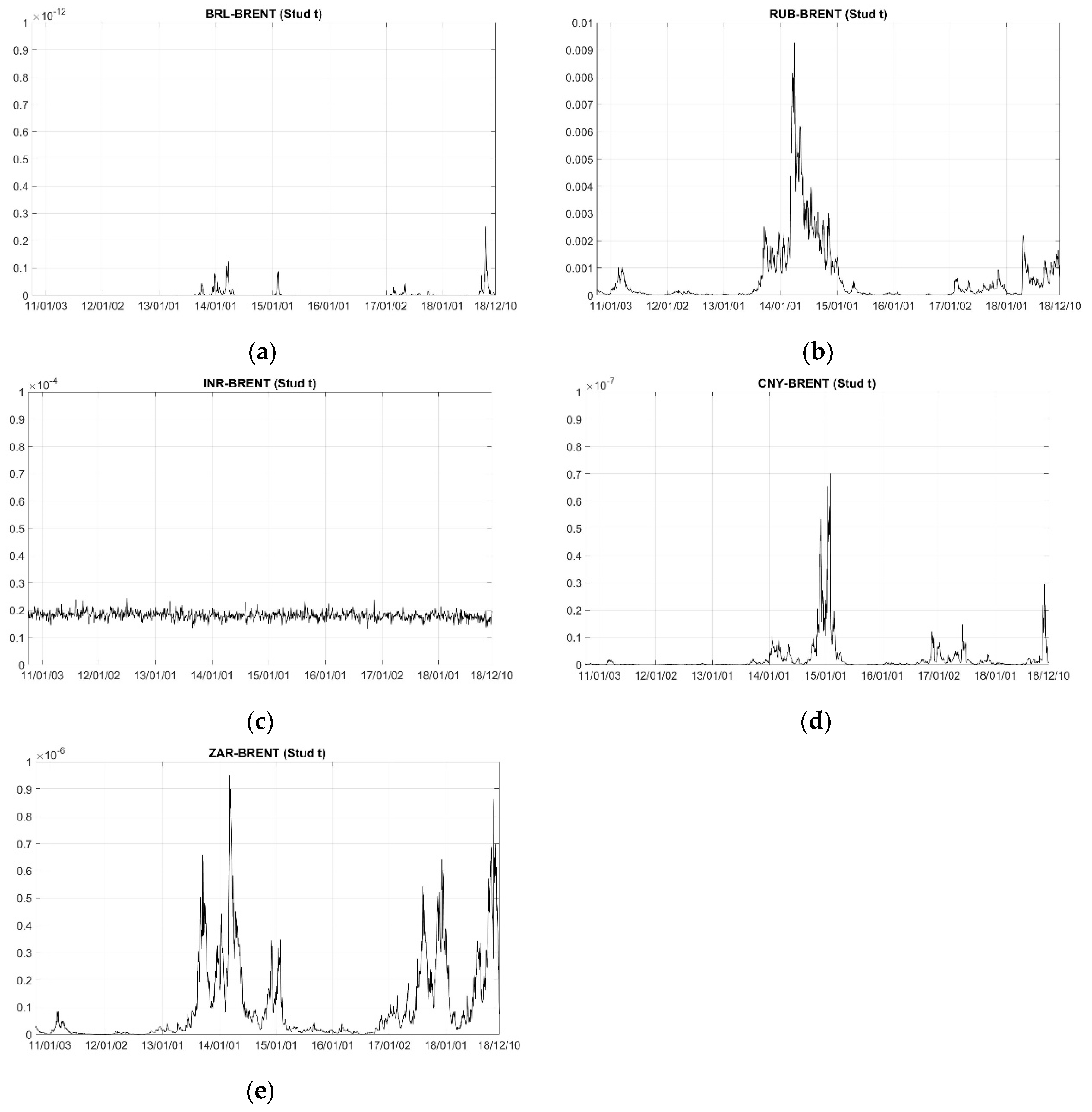
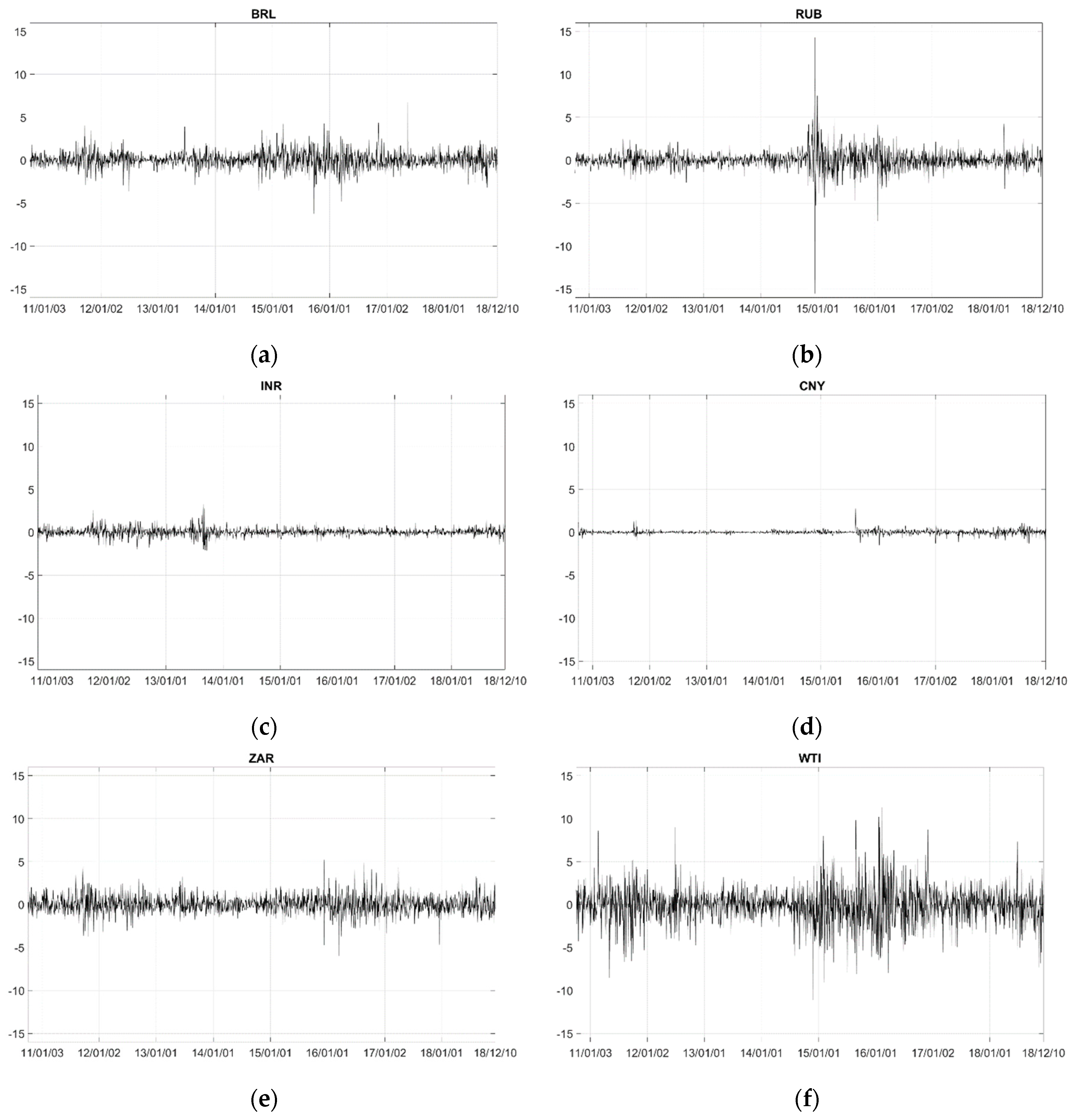
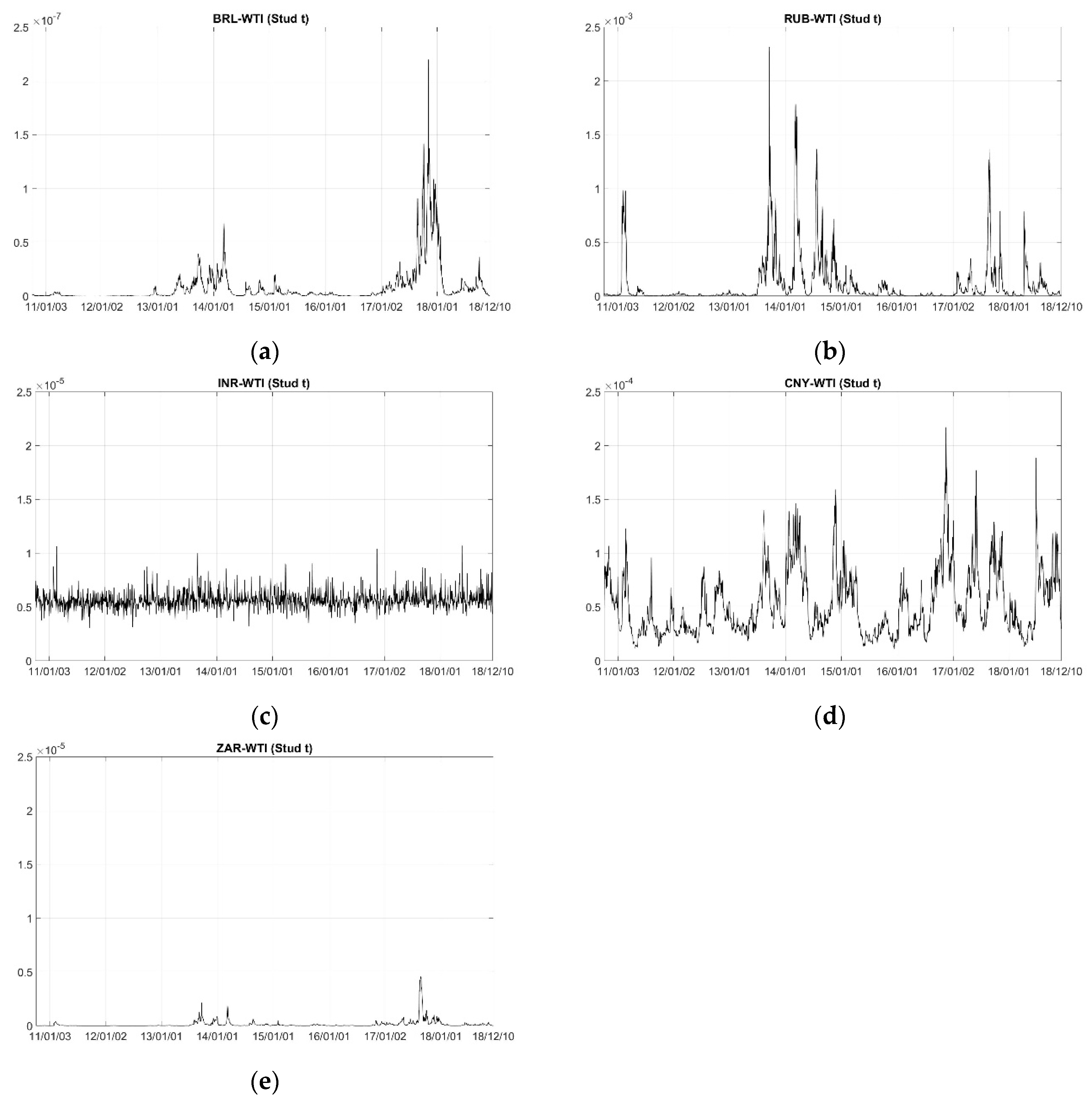
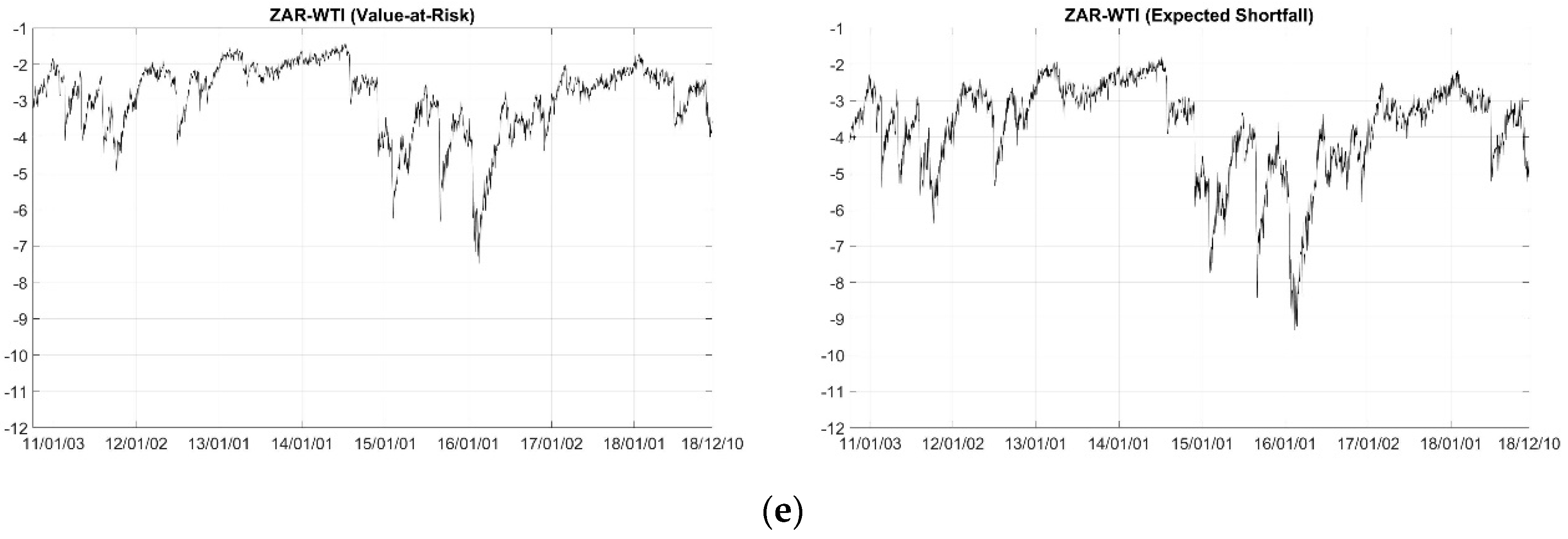
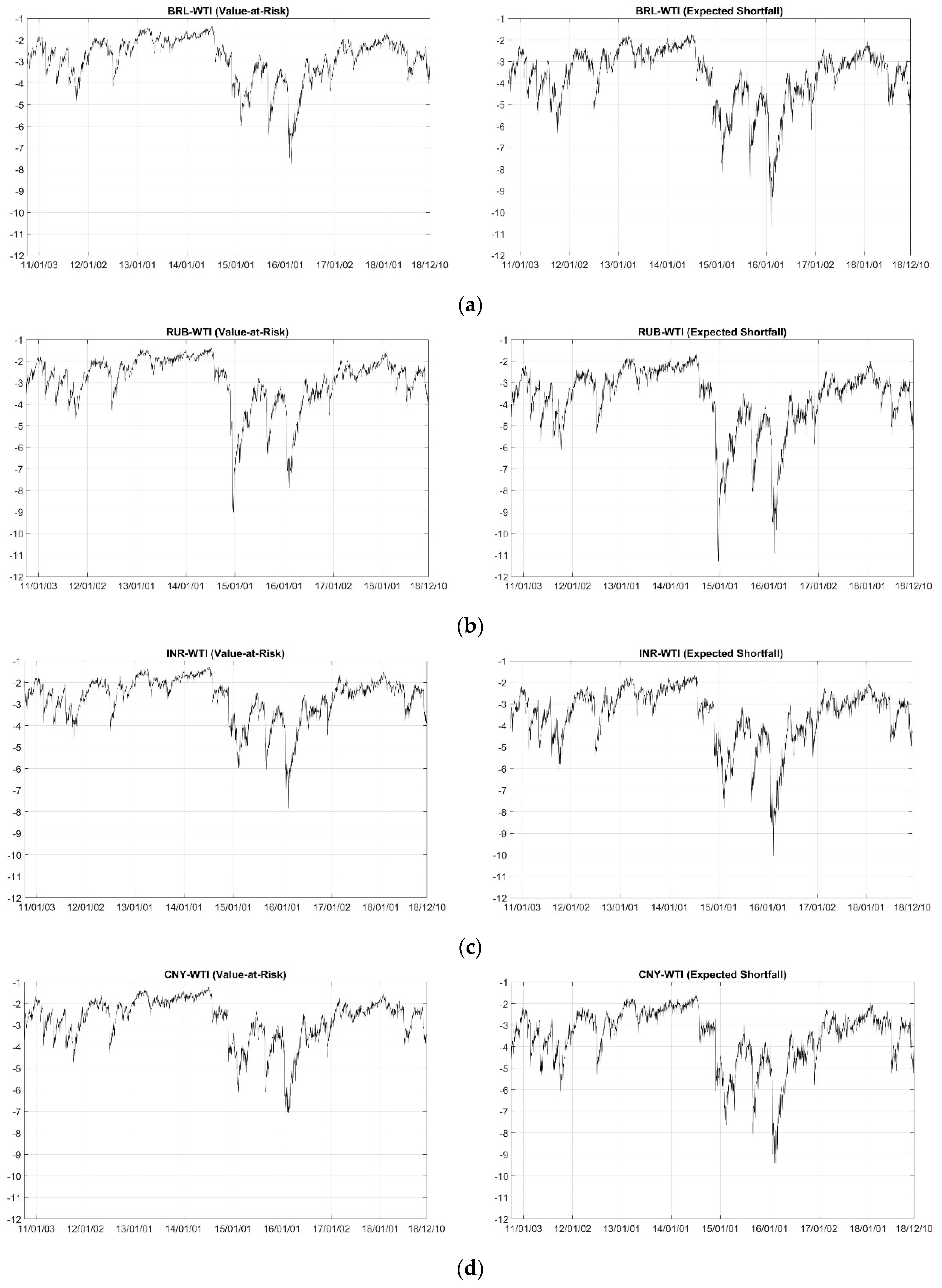
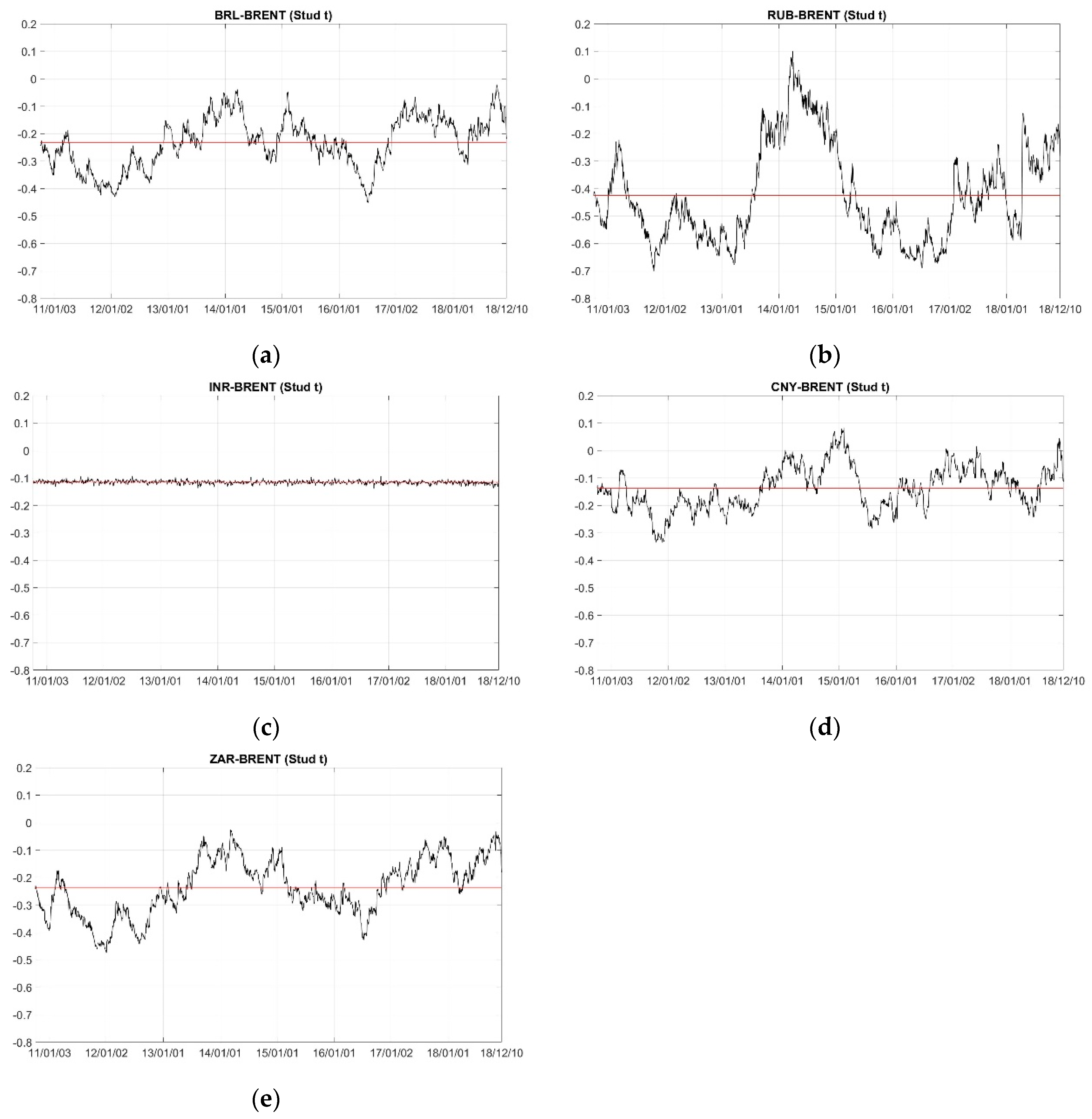
This study examined both the constant and dynamic dependencies between crude oil prices (WTI) and exchange rates for the BRICS countries, which includes oil-exporting and oil-importing economies, from 4 October 2010 to 11 December 2018. We employed constant and time-varying copula-GARCH-based models to capture the nonlinear, asymmetric, and tail dependence between the two variables.

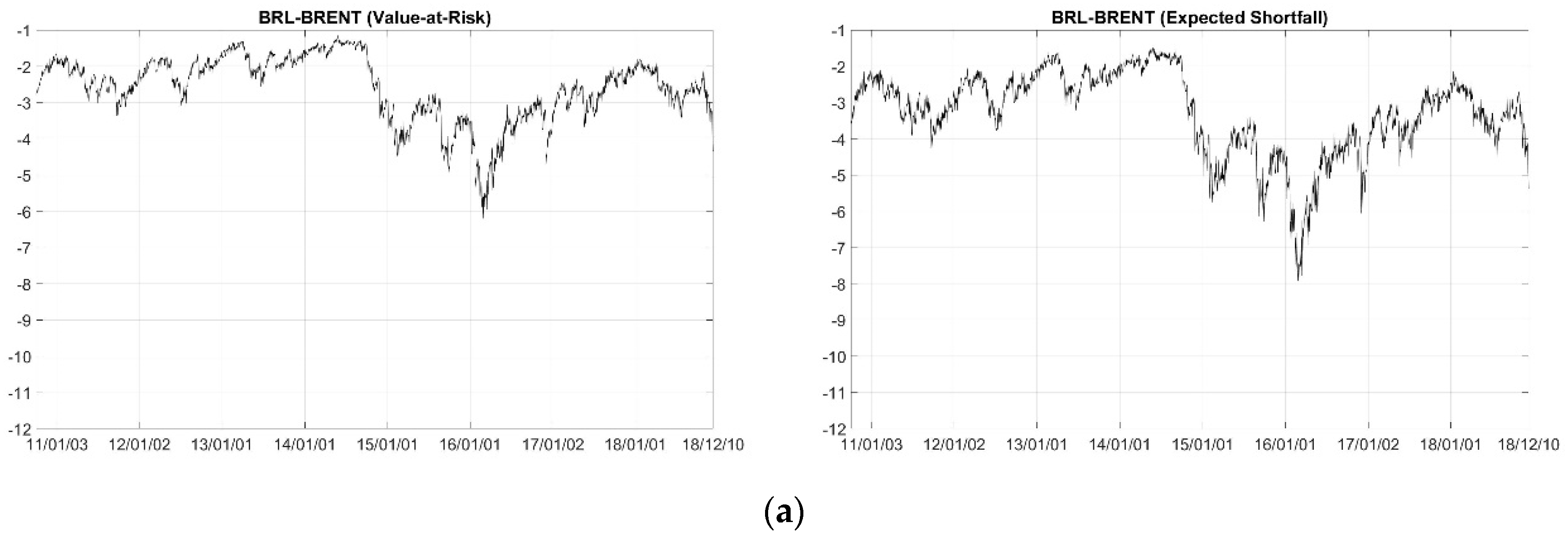
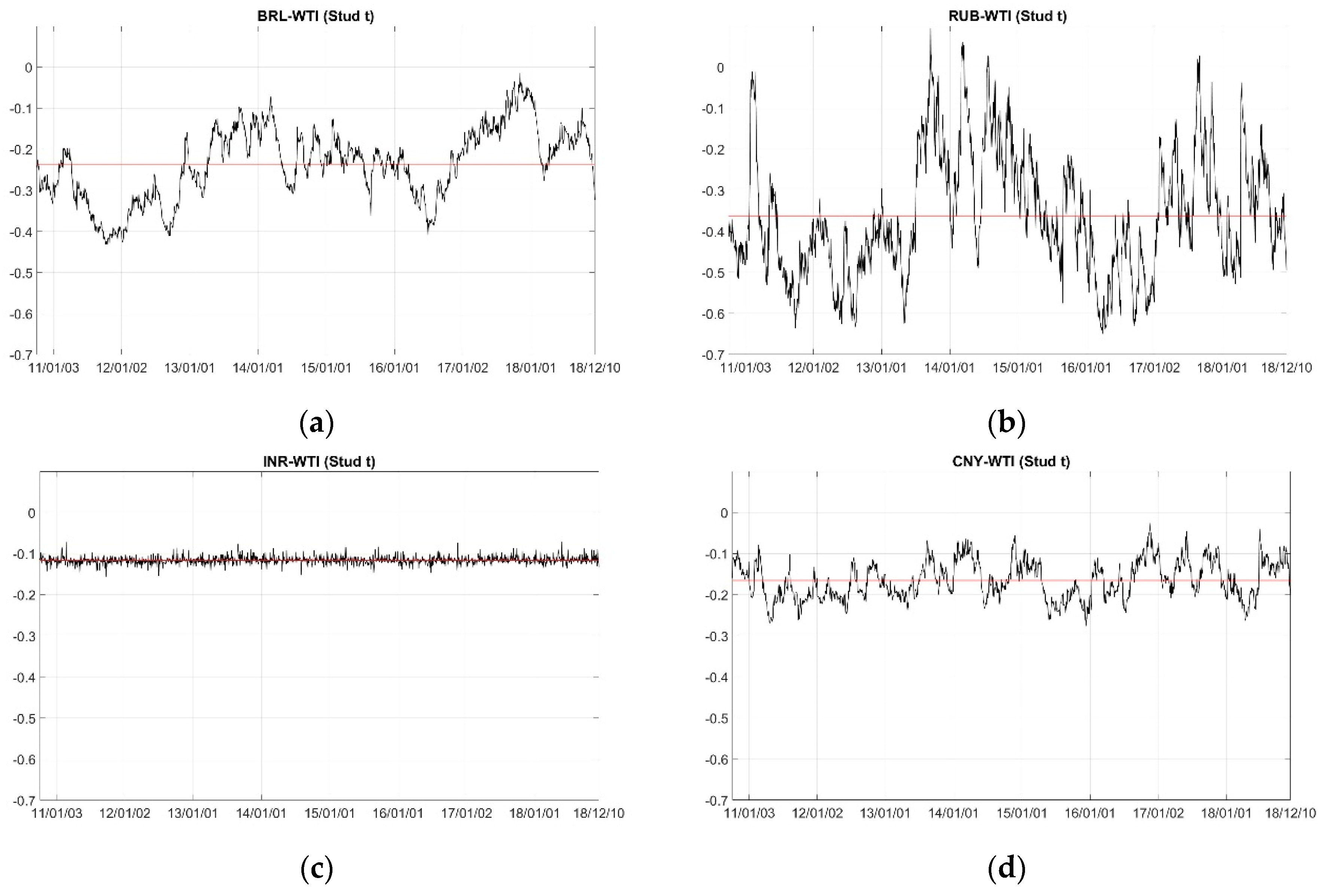
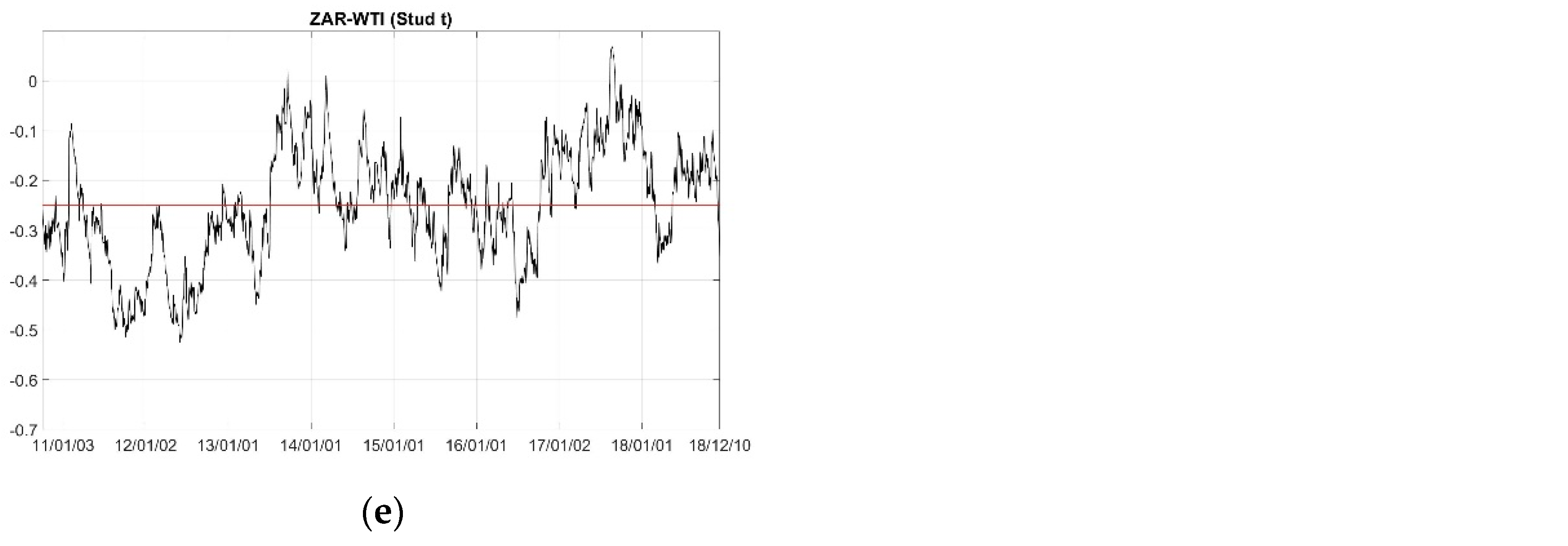
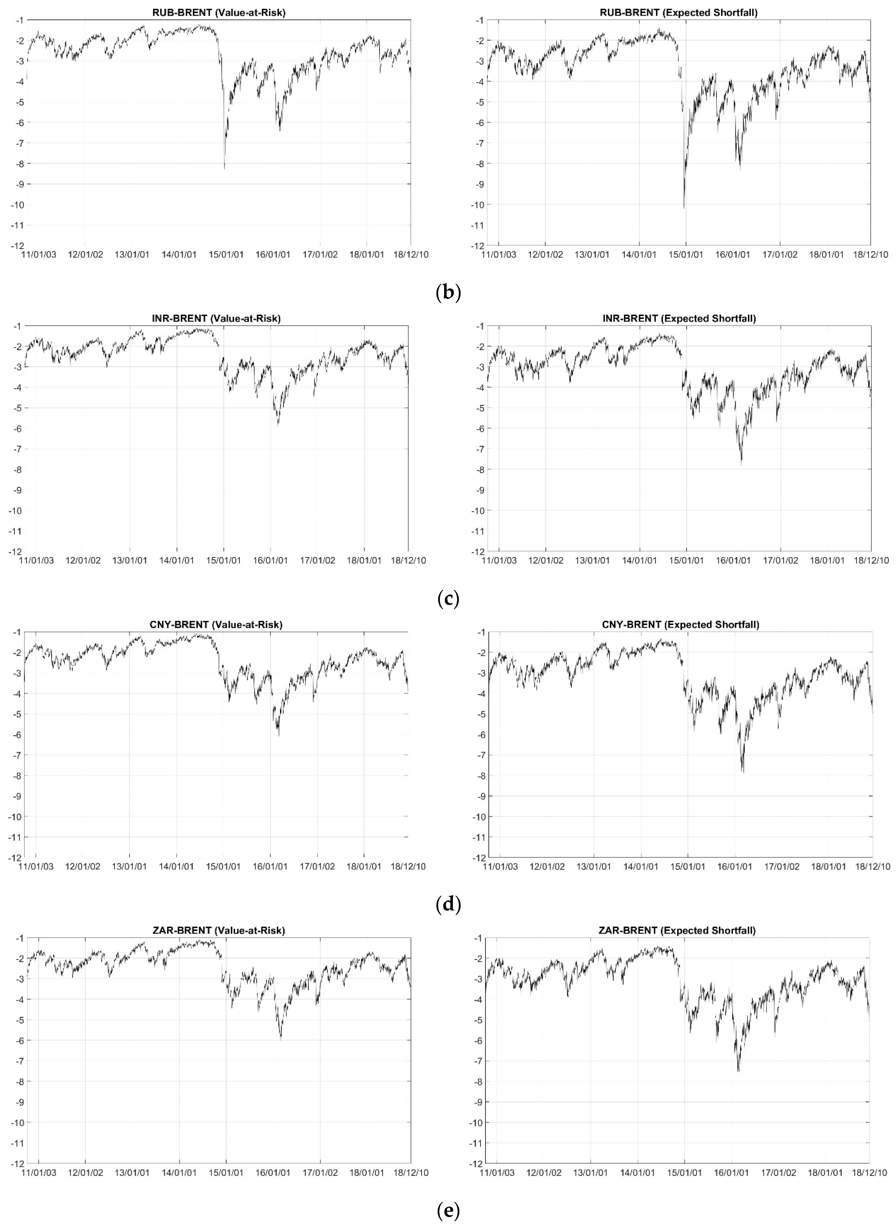
The empirical results showed, first, that a significant dependence existed in all exchange rate–oil price pairs, and the dependence is negative, which means that oil serves as a hedge against rising inflation in BRICS countries. For example, when one currency appreciates, consumers from that country will find the oil price less expensive and then increase their demand for oil, which will lead to a rise in the oil price. Second, in both the constant and time-varying copula models, the RUB–WTI pair has the strongest dependence, possibly because Russia is a large oil producer and has a high share of global oil exports, making Russia itself more dependent on oil. Third, from the goodness-of-fit test results, the Student’s t copula model has the best performance among all the constant copula models considered, while for the time-varying copula models, it was rejected for the BRL–WTI, INR–WTI, and ZAR–WTI pairs. We also measured risk management by treating the five exchange rate–oil price pairs as portfolios and calculating the dynamic values of VaR and ES. Both reached very low values for all pairs when the oil price experienced a sharp decrease.

The results of this paper offer us several suggestions. First, the significant correlation between oil price and exchange rate indicates that enterprises and governments in BRICS countries, when the oil price fluctuates, should pay attention to the exchange rate risk. Second, the negative relationship between oil price and exchange rate shows that the oil could be a hedge against inflation in BRICS countries, which is useful for foreign investors to manage exchange rate risk.

However, in this paper, we only considered bivariate copula models. For the future extension of this research, we will focus on a high-dimensional copula model, which could provide a more flexible analysis.

References

1. Akram, Q. Farooq. 2009. Commodity prices, interest rates and the dollar. Energy Economics 31: 838–51. [Google Scholar] [CrossRef]
2. Aloui, Riadh, Mohamed Safouane Ben Aïssa, and Duc Khuong Nguyen. 2013. Conditional dependence structure between oil prices and exchange rates: A copula-GARCH approach. Journal of International Money and Finance 32: 719–38. [Google Scholar] [CrossRef]
3. Bai, Jushan, and Pierre Perron. 1998. Estimating and testing linear models with multiple structural changes. Econometrica 66: 47–78. [Google Scholar] [CrossRef]
4. Bai, Jushan, and Pierre Perron. 2003. Computation and analysis of multiple structural change models. Journal of Applied Econometrics 18: 1–22. [Google Scholar] [CrossRef]
5. Basher, Syed Abul, Alfred A. Haug, and Perry Sadorsky. 2012. Oil prices, exchange rates and emerging stock markets. Energy Economics 34: 227–40. [Google Scholar] [CrossRef]
6. Beckmann, Joscha, Robert Czudaj, and Vipin Arora. 2017. The Relationship between Oil Prices and Exchange Rates: Theory and Evidence. Washington: Financial and physical Oil Market Linkages Workshop. [Google Scholar]
7. Bénassy-Quéré, Agnès, Valérie Mignon, and Alexis Penot. 2007. China and the relationship between the oil price and the dollar. Energy Policy 35: 5795–805. [Google Scholar] [CrossRef]
8. Blokhina, Tatiana K., Okasana A. Karpenko, and Andrey V. Guirinskiy. 2016. The relationship between oil prices and exchange rate in Russia. International Journal of Energy Economics and Policy 6: 721–26. [Google Scholar]
9. Bodenstein, Martin, Christopher J. Erceg, and Luca Guerrieri. 2011. Oil shock and external adjustment. Journal of International Economics 83: 168–84. [Google Scholar] [CrossRef]
10. Chen, Shiu-Sheng, and Hung-Chyn Chen. 2007. Oil prices and real exchange rates. Energy Economics 29: 390–404. [Google Scholar] [CrossRef]
11. Creal, Drew, Siem Jan Koopman, and André Lucas. 2013. Generalized autoregressive score models with applications. Journal of Applied Econometrics 28: 777–95. [Google Scholar] [CrossRef]
12. Diebold, Francis X., Jinyong Hahn, and Anthony S. Tay. 1999. Multivariate density forecast evaluation and calibration in financial risk management: High-frequency returns on foreign exchange. Review of Economics and Statistics 81: 661–73. [Google Scholar] [CrossRef]
13. Ding, Liang, and Minh Vo. 2012. Exchange rates and oil prices: A multivariate stochastic volatility analysis. The Quarterly Review of Economics and Finance 52: 15–37. [Google Scholar] [CrossRef]
14. Genest, Christian, Bruno Rémillard, and David Beaudoin. 2009. Goodness-of-fit tests for copulas: A review and a power study. Insurance: Mathematics and Economics 44: 199–213. [Google Scholar] [CrossRef]
15. Ghosh, Sajal. 2011. Examining crude oil price—Exchange rate nexus for India during the period of extreme oil price volatility. Applied Energy 88: 1886–89. [Google Scholar] [CrossRef]
16. Gisser, Micha, and Thomas H. Goodwin. 1986. Crude oil and the macroeconomy: Tests of some popular notions: Note. Journal of Monety, Credit and Banking 18: 95–103. [Google Scholar] [CrossRef]
17. Habib, Maurizio Michael, Sascha Bützer, and Livio Stracca. 2016. Global Exchange Rate Configurations: Do Oil Shocks Matter? IMF Economic Review 64: 443–70. [Google Scholar] [CrossRef]
18. Hamilton, James D. 1983. Oil and the Macroeconomy since World War II. Journal of Political Economy 91: 228–48. [Google Scholar] [CrossRef]
19. Hansen, Bruce E. 1994. Autoregressive Conditional Density Estimation. International Economic Review 35: 705–30. [Google Scholar] [CrossRef]
20. Ji, Qiang, Bing-Yue Liu, and Ying Fan. 2019. Risk dependence of CoVaR and structural change between oil prices and exchange rates: A time-varying copula model. Energy Economics 77: 80–92. [Google Scholar] [CrossRef]
21. Kin, Sibanda, and Mlambo Courage. 2014. The impact of oil prices on the exchange rate in South Africa. Journal of Economics 5: 193–99. [Google Scholar] [CrossRef]
22. Mork, Knut Anton. 1989. Oil and the macroeconomy when prices go up and down: an extension of Hamilton’s results. Journal of Political Economy 97: 740–44. [Google Scholar] [CrossRef]
23. Narayan, Seema. 2013. Foreign exchange markets and oil prices in Asia. Journal of Asian Economics 28: 41–50. [Google Scholar] [CrossRef]
24. Narayan, Paresh Kumar, Seema Narayan, and Arti Prasad. 2008. Understanding the oil price-exchange rate nexus for the Fiji Islands. Energy Economics 30: 2686–96. [Google Scholar] [CrossRef]
25. Nelsen, Roger B. 2006. An Introduction to Copulas. New York: Springer, pp. 89–121. [Google Scholar]
26. Nelson, Daniel B. 1991. Conditional Heteroskedasticity in Asset Returns: A New Approach. Econometrica 59: 347–70. [Google Scholar] [CrossRef]
27. Patton, Andrew J. 2006. Modelling asymmetric exchange rate dependence. International Economic Review 47: 527–56. [Google Scholar] [CrossRef]
28. Patton, Andrew J. 2013. Copula methods for forecasting multivariate time series. In Handbook of Economic Forecasting, 1st ed. Edited by Graham Elliott, Clive Granger and Allan Timmermann. North Holland: Elsevier, vol. 1, pp. 899–960. [Google Scholar]
29. Reboredo, Juan C., and Miguel A. Rivera-Castro. 2013. A wavelet decomposition approach to crude oil price and exchange rate dependence. Economic Modelling 32: 42–57. [Google Scholar] [CrossRef]
30. Rémillard, Bruno. 2017. Goodness-of-Fit Tests for Copulas of Multivariate Time Series. Econometrics 5: 13. [Google Scholar] [CrossRef]
31. Sklar, Abe. 1959. Fonctions de Répartition à n Dimensions et Leurs Marges. Publications de l’Institut Statistique de l’Université de Paris 8: 229–31. [Google Scholar]
32. Wu, Chih-Chiang, Huimin Chung, and Yu-Hsien Chang. 2012. The economic value of co-movement between oil price and exchange rate using copula-based GARCH models. Energy Economics 34: 270–82. [Google Scholar] [CrossRef]
1
BRICS is the acronym of an association of five major emerging economies: Brazil, Russia, India, China and South Africa.
2
For more detail, see Chen and Chen (2007).
3
EGARCH is an abbreviation for Exponential Generalized Autoregressive Conditional Heteroscedastic. EGARCH model was introduced by Nelson (1991).
4
We used Normal, Clayton, rotated-Clayton, Plackett, Frank, Gumbel, rotated-Gumbel, SJC and Student’s t copula models in our empirical analysis at first, but the log-likelihoods in the Clayton, Rotated-Clayton, Frank, Gumbel, rotated-Gumbel and SJC copulas are negative, which means that the dependence coefficients in these copula models are quiet low, so we only present the results of the Normal, Plackett, and Student’s t copula models, which have a positive log-likelihood. The rotated-Gumbel copula has the lowest log-likelihood in most currency–oil price pairs, so we also present it in the paper for comparison.
Figure 1. Daily returns on the exchange rates and crude oil prices. (af) refer to return series of BRL, RUB, INR, CNY, INR and WTI, respectively.
Jrfm 12 00099 g001
Figure 2. Dynamic parameters from the time-varying copula models. (ae) refer to BRL–WTI, RUB–WTI, INR–WTI, CNY–WTI and ZAR–WTI pairs, respectively.
Jrfm 12 00099 g002aJrfm 12 00099 g002b
Figure 3. Conditional tail dependence from the time-varying copula models. (ae) refer to pair of BRL–WTI, RUB–WTI, INR–WTI, CNY–WTI and ZAR–WTI, respectively.
Jrfm 12 00099 g003
Figure 4. Conditional 1% Value at Risk (left panel) and Expected Shortfall (right panel) for an equal-weighted portfolio based on the Student’s t copula model. (ae) refer to BRL–WTI, RUB–WTI, INR–WTI, CNY–WTI and ZAR–WTI pairs, respectively.
Jrfm 12 00099 g004aJrfm 12 00099 g004b