Clarifying the Response of Gold Return to Financial Indicators: An Empirical Comparative Analysis Using Ordinary Least Squares, Robust and Quantile Regressions

Abstract

In this study, I apply a quantile regression model to investigate how gold returns respond to changes in various financial indicators. The model quantifies the asymmetric response of gold return in the tails of the distribution based on weekly data over the past 30 years. I conducted a statistical test that allows for multiple structural changes and find that the relationship between gold return and some key financial indicators changed three times throughout the sample period. According to my empirical analysis of the whole sample period, I find that: (1) the gold return rises significantly if stock returns fall sharply; (2) it rises as the stock market volatility increases; (3) it also rises when general financial market conditions tighten; (4) gold and crude oil prices generally move toward the same direction; and (5) gold and the US dollar have an almost constant negative correlation. Looking at each sample period, (1) and (2) are remarkable in the period covering the global financial crisis (GFC), suggesting that investors divested from stocks as a risky asset. On the other hand, (3) is a phenomenon observed during the sample period after the GFC, suggesting that it reflects investors’ behavior of flight to quality.

1. Introduction

Correlations across different asset classes increased during the global financial crisis (GFC) of 2007–2009, and diversification effects did not work when most needed. With the financialization of commodities from the first half to the middle of the 2000s as cross-market linkages increased, many commodity prices plunged along with the stock market crash.1 This experience makes us recognize the importance of accurately grasping the linkages or contagion between different asset classes, and promote studies that unravel the transmission mechanism and spillover effect between different asset markets (see, e.g., Chudik and Fratzscher 2011; Diebold and Yilmaz 2012; Ehrmann et al. 2011; Guo et al. 2011; Longstaff 2010).

Gold is generally seen as distinct from other traditional assets due to its special character. It is often regarded as a safe haven, especially hedging against the downside risk of stocks or in times of financial turbulence. Academic research on gold as an investment asset has been increasing in recent years (see, for example, O’Connor et al. 2015).

Existing literature that analyze the aspects of gold as a hedge or safety instrument compared with traditional assets include Baur (2011); Baur and Lucey (2010); Baur and McDermott (2010); Cohen and Qadan (2010); Hillier et al. (2006); Hood and Malik (2013); Miyazaki et al. (2012); Miyazaki and Hamori (2013, 2014, 2016, 2018); Piplack and Straetmans (2010); Qadan and Yagil (2012); World Gold Council (2010).

Baur (2011) analyzes the characteristics of gold based on multiple regression. He finds that gold has a hedging function against US dollar depreciation but not against inflation as represented by consumer prices. In addition, he argues that the role of gold as a safety asset is a phenomenon seen more recently. Piplack and Straetmans (2010) examined the tail dependence between US stocks, government bonds, Treasury bills, and gold using the extreme value theory, and conducted statistical tests for flight to quality or flight to liquidity hypotheses. Their empirical results show that gold is, to some extent, effective as a safe asset against the plunge in the values of other assets. Furthermore, there are many existing studies that analyze the properties of commodities including gold as an investment vehicle (e.g., Akram 2009; Batten et al. 2010, 2014; Bhar and Hammoudeh 2011; Chan et al. 2011; Chevallier and Ielpo 2013; Ciner et al. 2013; Erb and Harvey 2006; Gorton and Rouwenhorst 2006; Hammoudeh et al. 2009; Mensi et al. 2013; Sari et al. 2010; Silvennoinen and Thorp 2013, among others). In addition to these studies, Alkhatib and Harasheh (2018); Balcilar et al. (2018); Raza et al. (2018) covers up to more recent sample period during and after the Brexit.

In this study, I use robust and quantile regression techniques to investigate how gold return responds to the changes in various financial indicators, specifically stock return, stock return volatility, financial market stress, crude oil, and the value of the US dollar. In the finance literature involving empirical analyses, there are also many cases where interest is on the tails of the distribution rather than the average (expected value). Quantile regression introduced by Koenker and Bassett (1978) allows us to clarify the relationships between dependent variables and independent variables in the tails of the distributions of data that cannot be captured by only the expected value. Therefore, in recent years in the field of economics and finance, econometricians have come to frequently use quantile regression making it one of the standard tools. Quantile regression is suitable for the purpose of this study in quantifying the role of gold as a hedging function or safety asset.2 Empirical research using quantile regression include Baur (2013); Baur and Schulze (2005); Bouoiyour et al. (2018); Mensi et al. (2014); Reboredo and Uddin (2016); Reboredo and Uddin (2016) applied quantile regression to analyze the impact of financial stress and policy uncertainty in the US on a wide range of commodity futures prices.

This paper clarifies the role or characteristics of gold as an investment asset, on which, so far, academic research has been relatively scarce in the finance literature. Similar to the motivation of Reboredo and Uddin (2016), this study is also interested in the way gold return responds to a surge in financial market stress, sharp drop in stock prices, and stock market volatility. One novelty of this study is that it considers multiple structural breaks that are endogenously determined. Our empirical results show that the relationship between gold and financial variables mentioned above is not stable and have experienced several structural changes over time. In addition, we provide evidence that gold return rises in response to a plunge in stock prices and a rapid rise in stress in the financial markets, suggesting the role of gold as a safe haven. This result tells us that investors are taking a “flight-to-quality” behavior.

The rest of the paper is organized as follows. In the next section, we briefly outline econometric methodologies used in this paper comprising robust and quantile regression techniques. In addition to presenting data for the analysis, we construct the indicators to measure the level of stress in the financial markets in Section 3. Section 4 presents our major empirical results, while Section 5 concludes.

2. Econometric Methodology

In this section, we outline the robust and quantile regression techniques to be used in this study. While both regression techniques address outliers in the data and asymmetry of distributions, their concepts and approaches are considerably different.

2.1. Robust Regression

The property of an ordinary least squares (OLS) estimator being BLUE (Best Linear Unbiased Estimator) depends on the assumption about the error term. Robust regression is an estimation method for correcting the bias of the OLS estimator caused by the existence of outliers and heteroskedasticity. OLS places equal weights to all observations, whereas robust regression reduces the weights on outliers to mitigate the latter’s influence. Robust regression is insensitive to small changes in the sample and distributional assumptions of the data. It is also useful in separating the contribution of the part of the data near the average and the part in the tails.3

Among the different variations of weight functions, I choose Bisquare defined as follows.

$$\{\begin{array}{cc}\frac{c^2}{6}\left(1-{\left(1-{\left(\frac{X}{c}\right)}^2\right)}^3\right),& \mathrm{if} \left|X\right|\le c,\\ \frac{c^2}{6},& \mathrm{otherwise},\end{array}$$

(1)

where $c$ is an arbitrary positive tuning constant set to $c=4.685$ in Bisquare form.4

2.2. Quantile Regression

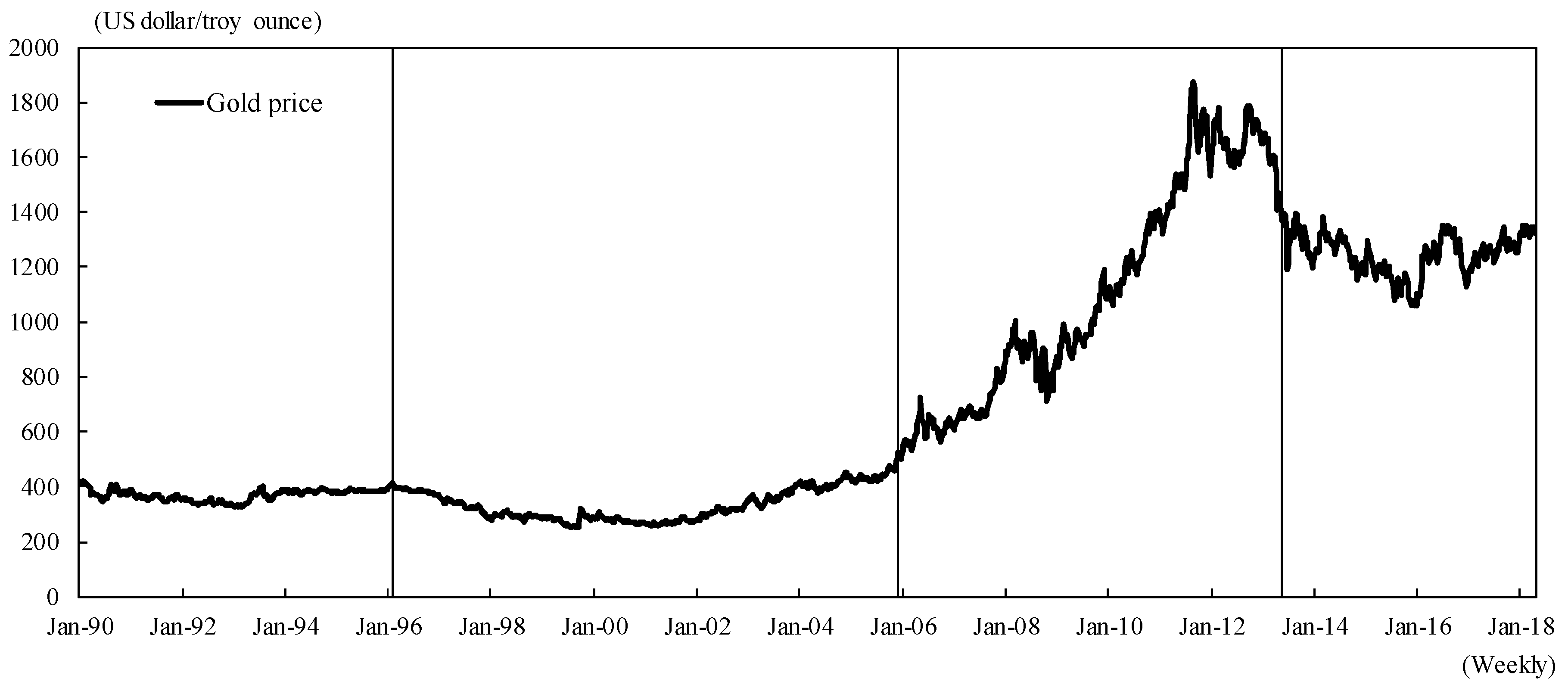
Quantile regression is a method of modeling and estimating the relationship between a dependent variable and independent variables in the tails of the distribution (more specifically, quantile).5 The distribution of returns of financial assets frequently exhibits the statistical property of heavy tails (see, for example, Cont 2001). If heavy tails and/or asymmetry in the distributions exist, the assumption of normality is not satisfied. Therefore, inference based on classical regression models may lead to misleading conclusions. By utilizing quantile regression, researchers can reveal more accurate dependence structure between variables according to market conditions such as bull or bear markets, and completely know the distribution of returns.

OLS minimizes the sum of squared residuals,

$$\underset{\alpha ,\beta }{\min }{\displaystyle \sum }_{t=1}^T{\left(y_t-\alpha -\beta x_t\right)}^2$$

(2)

whereas quantile regression minimizes the following loss function,

$$\underset{\alpha \left(\tau \right),\beta \left(\tau \right)}{\min }{\displaystyle \sum }_{t=1}^T{\rho }_{\tau }\left(y_t-\alpha \left(\tau \right)-\beta \left(\tau \right)x_t\right)$$

(3)

where ${\rho }_{\tau }\left(u\right)$ is the check function defined as follows.

$${\rho }_{\tau }\left(u\right)=u\left(\tau -1\left\{u\le 0\right\}\right)=\{\begin{array}{cc}-\left(1-\tau \right)u,& u\le 0\\ \tau u,& u>0\end{array}$$

(4)

where $u=y_t-\alpha \left(\tau \right)-\beta \left(\tau \right)x_t$, and $\tau \in \left(0, 1\right)$ indicates the level of quantile. In particular, if $\tau =0.5$, that is the median, the quantile regression corresponds to the least absolute deviation method.

In summary, the techniques of robust regression and quantile regression model and estimate the relationships between the dependent variable and independent variables in the center of and in the tails of data distribution, respectively. Resorting to these two regression methods, we can closely shed light on the characteristics of gold return than in previous literature.

3. Data

We adopt the US as a reference market affecting gold price. The US still possesses a dominant influence in the global financial markets, and plays the most important role to transmit financial shocks (see, e.g., Chudik and Fratzscher 2011; Ehrmann et al. 2011). In this study, we focus on the relationships between gold and a variety of financial indicators, specifically stock market return, stock market return volatility, crude oil, the value of the US dollar against major currencies, and general financial market conditions in the US.6 The sample period covers about past three decades of weekly data from 5 January 1990 to 27 April 2018. Weekly frequency seems to be an appropriate choice to ensure the number of samples and eliminate noise that can occur in daily data.

Table 1. Data sources.

Variable	Source
Gold price, PM fix (spot)	Bloomberg; originally provided by London Bullion Market Association (LBMA)
S&P 500 Index (spot)	Bloomberg; originally provided by S&P Dow Jones Indices
TED spread	Federal Reserve Economic Database (FRED) of St. Louis Fed
Aaa-10Y spread	Federal Reserve Economic Database (FRED) of St. Louis Fed
Baa-Aaa spread	Federal Reserve Economic Database (FRED) of St. Louis Fed
West Texas Intermediate (WTI) (spot)	Federal Reserve Economic Database (FRED) of St. Louis Fed; originally provided by US Energy Information Administration (EIA)
Trade Weighted US Dollar Index: Major Currencies	Federal Reserve Economic Database (FRED) of St. Louis Fed; originally provided by Board of Governors of the Federal Reserve System (US)

displays the data sources. All three financial instruments, namely gold, S&P 500 index and crude oil are spot prices.

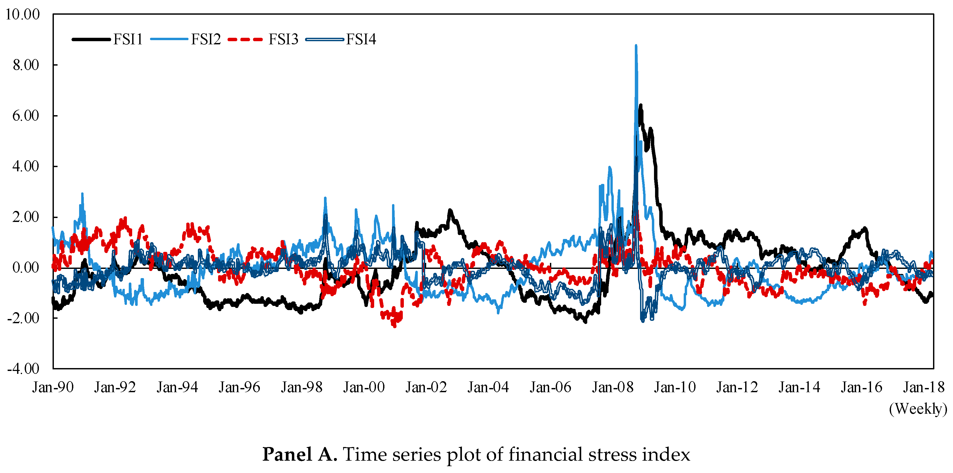
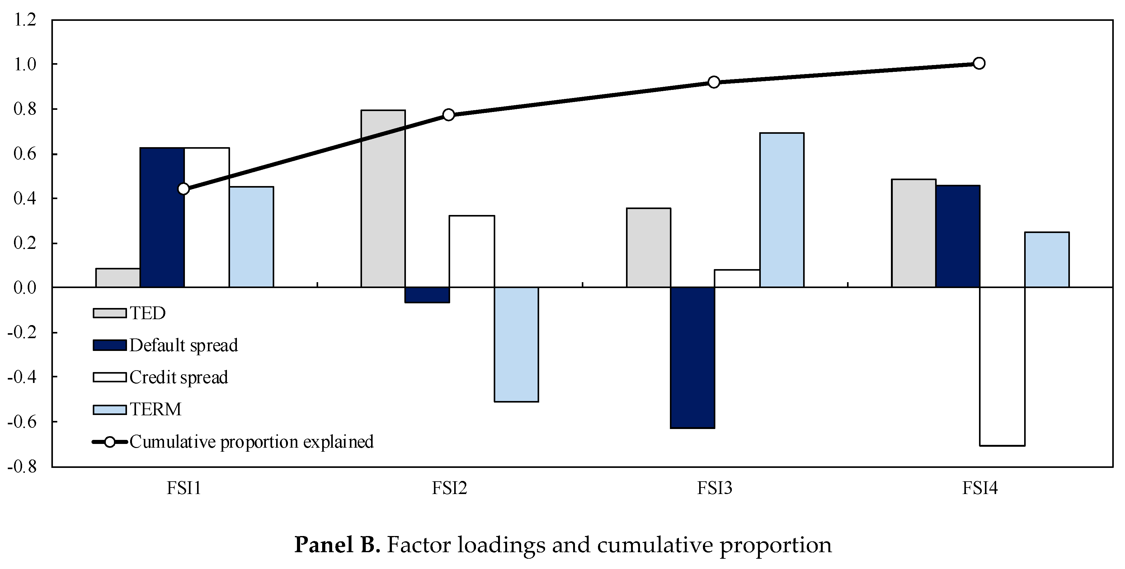
3.1. Measure of Financial Market Stress

Several variables could serve as indicators of financial market conditions. To construct an index to measure the stress level of financial markets, we employ principal component analysis (PCA). Specifically, we apply PCA to the following four interest rate-related variables; Treasury-EuroDollar (TED) spread,7 credit spread,8 default spread,9 and term spread,10 and set the extracted principal components as a measure for the degree of financial market stress.11 These financial indicators act as liquidity risk, credit risk, default risk, and monetary policy stance or recession risk,12 respectively.

Table 2. Principal component analysis: financial market stress.

	Factor Loadings
	1st	2nd	3rd	4th
TED	0.088	0.796	0.354	0.483
Aaa-10Y	0.628	−0.068	−0.626	0.458
Baa-Aaa	0.627	0.324	0.079	−0.704
TERM	0.453	−0.507	0.690	0.247
% variance explained	44.18	33.01	14.56	8.26

Notes: This table summarizes the results of the principal component analysis applied to a set of financial risk indicators (TED, Aaa-10Y, Baa-Aaa, and TERM). TED is the spread between the three-month London interbank offered rate based on the US dollars and the three-month Treasury bill rate. Aaa-10Y is the yield spread between Aaa-ranked corporate bonds and Treasuries with 10-year constant maturities. Baa-Aaa is the yield spread between Baa- and Aaa-ranked corporate bonds. TERM is the yield spread between Treasuries of 10-year and three-month constant maturities.

reports the results of PCA extracted from the four risk indicators above, and Figure 1 illustrates their evolution. According to Table 2, factor loadings of all financial risk indicators are positive for the first principal component. As seen in Figure 1, the first principal component experiences spikes in the financial turmoil episodes such as failure of long-term capital management (LTCM), dot-com bubble collapse, and Lehman Brothers bankruptcy. From these observational findings, we interpret the first principal component as the degree of general financial market stress and use it as an indicator to measure the tightness of the financial market in the following empirical analysis.

3.2. Summary Statistics

The purpose of this study is to examine empirical dependence structure between gold and key financial indicators. We take up five financial indicators considered affecting gold return, namely stock return, stock market volatility, financial market stress, crude oil, and the value of the US dollar. Risk-averse investors demand gold as a hedge against the downside risks of stock market. Gold generally has a low correlation with traditional assets such as stocks and offers an option for an effective diversification investment (World Gold Council 2010). We use S&P 500 Index return and its volatility as a variable representing the stock market conditions. Furthermore, investors demand gold as a safe haven in times of financial turmoil. This phenomenon is an investor behavior generally called “flight to quality.” A variable representing the tightness of financial markets is the financial market stress index constructed above. We choose crude oil as a representative commodity belonging to the same asset class as gold, and specifically use the West Texas Intermediate (WTI). Gold is known to be inversely associated with the US dollar since gold functions as a store of value or loss compensation against depreciations in the US dollar (see, for example, Miyazaki and Hamori 2016). We use the trade-weighted US dollar exchange rate as a variable representing the value of the US dollar.

For gold, S&P 500 Index, WTI, and trade-weighted US dollar exchange rate, we transform the series by log-differencing. As for the stock return volatility, we use the square root of the estimates obtained by applying an exponential generalized autoregressive conditional heteroskedasticity (EGARCH) model to the S&P 500 Index return13. Because crude oil and gold are priced in dollars, fluctuations in the US dollar rate serve as a common factor in the price fluctuations of both commodities (Sari et al. 2010). To eliminate the effect of this common factor in the following empirical analysis, we use as WTI the residuals obtained by regressing WTI on the value of US dollar.

Panels A and B of

Table 3. Summary statistics.

Panel A: Descriptive Statistics
	GOLD	SPX	SPVOL	FSI1	WTI	TWEX
Mean	0.080	0.137	2.048	0.001	0.000	−0.003
Maximum	14.694	11.356	9.885	6.426	25.114	4.342
Minimum	−13.790	−20.084	0.862	−2.136	−18.972	−3.851
Std. Dev.	2.227	2.256	0.867	1.330	4.182	0.946
Skewness	−0.133	−0.753	2.547	1.406	−0.128	0.180
Kurtosis	7.543	9.853	15.000	6.921	6.035	4.064
Jarque–Bera	1274.215	3029.719	10,459.200	1432.904	571.023	77.579
p-value	0.000	0.000	0.000	0.000	0.000	0.000
Num. of obs.	1477	1477	1477	1477	1477	1477
Panel B: Correlation Matrix
	GOLD	SPX	SPVOL	FSI1	WTI	TWEX
GOLD	1.000
SPX	−0.039	1.000
SPVOL	−0.032	0.029	1.000
FSI1	0.028	−0.051	0.550	1.000
WTI	0.113	0.076	−0.077	−0.055	1.000
TWEX	−0.394	−0.134	0.013	−0.005	0.000	1.000

Notes: Data is weekly frequency. The sample period spans from 12 January 1990, to 27 April 2018. In Panel A, the p-value is the probability that corresponds to the Jarque–Bera test of normality. GOLD denotes the log-differenced gold return. SPX denotes the log-differenced return for the S&P 500 Index. SPVOL denotes the S&P 500 Index return volatility. FSI1 the degree of financial market stress (the first principal component extracted from PCA). WTI denotes the return on West Texas Intermediate (the residual obtained from regressing WTI on TWEX). TWEX denotes the appreciation/depreciation rate of the US dollar against major currencies.

report the descriptive statistics and the correlation matrix of variables used in following empirical analysis. The mean of returns on gold and S&P 500 Index is 0.080 and 0.137, respectively. Since the WTI returns are the residuals regressed to the trade-weighted US dollar exchange rate, its mean is zero. Fluctuations in returns on gold and S&P 500 Index from the standpoint of standard deviation are on the same magnitude, and the return on WTI shows the largest fluctuation. The returns on gold, S&P 500 Index and WTI have negative skewness. Thus, these variables have a heavy left tail in the distribution, meaning they occasionally show a large negative return. Contrarily, the S&P 500 Index return volatility, the financial market stress index, and the trade-weighted US dollar exchange rate have positive skewness. Thus, these variables have a heavy right tail in the distribution, meaning they occasionally show a sharp rise. For all of the time series, kurtosis exceeds three, indicating these variables are leptokurtic. As shown in the Jarque–Bera test statistics and the corresponding p-values, the null hypothesis of normality is strongly rejected for all of time series.

As can be seen in Panel B of Table 3, gold return is weakly negatively correlated with the two variables of the US stock market and is positively correlated with financial market stress and WTI. As expected, gold return has a moderate negative correlation with the US dollar. Not surprisingly, financial market stress and stock market volatility show a positive correlation, suggesting a widespread financial turmoil is likely to be accompanied by a volatile stock market. Somewhat oddly, although it seems that market volatility tends to increase when the stock market declines, the S&P 500 Index return and its volatility show a weak positive correlation. As a matter of course, the correlation coefficient, however, can only capture a symmetric linear relationship between variables.

4. Empirical Results

4.1. OLS and Robust Regression Results

Although the fundamental price of gold is sometimes derived from a convenience yield using futures prices, there is no theoretical model accepted widely like the discounted present value model for stocks. Our model estimated below, therefore, is entirely an empirical model.

The regression equation we estimate is given by,14

$$\begin{gathered} GOL{D}_t={\beta }_0+{\displaystyle \sum }_{i=1}^5{\beta }_{i}GOL{D}_{t-i}+{\beta }_{6}SP{X}_t+{\beta }_{7}SPVO{L}_t+{\beta }_{8}FSI{1}_t+{\beta }_{9}WT{I}_t \\ +{\beta }_{10}TWE{X}_t+e_t \end{gathered}$$

(5)

where $GOLD$ is gold return, $SPX$ is S&P 500 Index return, $SPVOL$ is S&P 500 Index return volatility, $FSI1$ is the degree of financial market stress (the first principal component extracted from PCA in the previous section), $WTI$ is return on West Texas Intermediate (the residual obtained from regressing $WTI$ on $TWEX$), $TWEX$ is the appreciation/depreciation rate of the US dollar, ${\beta }_j$ ($j=0,\cdots ,10)$ is the parameters to be estimated, and $e$ is the error term.

Before turning to the estimation of the model, we implement a test for structural change developed by Bai and Perron (1998, 2003a, 2003b), which enables us to identify multiple breakpoints. In their test, the number of structural changes considered increases sequentially. Firstly, I test the alternative hypothesis that “the number of structural changes is one” against the null hypothesis of “no structural change.” Secondly, If the null hypothesis is rejected, we next test the alternative hypothesis that “the number of structural changes is two” against the null hypothesis that “the number of structural changes is one.” More generally, the null hypothesis can be written as “the number of structural changes is $m$ times,” and the alternative hypothesis as “the number of structural changes is $m+1$ times.” This procedure is continued until the null hypothesis is accepted. As a result of Bai and Perron’s (1998, 2003a, 2003b) test, we identified three breakpoints, namely, 2 February 1996, 2 December 2005, and 10 May 2013 (see

Table 4. Multiple breakpoint test.

H0	H1	Test Statistic	Critical Value	Breakpoint
No break	1 time break	75.49 **	27.03	2/02/1996
1 time break	2 times break	52.16 **	29.24	12/02/2005
2 times break	3 times break	50.21 **	30.45	5/10/2013
3 times break	4 times break	12.92	31.45

Notes: ** denotes statistical significance at the 5% and 1% levels.

). Thus, the whole sample period is divided into four subsample periods.15

Figure 2 depicts the behavior of gold price together with the structural breakpoints (break dates are exhibited by solid vertical lines). What kind of economic reasons can be given as a background to the structural breakpoints identified in these periods? A possible explanation for the first structural break date is an adoption of “strong dollar policy” led by Robert Rubin, United States Secretary of the Treasury. Gold prices are closely linked to changes in the value of the US dollar. With this policy, US dollar appreciated and the gold price declined. The second structural breakpoint is connected with the development of financialization of commodities. This trend promoted to strengthen the correlation among various asset classes as mentioned in Introduction. Among the three structural breaks, the second break date, 2 December 2005, approximately coincides with the one found by Miyazaki and Hamori (2014).16 The last structural breakpoint can be attributed to the emergence of anticipation that the loosening monetary policy in the US, specifically Quantitative Easing program 3, implemented after the GFC, is going to shrink. This anticipation has caused an appreciation of the US dollar, and has led gold prices, which has been boomed since the GFC, turned to fall.

Table 5. OLS and robust regression results.

Dependent Variable: GOLD
	A. Full Sample: 2/16/1990–4/27/2018				B. First Sample: 2/16/1990–1/26/1996				C. Second Sample: 2/02/1996–11/25/2005
	Number of Observations: 1472				Number of Observations: 311				Number of Observations: 513
	OLS		Robust regression		OLS		Robust regression		OLS		Robust regression
	Coefficient	S.E.	Coefficient	S.E.	Coefficient	S.E.	Coefficient	S.E.	Coefficient	S.E.	Coefficient	S.E.
SPX	−0.099 **	0.036	−0.055 **	0.020	−0.228 **	0.045	−0.182 **	0.047	0.004	0.028	−0.011	0.026
SPVOL	−0.101	0.111	−0.099	0.063	−0.367 *	0.165	−0.672 **	0.146	−0.115	0.099	−0.183 *	0.093
FSI1	0.096	0.058	0.078	0.041	0.145	0.120	0.160	0.113	0.148	0.076	0.201 **	0.066
WTI	0.065 **	0.015	0.046 **	0.011	0.090 **	0.019	0.083 **	0.018	0.015	0.016	0.018	0.014
TWEX	−0.962 **	0.082	−0.892 **	0.048	−0.155	0.105	−0.151	0.079	−0.850 **	0.091	−0.870 **	0.070
Constant	0.312	0.231	0.302 *	0.136	0.744 *	0.324	1.240 **	0.265	0.344	0.227	0.460 *	0.226
Adj R2		0.186		0.263		0.126		0.232		0.200		0.338
	Breusch–Pagan–Godfrey test				Breusch–Pagan–Godfrey test				Breusch–Pagan–Godfrey test
	${\chi }^2\left(10\right)$			0.000	${\chi }^2\left(10\right)$			0.136	${\chi }^2\left(10\right)$			0.001
	White test				White test				White test
	${\chi }^2\left(65\right)$			0.000	${\chi }^2\left(65\right)$			0.000	${\chi }^2\left(65\right)$			0.006
	D. Third sample: 12/02/2005–5/03/2013				E. Fourth sample: 5/10/2013–4/27/2018
	Number of observations: 388				Number of observations: 260
	OLS	Robust regression	OLS	Robust regression
	Coefficient	S.E.	Coefficient	S.E.	Coefficient	S.E.	Coefficient	S.E.
SPX	−0.267 **	0.078	−0.177 **	0.049	−0.126	0.069	−0.095	0.065
SPVOL	−0.063	0.249	0.157	0.149	0.222	0.163	0.092	0.210
FSI1	0.045	0.127	−0.109	0.092	−0.062	0.139	−0.049	0.164
WTI	0.154 **	0.032	0.129 **	0.030	−0.052	0.027	−0.046	0.029
TWEX	−1.573 **	0.182	−1.513 **	0.129	−1.131 **	0.130	−1.102 **	0.117
Constant	0.437	0.513	0.060	0.322	−0.329	0.297	−0.116	0.361
Adj R2		0.316		0.401		0.299		0.381
	Breusch–Pagan–Godfrey test				Breusch–Pagan–Godfrey test
	${\chi }^2\left(10\right)$			0.000	${\chi }^2\left(10\right)$			0.007
	White test				White test
	${\chi }^2\left(65\right)$			0.000	${\chi }^2\left(65\right)$			0.181

Notes: S.E. stands for standard error. For the OLS regression, the standard errors are adjusted by using the Newey–West (1987) method. Adj R² for robust regression shows adjusted R²_W proposed by Renaud and Victoria-Feser (2010). * and ** denote statistical significance at the 5% and 1% levels, respectively.

summarizes the estimation results based on OLS and robust regression. The OLS and robust regression results are roughly similar. In the full sample period, the results of the significance test for coefficients are the same except for the constant term. In both OLS and robust regression, gold return has a negative correlation with the S&P 500 Index return, but in the robust regression the estimate drops to about half of OLS. Thus, it seems that the estimate by OLS has a bias caused by outliers. In fact, turning to the results of the two tests (Breusch–Pagan–Godfrey and White) for heteroskedasticity reported at the bottom of panel A in Table 5, the null hypothesis of no heteroskedasticity is strongly rejected. Therefore, the robust regression provides us with more reliable results than those of the OLS. The gold return is positively associated with crude oil return. This relation indicates that both prices tend to move toward the same direction, suggesting that investors perhaps regard these two commodities as belonging to the same asset class. The coefficient for the value of US dollar is close to one in absolute terms, indicating that gold return moves nearly in a one-to-one negative correlation with the value of the US dollar.

Then, we turn to the results of each subsample period. In the first sample, besides the returns on the S&P 500 Index and WTI, the stock return volatility is estimated significantly. However, its sign is negative and is opposite to the expected sign, whereas a significant relationship with the US dollar has disappeared. Breusch–Pagan–Godfrey and White tests present mixed evidence for heteroskedasticity, that is, the former cannot reject homoskedasticity hypothesis, while the latter reject the hypothesis. Therefore, we cannot clearly determine which of the OLS and robust regression results are reliable. In any case, however, estimated coefficients do not differ greatly in magnitude.

The second sample period has the largest number of observations among the four subsamples, and the OLS and robust regression results show some differences. In the OLS estimation, only the US dollar is significant, while in robust regression, stock return volatility is still negative and significant, and the rise in financial market stress works to push the gold return up significantly. The latter is consistent with the expected sign. Both of two tests for heteroskedasticity reject the null hypothesis, suggesting that employing robust regression is adequate.

In the third and fourth subsamples, we find no noticeable difference when comparing both estimation results. Although the results of the third sample period are similar to the those of the full sample, the coefficients for the stock return, WTI, and US dollar are approximately two or three times larger than those in the full sample. This finding implies that the connection between gold and the financial variables has strengthened during this period, consistent with the financialization of commodities. Both of two tests for heteroskedasticity reject the null hypothesis, indicating that resorting to robust regression is suitable.

For the fourth sample period, only the coefficient on the US dollar is negative and significant. Two tests for heteroskedasticity lead us to different conclusions, respectively, similar to the first sample period. Although neither is significant, there are some differences in estimated coefficient of S&P 500 Index volatility and constant term, between two methods.

In the following subsection, we present the results using quantile regression to explore the relationship in the tails of the distribution that cannot be captured by OLS and robust regressions.

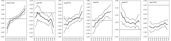
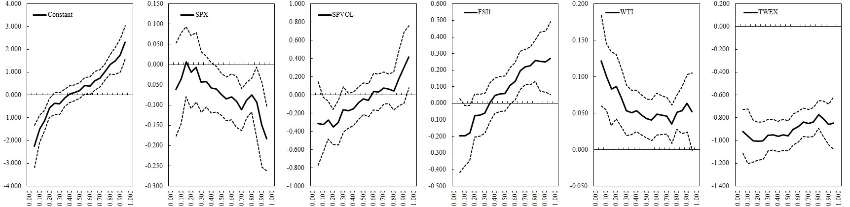
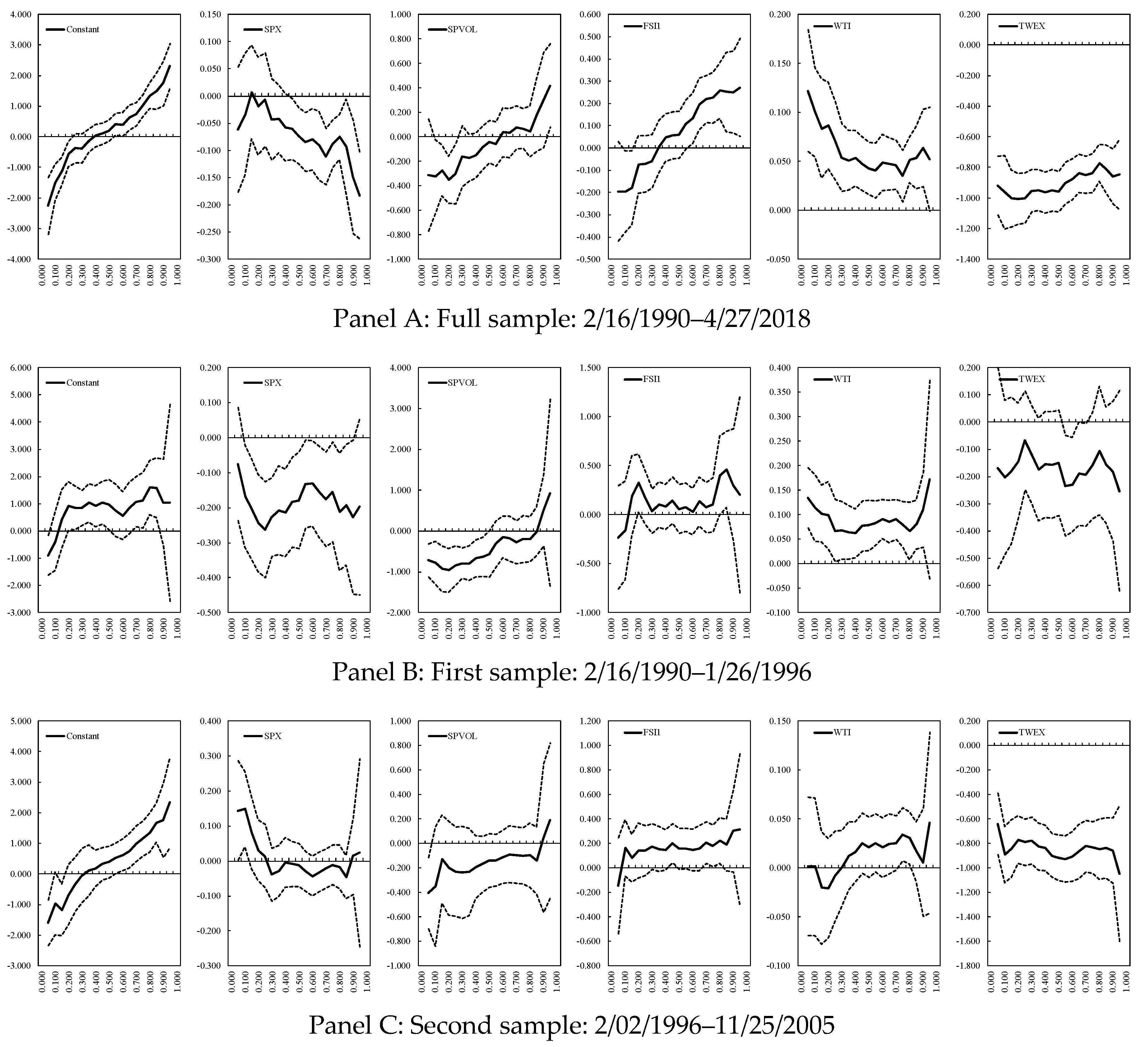
4.2. Quantile Regression Results

4.2.1. Full Sample Period

Our quantile regression model corresponding to Equation (5) is given by,

$$\begin{gathered} GOLD{\left(\tau \right)}_t={\beta }_0\left(\tau \right)+{\displaystyle \sum }_{i=1}^5{\beta }_i\left(\tau \right)GOL{D}_{t-i}+{\beta }_6\left(\tau \right)SP{X}_t+{\beta }_7\left(\tau \right)SPVO{L}_t+{\beta }_8\left(\tau \right)FSI{1}_t \\ +{\beta }_9\left(\tau \right)WT{I}_t+{\beta }_{10}\left(\tau \right)TWE{X}_t+e_t \end{gathered}$$

(6)

where $\tau$ indicates the quantile level. Each coefficient takes a different estimate according to the quantile level. By looking at each of the subsample periods, we can examine the change in the conditional joint distribution between gold return and each of financial indicators over time.

I present the estimation results for seven quantiles from 0.05 to 0.95 in

Table 6. Quantile process.

	Quantiles
	0.05	0.10	0.25	0.50	0.75	0.90	0.95
SPXfull	−0.062	−0.034	−0.007	−0.074 **	−0.088 **	−0.149 **	−0.183 **
	(0.059)	(0.057)	(0.044)	(0.026)	(0.022)	(0.053)	(0.040)
SPX1	−0.076	−0.166 *	−0.262 **	−0.179 *	−0.155 *	−0.227 *	−0.197
	(0.083)	(0.075)	(0.070)	(0.070)	(0.073)	(0.112)	(0.129)
SPX2	0.144 *	0.149 **	0.013	−0.012	−0.012	0.014	0.023
	(0.073)	(0.055)	(0.046)	(0.032)	(0.029)	(0.056)	(0.137)
SPX3	−0.061	−0.163	−0.082	−0.167	−0.337 **	−0.304 **	−0.222 **
	(0.087)	(0.108)	(0.068)	(0.089)	(0.085)	(0.065)	(0.072)
SPX4	−0.244	−0.267 **	−0.133	−0.087	0.034	−0.076	−0.060
	(0.174)	(0.102)	(0.116)	(0.075)	(0.097)	(0.101)	(0.081)
SPVOLfull	−0.313	−0.325 *	−0.302 *	−0.040	0.068	0.300	0.420 *
	(0.232)	(0.155)	(0.125)	(0.089)	(0.083)	(0.198)	(0.174)
SPVOL1	−0.716 **	−0.785 **	−0.845 **	−0.564	−0.202	0.508	0.924
	(0.207)	(0.267)	(0.246)	(0.290)	(0.293)	(0.446)	(1.179)
SPVOL2	−0.406 **	−0.352	−0.230	−0.139	−0.104	0.044	0.189
	(0.149)	(0.248)	(0.187)	(0.112)	(0.117)	(0.310)	(0.323)
SPVOL3	−0.549	−0.951 **	−0.378	0.116	0.382	0.593	0.341
	(0.343)	(0.238)	(0.195)	(0.370)	(0.269)	(0.306)	(0.375)
SPVOL4	0.060	0.162	0.248	0.045	0.089	0.135	−0.050
	(0.492)	(0.288)	(0.206)	(0.215)	(0.231)	(0.364)	(0.283)
FSI1full	−0.195	−0.196 *	−0.071	0.061	0.226 **	0.251 **	0.272 *
	(0.114)	(0.094)	(0.065)	(0.054)	(0.059)	(0.094)	(0.112)
FSI11	−0.232	−0.160	0.168	0.057	0.101	0.300	0.202
	(0.271)	(0.257)	(0.138)	(0.127)	(0.141)	(0.293)	(0.519)
FSI12	−0.144	0.164	0.142	0.156	0.180*	0.305	0.315
	(0.199)	(0.117)	(0.104)	(0.086)	(0.087)	(0.172)	(0.320)
FSI13	0.138	0.219	−0.026	−0.120	−0.068	−0.088	−0.034
	(0.325)	(0.159)	(0.107)	(0.124)	(0.127)	(0.168)	(0.250)
FSI14	−0.754	−0.620 *	−0.545 **	0.040	0.330	0.771 **	0.742 **
	(0.413)	(0.246)	(0.163)	(0.175)	(0.185)	(0.271)	(0.199)
WTIfull	0.122 **	0.100 **	0.071 **	0.043 **	0.035 **	0.064 **	0.052
	(0.032)	(0.023)	(0.020)	(0.014)	(0.013)	(0.020)	(0.027)
WTI1	0.134 **	0.114 **	0.067 *	0.078 **	0.080 **	0.110 **	0.171
	(0.032)	(0.035)	(0.033)	(0.026)	(0.024)	(0.039)	(0.104)
WTI2	0.001	0.001	−0.008	0.021	0.034 *	0.006	0.046
	(0.036)	(0.036)	(0.023)	(0.016)	(0.014)	(0.028)	(0.047)
WTI3	0.326 **	0.217 **	0.159 **	0.113	0.144 **	0.132 **	0.080
	(0.095)	(0.051)	(0.041)	(0.059)	(0.039)	(0.048)	(0.050)
WTI4	−0.010	−0.017	−0.059	−0.053	−0.058	−0.081	−0.149 **
	(0.080)	(0.049)	(0.040)	(0.034)	(0.051)	(0.107)	(0.055)
TWEXfull	−0.919 **	−0.961 **	−1.001 **	−0.958 **	−0.837 **	−0.858 **	−0.844 **
	(0.099)	(0.122)	(0.084)	(0.068)	(0.066)	(0.092)	(0.118)
TWEX1	−0.170	−0.204	−0.067	−0.150	−0.159	−0.180	−0.255
	(0.188)	(0.145)	(0.092)	(0.099)	(0.100)	(0.132)	(0.190)
TWEX2	−0.644 **	−0.891 **	−0.791 **	−0.917 **	−0.833 **	−0.858 **	−1.046 **
	(0.128)	(0.117)	(0.096)	(0.095)	(0.108)	(0.137)	(0.286)
TWEX3	−1.452 **	−1.591**	−1.551**	−1.661 **	−1.320 **	−1.103 **	−0.916 **
	(0.363)	(0.257)	(0.163)	(0.192)	(0.210)	(0.212)	(0.260)
TWEX4	−1.323 **	−1.445 **	−1.349 **	−1.167 **	−1.082 **	−0.773*	−0.637 **
	(0.237)	(0.245)	(0.156)	(0.160)	(0.164)	(0.317)	(0.211)
Constantfull	−2.254 **	−1.491 **	−0.371	0.204	1.021 **	1.750 **	2.320 **
	(0.470)	(0.304)	(0.242)	(0.176)	(0.182)	(0.372)	(0.374)
Constant1	−0.899 *	−0.390	0.851 *	0.966 *	1.125*	1.037	1.034
	(0.371)	(0.547)	(0.407)	(0.474)	(0.518)	(0.811)	(1.851)
Constant2	−1.592 **	−0.956	−0.330	0.393	1.162 **	1.757 **	2.348 **
	(0.385)	(0.524)	(0.453)	(0.265)	(0.293)	(0.622)	(0.755)
Constant3	−2.699 **	−0.589	−0.118	−0.045	1.157	1.943 **	3.243 **
	(0.776)	(0.462)	(0.370)	(0.702)	(0.595)	(0.623)	(0.832)
Constant4	−2.792 **	−2.255 **	−1.379 **	0.013	0.905 *	2.035 **	2.831 **
	(0.756)	(0.504)	(0.376)	(0.390)	(0.382)	(0.767)	(0.574)

Notes: The superscript letters “full,” ”1,” “2,” ”3,” and ”4” represent the periods for the full sample, first sample, second sample, third sample, and fourth sample, respectively. The numbers in parentheses below each coefficient estimate are the standard errors. * and ** denote statistical significance at the 5% and 1% levels, respectively.

. To compare the results visually, Figure 3 graphically illustrates all the quantile processes.

As shown in Panel A of Figure 3, Gold return is negatively correlated with the S&P 500 Index return and is significantly negative from the intermediate quantiles to the upper quantiles. The higher the quantile, the larger the coefficient increases in absolute value. The result means that gold return would rise largely when the stock return falls. However, the slope equality test at the lower and upper quantiles based on the Wald test cannot reject the null hypothesis of equality at 5% significance level, implying that dependence structures do not differ across quantile levels. Looking at the relationship with the stock return volatility, the estimated coefficient is negative for lower quantiles and positive for upper quantiles, implying that the gold return responds to the stock return volatility asymmetrically. The result that gold return rises as the stock market volatility increases is considered to reflect the investor behavior of divesting from stocks as a risky asset and demanding gold as a safety asset. Applying the Wald test, we can reject the slope equality hypothesis at 5% significance level, suggesting that dependence structures are different across quantile levels. Analogous to stock return volatility, for the financial market stress, the estimated coefficient is negative for the lower quantiles and positive for the upper quantiles, indicating asymmetric response of gold return to the degree of financial market stress. The Wald test clearly rejects the null hypothesis of equality at 1% significance level again. In other words, when the general financial market tightens, gold returns rise, and this result reflects the flight-to-quality behavior of investors.

Regarding the relationships with crude oil and the value of the US dollar, no noticeable difference is found from the results using OLS and robust regression. That is, the coefficient is significantly positive from lower to upper quantiles for crude oil, whereas it is significantly negative from lower to upper quantiles for the US dollar. The latter result is consistent with the findings of Miyazaki and Hamori (2016).

In summary, quantile regression allows us to clarify the responses of gold return on stock returns, stock market volatility, and financial market tightness in the tails of the distribution. Such relationships were not captured by OLS and robust regressions. In the following, we present detailed results for each subsample period.

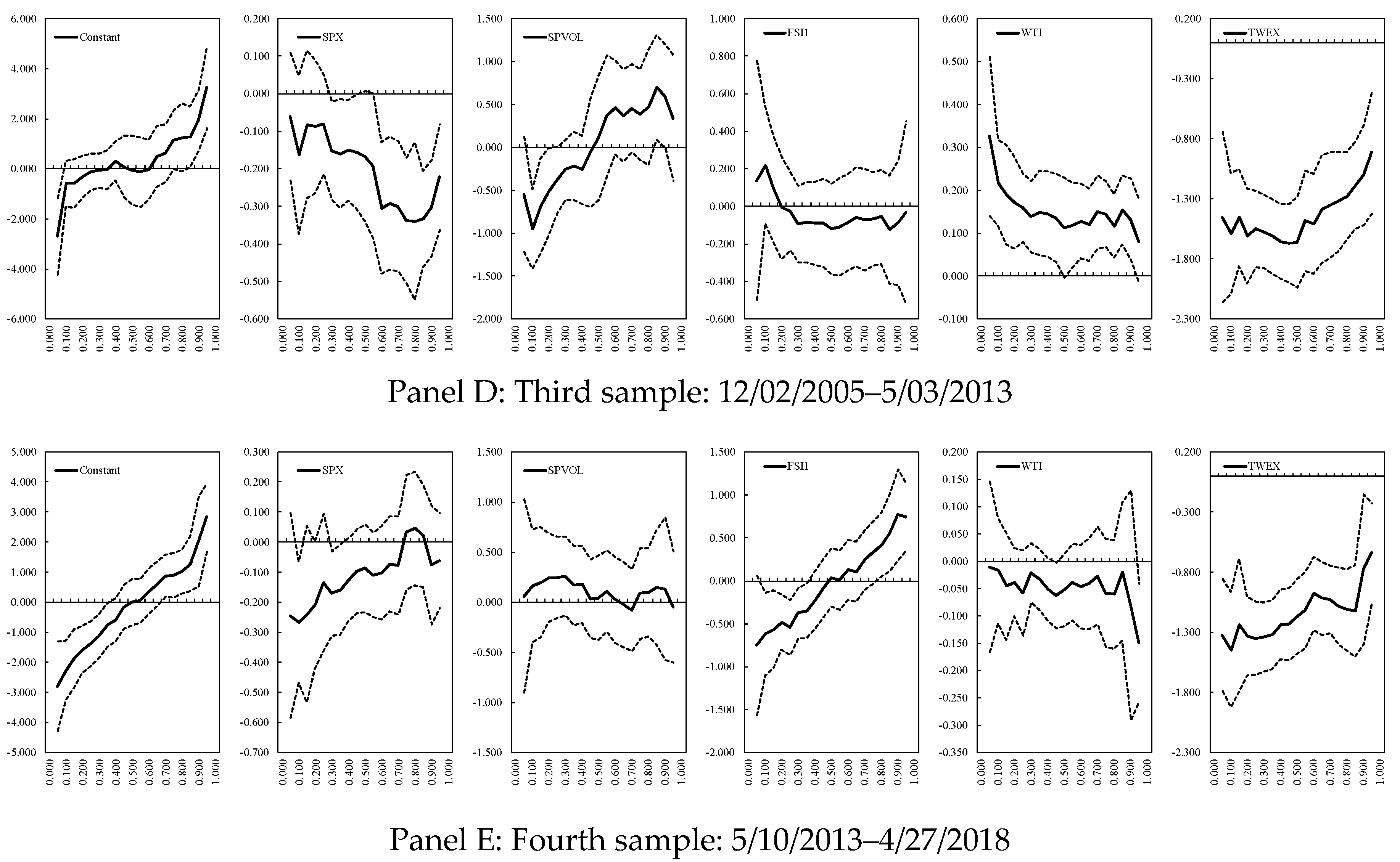
4.2.2. Subsample Periods

For every explanatory variable, the confidence intervals are widened at the upper quantiles. Gold return shows a constantly negative correlation with the S&P 500 Index return and with crude oil, regardless of quantile level. Gold return is negatively correlated with the stock return volatility at the lower quantiles. There is no remarkable relationship between gold return and financial market tightness and between gold return and the value of US dollar.

As in the first sample period, the confidence intervals are widened at the upper quantiles for every explanatory variable. We can observe a significant negative correlation between gold return and the value of the US dollar from the lower to the upper quantile, but no notable relationship is found for other explanatory variables.

Our third sample period covers the outbreak of the GFC. As seen in Figure 3, the results for this period are similar to those in the full sample period. The correlation between returns of gold and stock market is significantly negative from the intermediate quantiles to the upper quantiles. The negative coefficient tends to become larger as the quantile increases. Unlike the full sample period, however, the Wald test during this sample period rejects the null hypothesis of equality at the 5% significance level, indicating that dependence structures differ across quantile values. Likewise, for the relationship with the stock market volatility, we can observe a similar pattern to those in the whole sample. That is, the coefficient is negative in lower quantiles positive in the upper quantiles. However, the result of the Wald test shows that the null hypothesis of equality cannot be rejected marginally at the 5% significance level ($p\text{-value}=0.057$). Thus, we obtain partial evidence that flight to quality of investors from stock as a risky asset to gold as a safety asset had occurred.17 Similar arguments can be applied to crude oil and the value of US dollar. In other words, gold return is constantly and positively correlated with crude oil irrespective of quantile level and is negatively associated with the US dollar throughout the quantiles. Surprisingly, gold return does not respond significantly to the degree of general financial market stress throughout the quantiles.

Finally, we confirm the results in the sample period after the GFC. At the lower quantiles, gold return is negatively associated with the stock return. Meanwhile, we find no noticeable relation between gold return and stock return volatility and between gold return and crude oil. For the US dollar, similar to other subsample periods except the first one, there is a significant negative correlation from the lower quantiles to upper quantiles. A noteworthy feature in this sample period is that asymmetry is found in association with financial market risk; the coefficient is negative in the lower quantiles and positive in the upper quantiles. This result tells us that as the general financial market tightens, gold return rises. The Wald test also strongly reinforces this result. That is, the null hypothesis of equality is rejected at the 1% significance level. Thus, we can say that the flight to quality and the demand for gold as a safe haven by investors are phenomena that emerged recently. This finding is consistent with Baur (2011), but the findings of this study refer to a much later phenomenon.18

5. Conclusions

In this study, we investigate how gold returns respond to changes in financial variables such as stock returns and financial market conditions. In particular, in order to elaborate the behavior in the tails of the distribution, we use quantile regression to confirm that gold return exhibits an asymmetric response depending on the quantile level. Specifically, according to our empirical results, gold return rises when; (1) stock return falls, (2) stock market volatility increases, and (3) the general financial market tightens. Findings (1) and (2) are remarkable in the sample period covering the GFC and (3) is prominent in the sample after the GFC to the present. Furthermore, gold return shows almost constant positive correlation with crude oil, and negative correlation with the value of the US dollar. These results provide useful implications for portfolio selection of individual investors, risk management of financial institutions, and policymakers aiming for financial stability.

The analysis in this paper can be extended by explicitly incorporating the correlation with stock returns into the model, as in Connolly et al. (2005). They analyze the relationships between returns on stocks and bonds under a regime-switching framework. Furthermore, performing out-of-sample forecasting and evaluation of goodness of fit is also an important issue.19 Additionally, it is worth extending the model in this paper to predictive regression. Another way of extending of our analysis is to model the dependence structure by using copula or extreme value theory, which is now widely applied in the empirical finance literature. We leave these promising extensions for future research.

References

1. Agyei-Ampomah, Sam, Dimitrios Gounopoulos, and Khelifa Mazouz. 2014. Does gold offer a better protection against losses in sovereign debt bonds than other metals? Journal of Banking & Finance 40: 507–21. [Google Scholar]
2. Akram, Q. Farooq. 2009. Commodity prices, interest rates and the dollar. Energy Economics 31: 838–51. [Google Scholar] [CrossRef]
3. Alkhatib, Akram, and Murad Harasheh. 2018. Performance of Exchange Traded Funds during the Brexit referendum: An event study. International Journal of Financial Studies 6: 64. [Google Scholar] [CrossRef]
4. Alexander, Carol. 2008. Market Risk Analysis: Practical Financial Econometrics (Vol. II). Hoboken: Wiley. [Google Scholar]
5. Bai, Jushan, and Pierre Perron. 1998. Estimating and testing linear models with multiple structural changes. Econometrica 66: 47–78. [Google Scholar] [CrossRef]
6. Bai, Jushan, and Pierre Perron. 2003a. Computation and analysis of multiple structural change models. Journal of Applied Econometrics 18: 1–22. [Google Scholar] [CrossRef]
7. Bai, Jushan, and Pierre Perron. 2003b. Critical values for multiple structural change tests. The Econometrics Journal 6: 72–78. [Google Scholar] [CrossRef]
8. Balcilar, Mehmet, Zeynel Abidin Ozdemir, and Huseyin Ozdemir. 2018. Dynamic Return and Volatility Spillovers among S&P 500, Crude Oil and Gold. Discussion Paper 15–46. Famagusta: Eastern Mediterranean University, Department of Economics. [Google Scholar]
9. Basu, Parantap, and William T. Gavin. 2011. What explains the growth in commodity derivatives? Federal Bank of St. Louis Review 93: 37–48. [Google Scholar] [CrossRef]
10. Batten, Jonathan A., Cetin Ciner, and Brian M. Lucey. 2010. The macroeconomic determinants of volatility in precious metals markets. Resources Policy 35: 65–71. [Google Scholar] [CrossRef]
11. Batten, Jonathan A., Cetin Ciner, and Brian M. Lucey. 2014. Which precious metals spill over on which, when and why? Some evidence. Applied Economics Letters 22: 466–73. [Google Scholar] [CrossRef]
12. Baur, Dirk G. 2011. Explanatory mining for gold: Contrasting evidence from simple and multiple regressions. Resources Policy 36: 265–75. [Google Scholar] [CrossRef]
13. Baur, Dirk G. 2013. The structure and degree of dependence: A quantile regression approach. Journal of Banking & Finance 37: 786–98. [Google Scholar]
14. Baur, Dirk G., and Niels Schulze. 2005. Coexceedances in financial markets—A quantile regression analysis of contagion. Emerging Markets Review 6: 21–43. [Google Scholar] [CrossRef]
15. Baur, Dirk G., and Brian M. Lucey. 2010. Is gold a hedge or a safe haven? An analysis of stocks, bonds and gold. Financial Review 45: 217–29. [Google Scholar] [CrossRef]
16. Baur, Dirk G., and Thomas K. McDermott. 2010. Is gold a safe haven? International evidence. Journal of Banking & Finance 34: 1886–98. [Google Scholar]
17. Bhar, Ramaprasad, and Shawkat Hammoudeh. 2011. Commodities and financial variables: Analyzing relationships in a changing regime environment. International Review of Economics & Finance 20: 469–84. [Google Scholar]
18. Bouoiyour, Jamal, Refk Selmi, and Mark Wohar. 2018. Measuring the response of gold prices to uncertainty: An analysis beyond the mean. In Economic Modelling. Amsterdam: Elsevier, in press. [Google Scholar]
19. Chan, Kam Fong, Sirimon Treepongkaruna, Robert Brooks, and Stephen Gray. 2011. Asset market linkages: Evidence from financial, commodity and real estate assets. Journal of Banking & Finance 35: 1415–26. [Google Scholar]
20. Chao, Shih-Kang, Wolfgang K. Härdle, and Weining Wang. 2012. Quantile Regression in Risk Calibration. SFB 649 Discussion Paper 2012-006. Berlin: Humboldt-Universität. [Google Scholar]
21. Cheng, Ing-Haw, and Wei Xiong. 2014. Financialization of commodity markets. Annual Review of Financial Economics 6: 419–41. [Google Scholar] [CrossRef]
22. Chevallier, Julien, and Florian Ielpo. 2013. Volatility spillovers in commodity markets. Applied Economics Letters 20: 1211–27. [Google Scholar] [CrossRef]
23. Chudik, Alexander, and Marcel Fratzscher. 2011. Identifying the global transmission of the 2007–2009 financial crisis in a GVAR model. European Economic Review 55: 325–39. [Google Scholar] [CrossRef]
24. Ciner, Cetin, Constantin Gurdgiev, and Brian M. Lucey. 2013. Hedges and safe havens: An examination of stocks, bonds, gold, oil, and exchange rates. International Review of Financial Analysis 29: 202–11. [Google Scholar] [CrossRef]
25. Cohen, Gil, and Mahmod Qadan. 2010. Is gold still a shelter to fear? American Journal of Social and Management Sciences 1: 39–43. [Google Scholar] [CrossRef]
26. Connolly, Robert, Chris Stivers, and Licheng Sun. 2005. Stock market uncertainty and the stock-bond return relation. Journal of Financial and Quantitative Analysis 40: 161–94. [Google Scholar] [CrossRef]
27. Cont, Rama. 2001. Empirical properties of asset returns: Stylized facts and statistical issues. Quantitative Finance 1: 223–36. [Google Scholar] [CrossRef]
28. Diebold, Francis X., and Kamil Yilmaz. 2012. Better to give than to receive: Predictive directional measurement of volatility spillovers. International Journal of Forecasting 28: 57–66. [Google Scholar] [CrossRef] [Green Version]
29. Domanski, Dietrich, and Alexandra Heath. 2007. Financial investors and commodity markets. BIS Quarterly Review 3: 53–67. [Google Scholar]
30. Ehrmann, Michael, Marcel Fratzscher, and Roberto Rigobon. 2011. Stocks, bonds, money markets, and exchange rates: Measuring international financial transmission. Journal of Applied Econometrics 26: 948–74. [Google Scholar] [CrossRef]
31. Erb, Claude B., and Campbell R. Harvey. 2006. The strategic and tactical value of commodity futures. Financial Analysts Journal 62: 69–97. [Google Scholar] [CrossRef]
32. Fabozzi, Frank J., Sergio M. Focardi, Svetlozar T. Rachev, and Bala G. Arshanapalli. 2014. The Basics of Financial Econometrics: Tools, Concepts, and Asset Management Applications. Hoboken: John Wiley & Sons, Inc. [Google Scholar]
33. Franke, Jürgen, Peter Mwita, and Weining Wang. 2015. Nonparametric estimates for conditional quantiles of time series. AStA Advances in Statistical Analysis 99: 107–30. [Google Scholar] [CrossRef]
34. Gorton, Gary, and K. Geert Rouwenhorst. 2006. Facts and fantasies about commodity futures. Financial Analysts Journal 62: 47–68. [Google Scholar] [CrossRef]
35. Guo, Feng, Carl R. Chen, and Ying Sophie Huang. 2011. Markets contagion during financial crisis: A regime-switching approach. International Review of Economics & Finance 20: 95–109. [Google Scholar]
36. Hammoudeh, Shawkat, Ramazan Sari, and Bradley T. Ewing. 2009. Relationships among strategic commodities and with financial variables: A new look. Contemporary Economic Policy 27: 251–64. [Google Scholar] [CrossRef]
37. Hao, Lingxin, and Daniel Q. Naiman. 2007. Quantile Regression. Quantitative Applications in the Social Sciences, No. 149. Thousand Oaks: SAGE Publications, Inc. [Google Scholar]
38. Hartmann, Philipp, Stefan Straetmans, and C. G. de Vries. 2004. Asset market linkages in crisis periods. Review of Economics and Statistics 86: 313–26. [Google Scholar] [CrossRef]
39. Hillier, David, Paul Draper, and Robert Faff. 2006. Do precious metals shine? An investment perspective. Financial Analysts Journal 62: 98–106. [Google Scholar] [CrossRef]
40. Hood, Matthew, and Farooq Malik. 2013. Is gold the best hedge and a safe haven under changing stock market volatility? Review of Financial Economics 22: 47–52. [Google Scholar] [CrossRef]
41. IHS Global Inc. 2016. EViews 9 User’s Guide II. California: IHS Global Inc. [Google Scholar]
42. Koenker, Roger, and Gilbert Bassett Jr. 1978. Regression quantiles. Econometrica 46: 33–50. [Google Scholar] [CrossRef]
43. Koenker, Roger, and Kevin F. Hallock. 2001. Quantile regression. Journal of Economic Perspectives 15: 143–56. [Google Scholar] [CrossRef]
44. Longstaff, Francis A. 2010. The subprime credit crisis and contagion in financial markets. Journal of Financial Economics 97: 436–50. [Google Scholar] [CrossRef]
45. Mensi, Walid, Makram Beljid, Adel Boubaker, and Shunsuke Managi. 2013. Correlations and volatility spillovers across commodity and stock markets: Linking energies, food, and gold. Economic Modelling 32: 15–22. [Google Scholar] [CrossRef] [Green Version]
46. Mensi, Walid, Shawkat Hammoudeh, Juan C. Reboredo, and Duc K. Nguyen. 2014. Do global factors impact BRICS stock markets? A quantile regression approach. Emerging Markets Review 19: 1–17. [Google Scholar] [CrossRef]
47. Miyazaki, Takashi, and Shigeyuki Hamori. 2013. Testing for causality between the gold return and stock market performance: Evidence for “gold investment in case of emergency”. Applied Financial Economics 23: 27–40. [Google Scholar] [CrossRef]
48. Miyazaki, Takashi, and Shigeyuki Hamori. 2014. Cointegration with regime shift between gold and financial variables. International Journal of Financial Research 5: 90–97. [Google Scholar] [CrossRef]
49. Miyazaki, Takashi, and Shigeyuki Hamori. 2016. Asymmetric correlations in gold and other financial markets. Applied Economics 48: 4419–25. [Google Scholar] [CrossRef]
50. Miyazaki, Takashi, and Shigeyuki Hamori. 2018. The determinants of a simultaneous crash in gold and stock markets: An ordered logit approach. Annals of Financial Economics 13: 1850004. [Google Scholar] [CrossRef]
51. Miyazaki, Takashi, Yuki Toyoshima, and Shigeyuki Hamori. 2012. Exploring the dynamic interdependence between gold and other financial markets. Economics Bulletin 32: 37–50. [Google Scholar]
52. O’Connor, Fergal A., Brian M. Lucey, Jonathan A. Batten, and Dirk G. Baur. 2015. The financial economics of gold—A survey. International Review of Financial Analysis 41: 186–205. [Google Scholar] [CrossRef]
53. Piplack, Jan, and Stefan Straetmans. 2010. Comovements of different asset classes during market stress. Pacific Economic Review 15: 385–400. [Google Scholar] [CrossRef]
54. Qadan, Mahmod, and Joseph Yagil. 2012. Fear sentiments and gold price: Testing causality in-mean and in-variance. Applied Economics Letters 19: 363–66. [Google Scholar] [CrossRef]
55. Raza, Syed Ali, Nida Shah, and Muhammad Shahbaz. 2018. Does economic policy uncertainty influence gold prices? Evidence from a nonparametric causality-in-quantiles approach. Resources Policy 57: 61–68. [Google Scholar] [CrossRef]
56. Reboredo, Juan C., and Gazi Salah Uddin. 2016. Do financial stress and policy uncertainty have an impact on the energy and metals markets? A quantile regression approach. International Review of Economics & Finance 43: 284–98. [Google Scholar]
57. Renaud, Olivier, and Maria-Pia Victoria-Feser. 2010. A robust coefficient of determination for regression. Journal of Statistical Planning and Inference 140: 1852–62. [Google Scholar] [CrossRef]
58. Rodriguez, Robert N., and Yonggang Yao. 2017. Five Things You Should Know about Quantile Regression. Paper SAS525–2017. Cary: SAS Institute Inc. [Google Scholar]
59. Sari, Ramazan, Shawkat Hammoudeh, and Ugur Soytas. 2010. Dynamics of oil price, precious metal prices, and exchange rate. Energy Economics 32: 351–62. [Google Scholar] [CrossRef]
60. Silvennoinen, Annastiina, and Susan Thorp. 2013. Financialization, crisis, and commodity correlation dynamics. Journal of International Financial Markets, Institutions & Money 24: 42–65. [Google Scholar]
61. Straetmans, Stefan T. M., Willem F. C. Verschoor, and Christian C. P. Wolff. 2008. Extreme US stock market fluctuations in the wake of 9/11. Journal of Applied Econometrics 23: 17–42. [Google Scholar] [CrossRef] [Green Version]
62. Tang, Ke, and Wei Xiong. 2012. Index investment and the financialization of commodities. Financial Analysts Journal 68: 54–74. [Google Scholar] [CrossRef]
63. Wheelock, David C., and Mark E. Wohar. 2009. Can the term spread predict output growth and recessions? A survey of the literature. In Federal Reserve Bank of St. Louis Review 91. St. Louis: Federal Reserve Bank. [Google Scholar]
64. World Gold Council. 2010. Gold: Hedging against Tail Risk. London: World Gold Council. [Google Scholar]
1
Previous studies that analyze the financialization of commodities and its background include Basu and Gavin (2011); Cheng and Xiong (2014); Domanski and Heath (2007); Silvennoinen and Thorp (2013); Tang and Xiong (2012).
2
One of the other ways to disentangle the interdependence of data in the tails of the distribution is a method using extreme value theory. Related research includes Hartmann et al. (2004); Piplack and Straetmans (2010); Straetmans et al. (2008).
3
See Chapter 8 of Fabozzi et al. (2014).
4
EViews 9.5 is used for the robust regression in this study. For a more detailed technical description, refer to pp. 405-424 in IHS Global Inc. (2016).
5
For a succinct explanation of quantile regression, I recommend Koenker and Hallock (2001) and Rodriguez and Yao (2017). For more formal treatments, refer to textbooks such as Chapter II.7.2 of Alexander (2008), Chapter 7 of Fabozzi et al. (2014); Hao and Naiman (2007). For nonparametric approach of the quantile regression, see Chao et al. (2012); Franke et al. (2015).
6
We recognize its relevance, but exclude bond from our analysis since we consider that information in bond market is included, to some extent, in the financial market stress index constructed below. Existing studies explicitly demonstrating the connection of gold with bond include Agyei-Ampomah et al. (2014); Baur and Lucey (2010); Baur and McDermott (2010); Ciner et al. (2013); Miyazaki and Hamori (2016); Piplack and Straetmans (2010).
7
TED spread is calculated as the spread between the three-month London interbank offered rate based on US dollars and the three-month Treasury bill rate.
8
Credit spread is calculated as the yield spread between Baa- and Aaa-ranked corporate bonds.
9
Default spread is calculated as the yield spread between Aaa-ranked corporate bonds and Treasuries with 10-year constant maturities.
10
Term spread is calculated as the yield spread between Treasuries of 10-year and three-month constant maturities.
11
Before carrying out PCA, I standardized to control the variance of these variables. That is, these variables have zero mean and unit variance (standard deviation). Furthermore, according to the augmented Dickey–Fuller test, based on specification without a constant term, the null hypothesis of a unit root for these four variables is rejected at the 1% significance level or higher.
12
Several existing studies provide evidence that the term spread possesses significant predictive power as a leading indicator of recession. Wheelock and Wohar (2009) is a good survey in this area.
13
The lag order for both the ARCH and GARCH terms in the EGARCH model is 1, namely, EGARCH (1,1).
14
Taking into account the autocorrelation of the residuals, we include the autoregressive term up to five lags. For the sake of brevity, we do not explicitly mention the autoregressive term in the empirical analysis below.
15
The null hypothesis of “no structural break” is also rejected in the Chow test which designated jointly and beforehand three structural breakpoints identified by Bai and Perron’s (1998, 2003a, 2003b) test as a candidate of structural breakpoints. Therefore, these structural breakpoints identified above have robustness.
16
Miyazaki and Hamori (2014) demonstrate that there is a cointegrating relation with regime shift between gold and the three financial variables, namely US short-term interest rates, US dollar, and S&P 500 Index based on daily data. They identify a structural break date on 13 December 2005.
17
See also Miyazaki and Hamori (2013). They show that there exists a unilateral causality in not only the mean but the variance from stock return to gold return in the sample period post subprime crisis.
18
Although we do not dwell in the main text on the details of the results using FSI2, FSI3, and FSI4 as a financial stress index, all results are available from the author upon request.
19
I would like to thank an anonymous referee for raising this point.
Figure 1. FSI1 to FSI4 are the first to fourth principal components obtained by applying principal component analysis to the set of financial risk indicators; TED, Aaa-10Y, Baa-Aaa, and TERM. Here, TED is Ted spread, Aaa-10Y is the yield spread between Aaa-ranked corporate bonds and Treasuries with 10-year constant maturities (default spread), Baa-Aaa is the yield spread between Baa-ranked and Aaa-ranked corporate bonds (credit spread), and TERM is the yield spread between Treasuries of 10-year and three-month constant maturities. We interpret these four principal components as follows. FSI1: Degree of stress in general financial markets. FSI2: Financial tightening in the banking sector or a surge in liquidity risk. FSI3: Monetary policy stance or recession risk. FSI4: Risk premium on corporate bond with a relatively high credit.
Jrfm 12 00033 g001aJrfm 12 00033 g001b
Figure 2. The solid vertical lines in the figure represent the break dates specified by applying Bai and Perron’s (1998, 2003a, 2003b) method.
Jrfm 12 00033 g002
Figure 3. This graph illustrates the quantile process of gold return. For each panel, from left to right, we show the evolutions of coefficient on constant term, S&P 500 index return, S&P 500 Index return volatility, financial market stress, crude oil return, and the appreciation/depreciation rate of the trade-weighted US dollar. The dotted lines in the figure represent the 95% confidence intervals.
Jrfm 12 00033 g003aJrfm 12 00033 g003b