Threshold Stochastic Conditional Duration Model for Financial Transaction Data

Abstract

This paper proposes a variant of a threshold stochastic conditional duration (TSCD) model for financial data at the transaction level. It assumes that the innovations of the duration process follow a threshold distribution with a positive support. In addition, it also assumes that the latent first-order autoregressive process of the log conditional durations switches between two regimes. The regimes are determined by the levels of the observed durations and the TSCD model is specified to be self-excited. A novel Markov-Chain Monte Carlo method (MCMC) is developed for parameter estimation of the model. For model discrimination, we employ deviance information criteria, which does not depend on the number of model parameters directly. Duration forecasting is constructed by using an auxiliary particle filter based on the fitted models. Simulation studies demonstrate that the proposed TSCD model and MCMC method work well in terms of parameter estimation and duration forecasting. Lastly, the proposed model and method are applied to two classic data sets that have been studied in the literature, namely IBM and Boeing transaction data.

1. Introduction

In this paper,1 we propose a threshold Stochastic Conditional Duration (TSCD) model, in which the innovation of a financial duration process is assumed to follow a threshold distribution, where the two component distributions have positive supports, while the log duration process is kept to be the same as that in the classic Stochastic Conditional Duration (SCD) models introduced by Bauwens and Veredas (2004). In addition, we also assume that the state (i.e., the logarithm of the conditional durations) follows a threshold AR(1) process with the threshold level being driven by observed duration processes. The regimes are determined by a threshold parameter, which is estimated from the data. Suitable Markov-Chain Monte Carlo (MCMC) methods are developed within a Bayesian framework in which the parameters of the model and the augmented parameters, being the latent states, are estimated simultaneously by the estimation process. For the in-sample and out-of-sample duration forecasting, we use an auxiliary particle filter (APF) proposed in Pitt and Shephard (1999), from which the filter and predictive distributions of the latent states are approximated by samples of particles from the corresponding distributions. The APF is an efficient method for calculating the marginal likelihood of observed data. For model selection and comparison, we employ a deviance information criterion (DIC) proposed by Spiegelhalter et al. (2002).

The remaining parts of this paper are organized as follows. Section 2 introduces the TSCD model. In Section 3, we propose a suitable MCMC method for parameter estimation of the models with a Gamma distribution or a Weibull distribution serving as the component distributions in the model. The latent states are augmented as parameters and estimated as a by-product of the MCMC estimation processes. We simulate the state variables by using a single-move Metropolis-Hastings (MH) algorithm with a univariate normal distribution as the proposal. In Section 4, model diagnostics, model selection, and duration forecasting are presented and discussed. In particular, model assessment is performed by calculating probability integral transforms (PITs) produced from the fitted TSCD models. In Section 5, we conduct simulation studies to assess the performance of the proposed TSCD models and developed estimation methods, while in Section 6 we present empirical results from applications of the proposed TSCD models to two classic/benchmark data sets of IBM and Boeing transactions. In this section, restricted versions of the TSCD models are also estimated and analyzed. Concluding remarks are made in Section 7.

2. Threshold Stochastic Conditional Duration Model

Let $y_t$ denote the observed duration at time t, $t\le T$, where T is a positive integer representing the sample size. The duration process of $y_t$ is characterized by a product of two independent random variables: a lognormal random variable $H_t$ and a positive random variable ${ϵ}_t$. Then, following Bauwens and Veredas (2004), we specify the following set of equations:

$$\begin{array}{ccc}\hfill y_t& =H_t{ϵ}_t,H_t=exp\left(h_t\right),\hfill & \hfill t=1,\dots ,T,\end{array}$$

(1)

$$\begin{array}{ccc}\hfill h_{t+1}& =\mu +\varphi (h_t-\mu )+\sigma u_{t+1},\hfill & \hfill t=1,\dots ,T-1,\end{array}$$

(2)

$$\begin{array}{cc}\hfill h_1& \sim \mathcal{N}(\mu ,{\sigma }^2/(1-{\varphi }^2)),\hfill \end{array}$$

(3)

where ${ϵ}_t$ and $u_t$ are assumed to be mutually independent shocks with $u_t\sim \mathcal{N}(0,1)$. For the latent AR(1) process in (2) to be weakly stationary, it is assumed that $\left|\varphi \right|<1$. Bauwens and Veredas (2004) assume that ${ϵ}_t$ follows either a Gamma distribution or a Weibull distribution with scale parameters equal to 1.

In our proposed model, we allow not only the innovation of the duration process to follow a threshold distribution with two component distributions with positive supports, but also the latent states to follow a threshold AR(1) process which switches between two regimes. These two regimes are determined by the previously observed durations according to a threshold level. In particular, the threshold distribution for the innovations of the measurement equation is given by

$$\begin{array}{cc}\hfill & \left\{\begin{array}{cc}{ϵ}_t\sim {\mathcal{D}}_1\left({\delta }_1\right),\hfill & \mathrm{if}{y}_{t-1}\le r,\hfill \\ {ϵ}_t\sim {\mathcal{D}}_2\left({\delta }_2\right),\hfill & \mathrm{if}{y}_{t-1}>r,\hfill \end{array}\right.\hfill \end{array}$$

(4)

where ${\mathcal{D}}_1\left({\delta }_1\right)$ and ${\mathcal{D}}_2\left({\delta }_2\right)$ are two generic distributions with positive supports, and ${\delta }_1$ and ${\delta }_2$ are the corresponding parameter vectors.

For the log conditional durations, $h_t$, a threshold AR(1) process is defined as:

$$\begin{array}{cc}\hfill & \left\{\begin{array}{cc}{h}_{t+1}-{\mu }_1={\varphi }_1(h_t-{\mu }_1)+{\sigma }_1{u}_{1,t+1},\hfill & \mathrm{if}{y}_t\le r,\hfill \\ h_{t+1}-{\mu }_2={\varphi }_2(h_t-{\mu }_2)+{\sigma }_2{u}_{2,t+1},\hfill & \mathrm{if}{y}_t>r,\hfill \end{array}\right.\hfill \end{array}$$

(5)

where $u_{1,t+1}$ and $u_{2,t+1}$ are two independent processes with a standard normal distribution. In the threshold specification in (5), the latent states, $h_t$, follow separate AR(1) processes in the two different regimes determined by the previously observed duration $y_t$ and the threshold level r. The threshold level r is treated as a free parameter to be estimated by our proposed MCMC method.

For the components of the threshold distribution of ${ϵ}_t$, following Bauwens and Veredas (2004), we use either a Gamma distribution or a Weibull distribution. With this assumption, the probability density functions (pdfs) of ${ϵ}_t$ are given respectively by

$$\begin{array}{cc}\hfill & \left\{\begin{array}{cc}{f}_1\left({ϵ}_t\right)=\frac{1}{\Gamma \left({\gamma }_1\right)}{ϵ}_t^{{\gamma }_1-1}exp\{-{ϵ}_t\},\hfill & \mathrm{if}{y}_{t-1}\le r,\hfill \\ f_2\left({ϵ}_t\right)=\frac{1}{\Gamma \left({\gamma }_2\right)}{ϵ}_t^{{\gamma }_2-1}exp\{-{ϵ}_t\},\hfill & \mathrm{if}{y}_{t-1}>r,\hfill \end{array}\right.\hfill \end{array}$$

(6)

with the shape parameters ${\gamma }_1>0$ and ${\gamma }_2>0$, and the scale parameters are all set to 1, and

$$\begin{array}{cc}\hfill & \left\{\begin{array}{cc}{f}_1\left({ϵ}_t\right)=v_1{ϵ}_t^{v_1-1}exp\{-{ϵ}_t^{v_1}\},\hfill & \mathrm{if}{y}_{t-1},\le r,\hfill \\ f_2\left({ϵ}_t\right)=v_2{ϵ}_t^{v_2-1}exp\{-{ϵ}_t^{v_2}\},\hfill & \mathrm{if}{y}_{t-1},>r,\hfill \end{array}\right.\hfill \end{array}$$

(7)

with the shape parameters $v_1>0$ and $v_2>0$ and unit scale parameters. Under these assumptions, the distribution of ${ϵ}_t$ depends on the shape parameters. At time t, the observation $y_t$ affects not only the distribution of ${ϵ}_{t+1}$, but also the distribution of $h_{t+1}$. In other words, the observation, $y_t$, contributes to future durations through ${ϵ}_{t+1}$ and $h_{t+1}$. The asymmetric property of the marginal distribution of $y_{t+1}$ is influenced by the previously observed duration according to the threshold level r. Importantly, under the threshold distributional assumption, we no longer need to explicitly specify a correlation structure between the observation and the latent process. In addition, as the variance of ${ϵ}_t$ is not equal to 1, the location parameters in the threshold AR(1) processes are no longer required as well.

Under the TSCD model setup, at each time t, the conditional distribution of $y_t$ is assumed to depend on the previous observation $y_{t-1}$ and the threshold parameter r, i.e., the distributions of the observations will switch between the two regimes with the arrivals of the previously observed durations. Similar to the arguments in De Luca and Gallo (2004, 2009), who work with Autoregressive Conditional Duration (ACD) models, the two regimes can be interpreted as representing two types of behavior of traders in the market, who are respectively informed and uninformed traders. The informed and uninformed traders are assumed to respond differentially to bad news and good news in the market over the sample period. The proposed TSCD models with two regimes are constructed specifically to characterize these time dependent responses, giving rise to a desirably asymmetric pattern in the marginal distributions of the model.

3. Bayesian Inference

In this section, we develop a suitable MCMC method for parameter estimation of the proposed model. Following the literature, all the latent states, $h_t$, are augmented as parameters and simulated or estimated as a by-product of the derived estimators. For each specified TSCD model, the latent states are simulated one at a time by the slice sampler introduced by Neal (2003).

In the following MCMC algorithm, we assume that the innovation of the mean equation follows a threshold distribution with two, say Gamma, component distributions with $\theta =({\varphi }_1,{\sigma }_1,{\varphi }_2,{\sigma }_2,{\gamma }_1,{\gamma }_2,r)$ serving as the parameter vector. Given an observed duration time series of $\mathbf{y}=(y_1,\dots ,y_T)$, the conditional densities of $y_t$ are given by

$$\begin{array}{c}\hfill \left\{\begin{array}{cc}f\left(y_t\right|y_{t-1},h_t,r)=\frac{1}{\Gamma \left({\gamma }_1\right)}exp(-{\gamma }_1{h}_t)y_t^{{\gamma }_1-1}exp\left\{-y_{t}exp(-h_t)\right\},\hfill & \mathrm{if}{y}_{t-1}\le r,\hfill \\ f\left(y_t\right|y_{t-1},h_t,r)=\frac{1}{\Gamma \left({\gamma }_2\right)}exp(-{\gamma }_2{h}_t)y_t^{{\gamma }_2-1}exp\left\{-y_{t}exp(-h_t)\right\},\hfill & \mathrm{if}{y}_{t-1}>r.\hfill \end{array}\right.\end{array}$$

(8)

Therefore, the posterior density of $(\theta ,\mathbf{h})$ can be conveniently split into two parts according to the threshold parameter r,

$$\begin{array}{cc}\hfill f(\theta ,\mathbf{h}|\mathbf{y})& \propto \prod _{t=2,y_{t-1}\le r}^T\left[\frac{1}{\Gamma \left({\gamma }_1\right)}exp(-{\gamma }_1{h}_t)y_t^{{\gamma }_1-1}exp\left\{-y_{t}exp(-h_t)\right\}\right]\hfill \\ & \times \prod _{t=2,y_{t-1}>r}^T\left[\frac{1}{\Gamma \left({\gamma }_2\right)}exp(-{\gamma }_2{h}_t)y_t^{{\gamma }_2-1}exp\left\{-y_{t}exp(-h_t)\right\}\right],\hfill \end{array}$$

(9)

where $\mathbf{h}=(h_1,\dots ,h_T)$. Within the Bayesian inference, the posterior distributions of the parameters in $\theta$, and the latent states, $\mathbf{h}$, can be readily derived from (9).

The TSCD model is completed by specifying prior distributions for all the parameters in $\theta$. For tractability, we assume that the prior distributions of the parameters in $\theta$ are mutually independent. The persistence parameters ${\varphi }_1$ and ${\varphi }_2$ are assumed to have a univariate normal distribution ${\varphi }_i\sim N(0,5),i=1,2$, truncated in the interval $(-1,1)$. Instead of sampling ${\sigma }_1$ and ${\sigma }_2$, we sample ${\sigma }_1^2$ and ${\sigma }_2^2$. The prior distributions of ${\sigma }_1^2$ and ${\sigma }_2^2$ are ${\sigma }_i^2\sim IG(0.25,5),i=1,2$, which are inverse Gamma distributions. For the shape parameters ${\gamma }_1$ and ${\gamma }_2$ we use the half-Cauchy distributions as their prior distributions

$$\begin{array}{c}\hfill f\left({\gamma }_i\right)\propto \frac{1}{1+{\gamma }_i^2},{\gamma }_i>0,i=1,2.\end{array}$$

(10)

The half-Cauchy distribution is also used as the prior distribution for the shape parameters of the Weibull components. For the threshold parameter r, we use a uniform distribution between the first and third quartiles of the observations in $\mathbf{y}$. The two quartiles are intended to ensure that there are enough observations in each of the two regimes.

The algorithm of the MCMC estimation procedure for the TSCD model with a threshold Gamma distribution, called TSCD-G model hereafter, is listed in Algorithm 1. The derivation of the full conditionals for the parameters and individual latent state are given explicitly in Step 1 below, where the full conditional of each parameter is defined as the conditional distribution given that other parameters in the model have been sampled.

Algorithm 1: MCMC algorithm for the TSCD-G model.

Step 0. Initialize $\mathbf{h}$, ${\varphi }_i$, ${\sigma }_i$, ${\gamma }_i$, i=1, 2, and r  Step 1. Sample $h_t,t=2,\dots ,T$  Step 2. Sample ${\gamma }_1$ and ${\gamma }_2$  Step 3. Sample r  Step 4. Sample ${\varphi }_i$ and ${\sigma }_i^2,i=1,2$  Step 5. Go to Step 1.

Step 0. Initialize $\mathbf{h}$, ${\varphi }_i$, ${\sigma }_i$, ${\gamma }_i$ and r. To start the MCMC algorithm, the initial values of the parameters of the model are set as ${\varphi }_1=0.5$, ${\varphi }_2=0.5$, ${\sigma }_1=0.12$, ${\sigma }_2=0.12$, ${\gamma }_1=0.5$, ${\gamma }_2=1.5$, $v_1=0.5$ and $v_2=1.5$. The initial value of r is set as the mean of the observations, which falls into the interval of the first and third quartiles of the observations. The initial values of $\mathbf{h}$ are generated from the latent AR(1) process with the above initial parameters.

Step 1. Sample $\mathbf{h}$. Here, we only give the full conditionals of $h_t$, $t=3,\dots T-1$. The full conditionals of $h_2$ and $h_T$ are easy to derive and, thus, omitted from this paper. The full conditional of $h_t$ depends on $y_{t+1},y_t,y_{t-1},h_{t+1},h_{t-1}$ and r. Given that r has been sampled previously, the full conditional of $h_t$ can be calculated based on four cases: (i) If $y_t\le r$ and $y_{t-1}\le r$, the full conditional of $h_t$ is given by

$$\begin{array}{c}f\left(h_t\right|h_{t-1},h_{t+1},y_t,{\theta }_{-r},y_t\le r,y_{t-1}\le r)\hfill \\ \propto f\left(y_t\right|h_t,{\theta }_{-r},y_{t-1}\le r)f\left(h_t\right|h_{t-1},y_{t-1}\le r,{\theta }_{-r})f\left(h_t\right|y_t\le r,h_{t+1},{\theta }_{-r})\hfill \\ \propto exp(-{\gamma }_1{h}_t)exp\left\{-y_{t}exp(-h_t)\right\}\hfill \\ \times exp\left\{-\frac{{\left(h_t-{\varphi }_1{h}_{t-1}\right)}^2}{2{\sigma }_1^2}\right\}\times exp\left\{-\frac{{\left(h_{t+1}-{\varphi }_1{h}_t\right)}^2}{2{\sigma }_1^2}\right\}\hfill \\ \propto exp\left\{-y_{t}exp(-h_t)\right\}\times exp\left\{-\frac{{\left(h_t-{\mu }_t\right)}^2}{2{\sigma }_t^2}\right\},\hfill \end{array}$$

(11)

where

$$\begin{array}{ccc}\hfill {\mu }_t& =-{\sigma }_t^2{\gamma }_1+\frac{{\varphi }_1(h_{t+1}+h_{t-1})}{1+{\varphi }_1^2},\hfill & \hfill {\sigma }_t^2=\frac{{\sigma }_1^2}{1+{\varphi }_1^2}.\end{array}$$

Here ${\theta }_{-r}$ defines as a collection of model parameters except for r. Thus, the full conditional of $h_t$ can be sampled by the slice sampler.

Algorithm of the slice sampler for ${\mathbf{h}}_{\mathit{t}}$

SS1. 

Draw $u_1$ uniformly from the interval $(0,1)$ and set $u_2=u_{1}exp\left\{-\frac{{\left(h_t-{\mu }_t\right)}^2}{2{\sigma }_t^2}\right\}$. Let $u_2<exp\{-\frac{{\left(h_t-{\mu }_t\right)}^2}{2{\sigma }_t^2}\}$, then we have

$$\begin{array}{c}\hfill {\mu }_t-\sqrt{-2{\sigma }_t^{2}log\left(u_2\right)}<h_t<{\mu }_t+\sqrt{-2{\sigma }_t^{2}log\left(u_2\right)}.\end{array}$$

(12)

SS2. 

Draw $u_3$ uniformly from the interval $(0,1)$ and set $u_4=u_{3}exp\left\{-y_{t}exp(-h_t)\right\}$. Let $u_4<exp\left\{-y_{t}exp(-h_t)\right\}$ then we have

$$\begin{array}{cc}\hfill h_t& >-log(-log\left(u_4\right)/y_t)\hfill \end{array}$$

SS3. 

Draw $h_t$ uniformly from the interval determined by the inequalities in (11) and (12) such as

$$\begin{array}{c}\hfill h_t\sim U\left(max\left\{-log(-log\left(u_4\right)/y_t),{\mu }_t-\sqrt{-2{\sigma }_t^{2}log\left(u_2\right)}\right\},{\mu }_t+\sqrt{-2{\sigma }_t^{2}log\left(u_2\right)}\right).\end{array}$$

As a brief remark to the above algorithm, we note that in our approach, each $h_t$ is simulated based on its conditional distribution. So conditionally ${\mu }_t$ is known in our situation. Also note that $y_{t+1}$’s are the only observations available to our model. As we subsequently perform a one-step-ahead prediction for the fitted model, we only need to sample $h_{t+1}$, and do not need to sample $y_{t+1}$.

In each MCMC iteration, when we simulate $h_t$, the sampled value of $h_t$ from the previous MCMC step is set at the initial value. As the full conditionals of $h_t$ in each MCMC step are similar, this initial value should provide a good starting point. As the slice sampler adapts to the form of the density function of the underlying variable, it is more efficient than many other existing samplers. In addition, under certain conditions, Roberts and Rosenthal (1999) also show that the slice algorithm is robust and has geometric periodicity properties. Moreover, Mira and Tierney (2002) prove that the slice sampler has a smaller second-largest eigenvalue, which ensures faster convergence to the underlying distribution. Indeed, in our study, we find that even with only five iterations of our slice algorithm, we can feasibly and efficiently estimate the TSCD models by the MCMC.2

The single-move simulation method is popular in the literature and used in Jacquier et al. (2004); Yu et al. (2006); Zhang and King (2008), Men et al. (2015, 2016a, 2016b) among others. The advantage of the slice sampler is that five iterations can give us a point from the underlying distribution unlike the MH algorithm where many generated points must be discarded.

The full conditional of $h_t$, given (ii) $y_t>r$ and $y_{t-1}\le r$, is

$$\begin{array}{c}f\left(h_t\right|h_{t-1},h_{t+1},y_t,{\theta }_{-r},y_t>r,y_{t-1}\le r)\hfill \\ \propto f\left(y_t\right|h_t,{\theta }_{-r},y_{t-1}\le r)f\left(h_t\right|h_{t-1},y_{t-1}\le r,{\theta }_{-r})f\left(h_t\right|y_t>r,h_{t+1},{\theta }_{-r})\hfill \\ \propto exp(-{\gamma }_1{h}_t)exp\left\{-y_{t}exp(-h_t)\right\}\hfill \\ \times exp\left\{-\frac{{\left(h_t-{\varphi }_1{h}_{t-1}\right)}^2}{2{\sigma }_1^2}\right\}exp\left\{-\frac{{\left(h_{t+1}-{\varphi }_2{h}_t\right)}^2}{2{\sigma }_2^2}\right\}\hfill \\ \propto exp\left\{-y_{t}exp(-h_t)\right\}\times exp\left\{-\frac{{\left(h_t-{\mu }_t\right)}^2}{2{\sigma }_t^2}\right\},\hfill \end{array}$$

(13)

where

$$\begin{array}{ccc}\hfill {\mu }_t& =-{\gamma }_1{\sigma }_t^2+\frac{a}{b},\hfill & \hfill {\sigma }_t^2=\frac{1}{b}\\ \hfill \mathrm{with}a& =\frac{{\varphi }_{1}h{}_{t-1}}{{\sigma }_1^2}+\frac{{\varphi }_{2}h{}_{t+1}}{{\sigma }_2^2},\hfill & \hfill b=\frac{1}{{\sigma }_1^2}+\frac{{\varphi }_2^2}{{\sigma }_2^2}.\end{array}$$

The full conditional of $h_t$ is also sampled through the slice sampler. Under the other conditions (iii) $y_t>r$ and $y_{t-1}>r$, and (iv) $y_t\le r$ and $y_{t-1}>r$, the full condition of $h_t$ can be calculated in the same fashion, and the realized full conditionals of $h_t$ can be sampled through the slice sampler.

Step 2. Sample ${\gamma }_1$ and ${\gamma }_2$. Given that other parameters and the latent states have been sampled from the previous iteration of the MCMC algorithm, the full conditionals of ${\gamma }_i$, $i=1,2$, are given respectively by

$$\begin{array}{cc}\hfill f\left({\gamma }_1\right|\mathbf{y},\mathbf{h},{\theta }_{-{\gamma }_1})& \propto \prod _{t=2,y_{t-1}\le r}^T\left(\frac{exp(-{\gamma }_1{h}_t)}{\Gamma \left({\gamma }_1\right)}{y}_t^{{\gamma }_1-1}\right)\frac{1}{1+{\gamma }_1^2},\hfill \end{array}$$

(14)

$$\begin{array}{cc}\hfill f\left({\gamma }_2\right|\mathbf{y},\mathbf{h},{\theta }_{-{\gamma }_2})& \propto \prod _{t=2,y_{t-1}>r}^T\left(\frac{exp(-{\gamma }_2{h}_t)}{\Gamma \left({\gamma }_2\right)}{y}_t^{{\gamma }_2-1}\right)\frac{1}{1+{\gamma }_2^2}.\hfill \end{array}$$

(15)

These distributions are not simple distributions that can be simulated directly. Our simple solution to this is to use a random-walk MH method with a univariate normal distribution with mean zero and non-unit variance. The variance can be fined tuned to obtain a reasonable acceptance rate for the MH algorithm. Experience from our study suggests that an acceptance rate between 25% and $55\%$ gives us a more accurate estimate of r in the simulation studies.

Step 3. Sample r. The full conditional of r is

$$\begin{array}{c}f\left(r\right|\mathbf{y},\mathbf{h},{\theta }_{-r})\hfill \\ \propto \prod _{t=2,y_{t-1}\le r}^T\left(\frac{exp(-{\gamma }_1{h}_t)y_t^{{\gamma }_1-1}}{\Gamma \left({\gamma }_1\right)}\right)\prod _{t=2,y_{t-1}>r}^T\left(\frac{exp(-{\gamma }_2{h}_t)y_t^{{\gamma }_2-1}}{\Gamma \left({\gamma }_2\right)}\right).\hfill \end{array}$$

(16)

The full conditional of r is not a simple distribution either. Therefore, again, we use a random-walk MH method to simulate this posterior distribution with a univariate normal distribution $N(0,{\sigma }_0^2)$, where ${\sigma }_0$ is fined tuned for the random-walk MH method to have a reasonable acceptance rate.

Step 4. Sample ${\varphi }_1$, ${\varphi }_2$, ${\sigma }_1^2$ and ${\sigma }^2$. The full conditionals of ${\varphi }_i$ are univariate normal distributions truncated in the interval (−1,1), which can be simulated by a slice sampler. The full conditionals of ${\sigma }_i^2$ are inverse Gamma distributions from which the sampling is relatively easy to carry out. The derivation of these full conditionals are not given in this paper, but they can be found for instance in Men et al. (2016a) or any in prior studies on SV models such as Men et al. (2016b), where MCMC algorithms are used.

To conduct a Bayesian inference in the TSCD model with threshold Weibull component distributions, the estimation algorithm can be derived similarly. As a result, details of these derivations are omitted from the paper.

4. Model Selection, Assessment and Duration Forecasting

4.1. Model Selection

Information criteria such as AIC due to Akaike (1987) and BIC due to Schwarz (1978) are often used for model comparison. For instance, in the study of SV models, Lopes and West (2004) and Zhang and King (2008) use the AIC and the BIC for model selection. It is well-known that the AIC tends to choose a model with a larger number of parameters, while the BIC tends to prefer a model with a smaller number of parameters. It is important to note that in the calculation of the AIC and the BIC, we need to know the exact number of parameters of the model. For hidden Markov models such as the TSCD models proposed in this paper, the number of parameters is difficult to determine since all the latent states are augmented as parameters and highly correlated. For instance, when a TSCD-G model is fitted to a data set with T observations, the number of parameters in the fitted model could be (T + 7) or less. However, it is worth reiterating that the AIC and the BIC are functions of both the number of parameters and the sample size. This indicates that the AIC and the BIC are not suitable for discriminating hidden Markov models, including the TSCD models. A new criterion, called the DIC proposed by Spiegelhalter et al. (2002) is used in this paper to discriminate between these models since it does not depend on the number of parameters directly. The DIC is defined as follows:

$$\begin{array}{cc}\hfill \mathrm{DIC}& =\overline{D}+P_D.\hfill \end{array}$$

The first term

$$\begin{array}{c}\overline{D}(\theta ,\mathbf{h})=E_{\theta ,\mathbf{h}|\mathbf{y}}\left[D(\theta ,\mathbf{h})\right],\mathrm{where}D(\theta ,\mathbf{h})=-2logf\left(\mathbf{y}\right|\theta ,\mathbf{h}),\hfill \end{array}$$

represents a Bayesian measure of a model fit. It is called the posterior mean of the deviance. The second term is

$$\begin{array}{cc}\hfill P_D& =\overline{D}-D(\overline{\theta },\overline{\mathbf{h}})\hfill \\ & =E_{\theta ,\mathbf{h}|\mathbf{y}}\left[D(\theta ,\mathbf{h})\right]-2logf\left(\mathbf{y}\right|\overline{\theta },\overline{\mathbf{h}}),\hfill \end{array}$$

where $D(\overline{\theta },\overline{\mathbf{h}})$ is the deviance of the posterior mean, and $P_D$ is the effective number of parameters, which measures the complexity of the model. Thus, the DIC represents a trade-off between model adequacy and model complexity. When prior information is dominated by the likelihood, we have $p_D=p+o\left(1\right)$, where p is the number of parameters in the model. In other words, when likelihood information dominates, we expect that the observed-data DIC is not sensitive to different prior distributions, and $p_D$ is close to p with the difference capturing the amount of prior information.

4.2. Duration Forecasting

To perform duration forecasting via the fitted TSCD models, we use the APF proposed in Pitt and Shephard (1999). In our MCMC method, the conditional of $h_t$ depends on $y_t$, $h_{t-1}$ and $h_{t+1}$, while in the APF, the filtered distribution depends on $y_t$ and $h_{t-1}$, and the predictive distribution of $h_t$ depends on $h_{t-1}$ and $y_{t-1}$. In addition, the filtered distribution of $h_t$ is also represented by a sample of the conditional distribution of $h_t|y_t$. APF is an efficient recursive algorithm to approximate the filtered and one-step-ahead predictive distributions. The sample likelihood of a specified TSCD model via the successive conditional decomposition is given by

$$\begin{array}{cc}\hfill f\left(\mathbf{y}\right|\theta )& =f\left(y_2\right|\theta ,{\mathcal{F}}_1)\prod _{t=3}^{T}f\left(y_t\right|{\mathcal{F}}_{t-1},\theta ),\hfill \end{array}$$

(17)

where ${\mathcal{F}}_t=(y_1,\dots ,y_t)$ is the information known at time t. The conditional density of $y_{t+1}$, given $\theta$ and ${\mathcal{F}}_t$, has the following expression

$$\begin{array}{cc}\hfill f\left(y_{t+1}\right|{\mathcal{F}}_t,\theta )& =\int f\left(y_{t+1}\right|h_{t+1},\theta ,{\mathcal{F}}_t)dF\left(h_{t+1}\right|{\mathcal{F}}_t,\theta )\hfill \\ & =\int f\left(y_{t+1}\right|h_{t+1},\theta ,{\mathcal{F}}_t)f\left(h_{t+1}\right|h_t,\theta ,{\mathcal{F}}_t)dF\left(h_t\right|{\mathcal{F}}_t,\theta ).\hfill \end{array}$$

(18)

As it is impossible to obtain an analytical representation of this conditional density function, numerical methods such as the APF method must be employed. The APF algorithm has been used in the context of the SV models such as in Chib et al. (2006); Men et al. (2016b); and in the context of the SCD models such as in Men et al. (2015, 2016a) and among others. It is given in Appendix A. It should point out that the one-step-ahead in-sample and out-of-sample duration forecasting can be constructed with the APF algorithm using the latent AR(1) process. Our experience shows that using 3000 particles is sufficient for our simulation studies and real stock transaction data used to illustrate our estimation approach.

4.3. Model Assessment

There are several statistical tools that can be used to assess the overall model fit of our TSCD model. Our approach in this paper is to analyze the PITs, which was proposed by Diebold et al. (1998). If the fitted TSCD model agrees with the data, the PITs will follow a uniform distribution $U(0,1)$. The Kolmogorov-Smirnov (KS) test, which is designed to examine whether realized observation errors originated from the assumed distribution, is used to assess the distribution of the PITs.

Suppose that ${\left\{f\left(y_t\right|{\mathcal{F}}_{t-1})\right\}}_{t=1}^T$ is a sequence of conditional densities of $y_t$ and ${\left\{p\left(y_t\right|{\mathcal{F}}_{t-1})\right\}}_{t=1}^T$ is the corresponding sequence of one-step-ahead density forecasts. The PIT of $y_t$ is defined as

$$\begin{array}{cc}\hfill u\left(t\right)& ={\int }_{-\infty }^{y_t}p\left(z\right|{\mathcal{F}}_{t-1})dz.\hfill \end{array}$$

(19)

Under the null hypothesis that the sequence ${\left\{p\left(y_t\right|{\mathcal{F}}_{t-1})\right\}}_{t=1}^T$ coincides with ${\left\{f\left(y_t\right|{\mathcal{F}}_{t-1})\right\}}_{t=1}^T$, the sequence ${\left\{u\left(t\right)\right\}}_{t=1}^T$ corresponds to i.i.d. observations from the distribution $U(0,1)$. In our TSCD model, the PITs can be calculated using the following formulas.

• The TSCD-G model: If $y_{t-1}\le r$ then

  $$\begin{array}{cc}\hfill u\left(t\right)& \approx \frac{1}{N}\sum _{i=1}^N{\int }_{-\infty }^{y_t}\frac{1}{\Gamma \left({\gamma }_1\right)}{z}^{{\gamma }_1-1}exp(-{\gamma }_1{h}_t^{\left(i\right)})exp\left\{-\frac{z}{exp\left(h_t^{\left(i\right)}\right)}\right\}dz\hfill \\ & =\frac{1}{N}\sum _{i=1}^N\frac{1}{\Gamma \left({\gamma }_1\right)}g({\gamma }_1,y_{t}exp(-h_t^{\left(i\right)})),\hfill \end{array}$$

  (20)

  where $g({\gamma }_1,y_{t}exp(-h_t))$ is the incomplete Gamma function, and N is the number of particles. Similarly, if $y_{t-1}>r$ then

  $$\begin{array}{cc}\hfill u\left(t\right)& \approx \frac{1}{N}\sum _{i=1}^N\frac{1}{\Gamma \left({\gamma }_2\right)}g({\gamma }_2,y_{t}exp(-h_t^{\left(i\right)})).\hfill \end{array}$$

  (21)
• The TSCD-W model: If $y_{t-1}\le r$ then

  $$\begin{array}{cc}\hfill u\left(t\right)& \approx \frac{1}{N}\sum _{i=1}^N{\int }_{-\infty }^{y_t}{v}_1{z}^{v_1-1}exp(-v_1{h}_t^{\left(i\right)})exp\left\{-{\left(\frac{z}{exp\left(h_t^{\left(i\right)}\right)}\right)}^{v_1}\right\}dz\hfill \\ & =1-\frac{1}{N}\sum _{i=1}^{N}exp\left\{-{\left(\frac{y_t}{exp(-h_t^{\left(i\right)})}\right)}^{v_1}\right\}.\hfill \end{array}$$

  (22)
  Similarly, if $y_{t-1}>r$ then

  $$\begin{array}{cc}\hfill u\left(t\right)& \approx 1-\frac{1}{N}\sum _{i=1}^{N}exp\left\{-{\left(\frac{y_t}{exp(-h_t^{\left(i\right)})}\right)}^{v_2}\right\}.\hfill \end{array}$$

  (23)

In the computation of $u\left(t\right)$, $h_t^{\left(i\right)}$ are particles from the corresponding predictive distribution of $h_t$ with weights $1/N$.

5. Simulation Studies

In this section, we assess the performance of the TSCD models and the MCMC algorithms by simulation studies. Since the component distributions can be either a Gamma or Weibull distribution, we examine two types of the TSCD models. The values of parameters used to generate artificial duration time series are listed in the second column of

Table 1. True and estimated parameters of the TSCD models based on the simulated duration data.

Parameter	True	Est.	Std.	HPD CI(95%)
Panel A: With Gamma($\gamma$,1) component
${\varphi }_1$	0.94	0.9368	0.0080	(0.9209, 0.9521)
${\sigma }_1$	0.12	0.1298	0.0098	(0.1107, 0.1480)
${\varphi }_2$	0.80	0.8014	0.0206	(0.7699, 0.8499)
${\sigma }_2$	0.19	0.1819	0.0105	(0.1619, 0.2025)
r	3.5	3.5054	0.0035	(3.4978, 3.5106)
${\gamma }_1$	3.5	3.4677	0.0550	(3.3584, 3.5743)
${\gamma }_2$	5.0	4.9855	0.0582	(4.8654, 5.0953)
Panel B: With Weibull(v,1) component
${\varphi }_1$	0.94	0.9346	0.0062	(0.9221, 0.9465)
${\sigma }_1$	0.12	0.1201	0.0065	(0.1073, 0.1328)
${\varphi }_2$	0.80	0.7940	0.0139	(0.7668, 0.8213)
${\sigma }_2$	0.19	0.1841	0.0049	(0.1744, 0.1938)
r	0.8	0.7985	0.0014	(0.7956, 0.8005)
$v_1$	3.5	3.4761	0.0546	(3.3694, 3.5823)
$v_2$	5.0	4.9703	0.0931	(4.7910, 5.1526)

in boldface. We generate 12,000 observations from each TSCD model indexed by these parameters, where the first 10,000 observations are fitted by the corresponding TSCD model and the fitted model is then used for the one-step-ahead in-sample and out-of-sample duration forecasting. The estimated parameters as well as the corresponding standard errors and Bayesian highest probability density (HPD) credible intervals, which can be calculated based on the $2.5\%$ and $97.5\%$ quantiles of the sampled data, are also included in this table. With relatively small standard deviations and narrow credible intervals, we conclude that the estimated parameters are close to their true values.

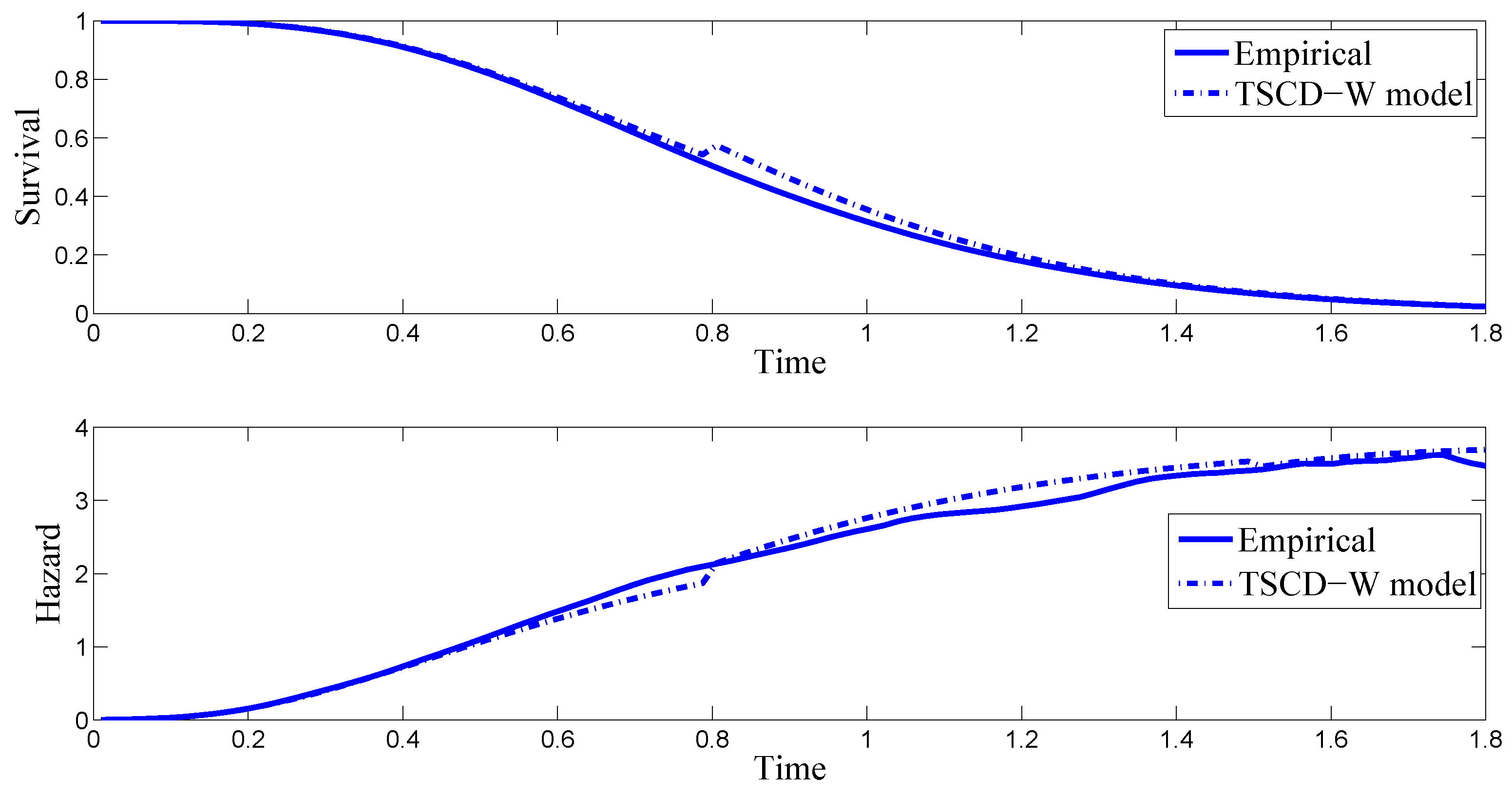
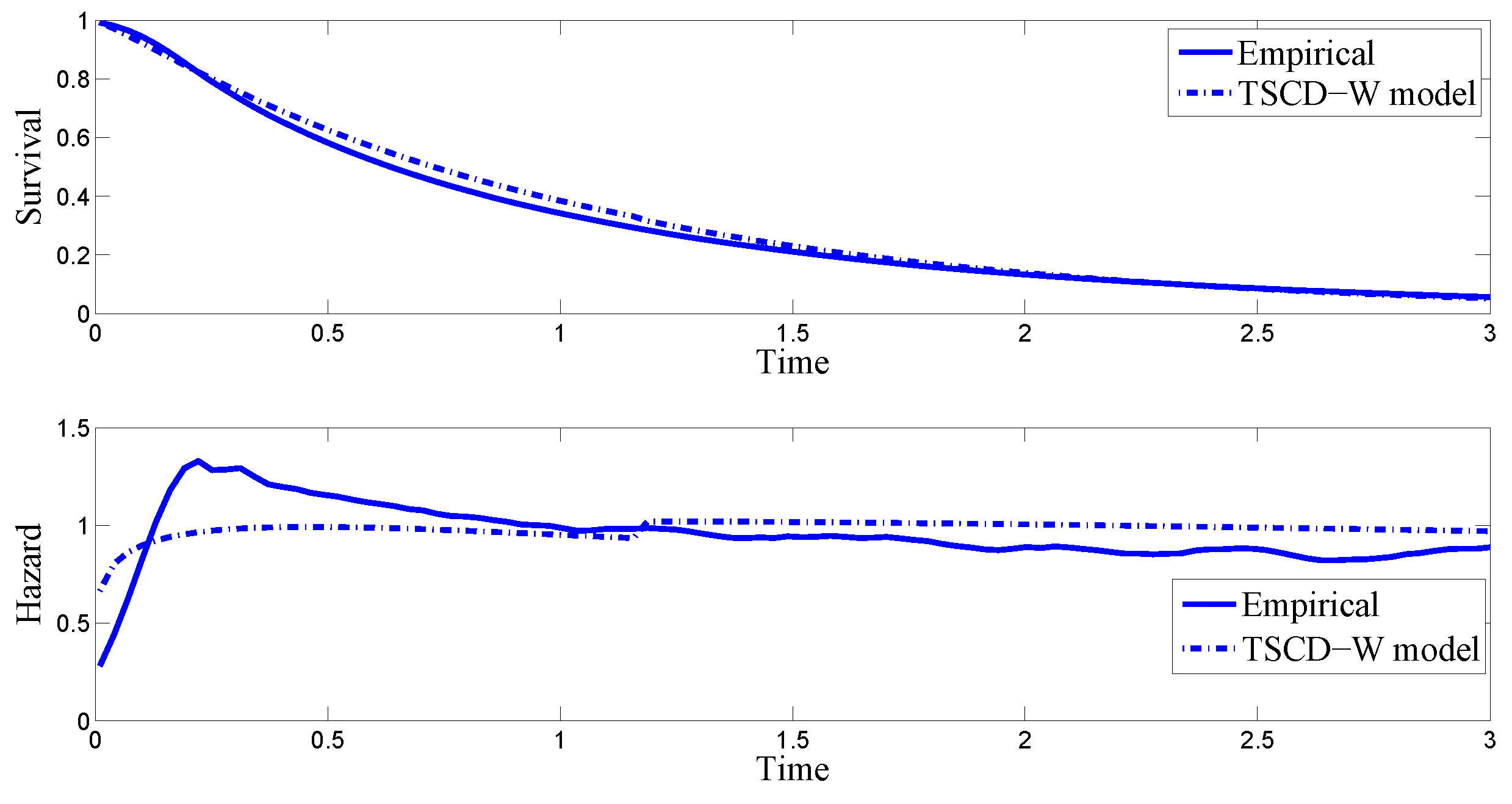
One way to assess the goodness-of-fit of the TSCD models is to compare the empirical survival function and the hazard function with those calculated from the fitted TSCD models visually. Denote by $f\left(y\right)$ and $F\left(y\right)=p(Y<y)$ respectively the pdf and cumulative distribution function (cdf) of the observed duration data. Then the survival function and the hazard function of the data are defined as $S\left(y\right)=1-F\left(y\right)$ and $H\left(y\right)=f\left(y\right)/(1-F(y\left)\right)$, respectively. As discussed in Bauwens and Veredas (2004), both the $f\left(y\right)$ and $F\left(y\right)$ for a given duration data have to be calculated by using a numerical method such as a kernel density fitting method, which can be found in Silverman (1986), pp. 11–13, and Bowman and Azzalini (1997). In addition, numerical integration methods such as the Gaussian quadrature method must be used for the calculation of $F\left(y\right)$ as well.

Given the highly comparable results reported in Table 1 for the Gamma and Weibull component cases, for brevity, we focus only on the Weibull component case in the subsequent discussion. The top panel in Figure 1 compares the empirical survival function of the simulated durations with the conditional survival function based on the TSCD-W model, while the bottom panel plots the corresponding empirical hazard of the simulated data together with the conditional hazard function. It is observed in the presented figures that the empirical survival function and the hazard function implied by the fitted TSCD-W model behave similarly to the empirical counterparts except that there is a very small jump at the threshold value of 0.7983. The reason for this jump is presumably because the threshold level of 0.8 was used in generating the artificial duration time series.

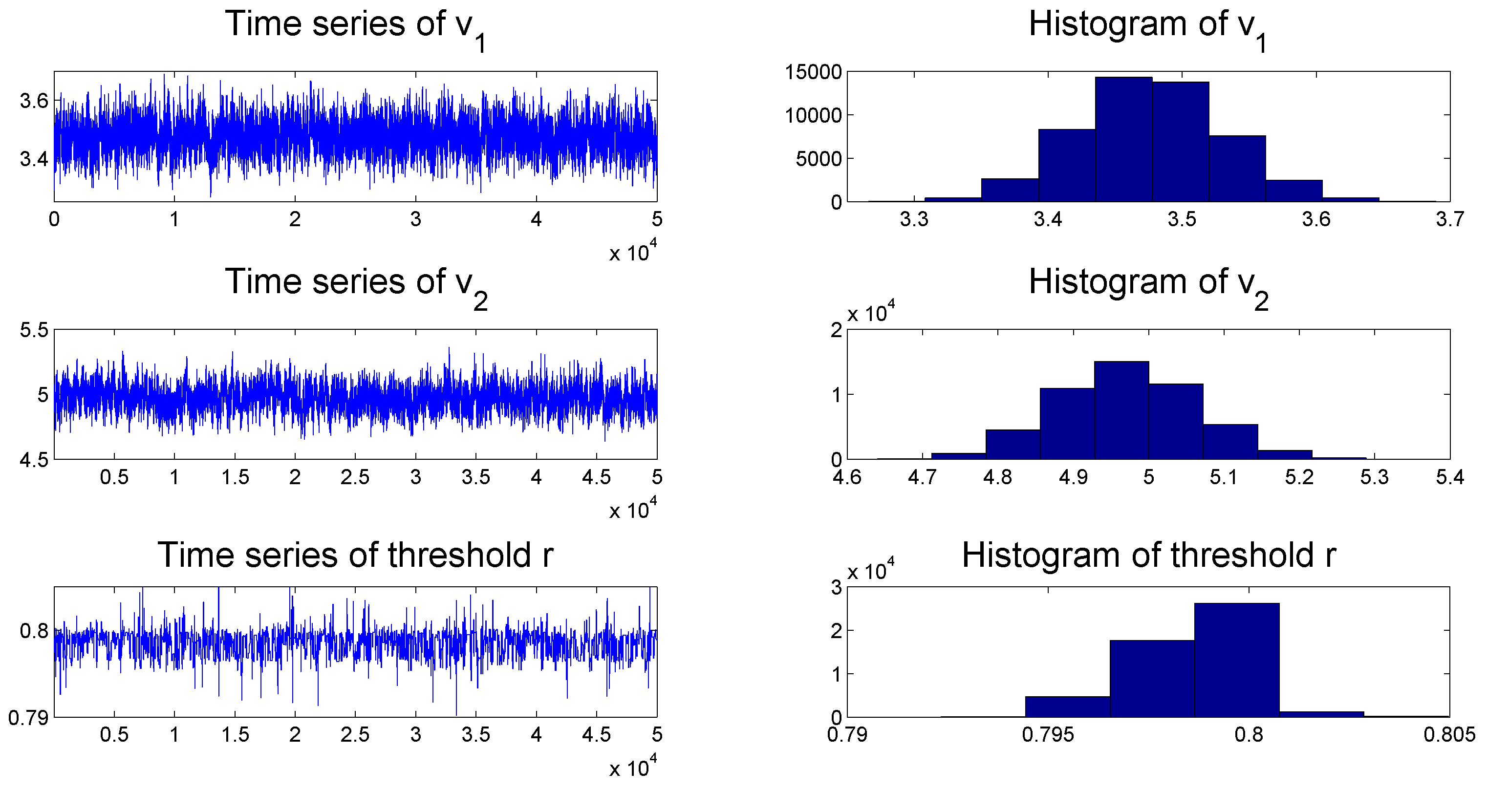
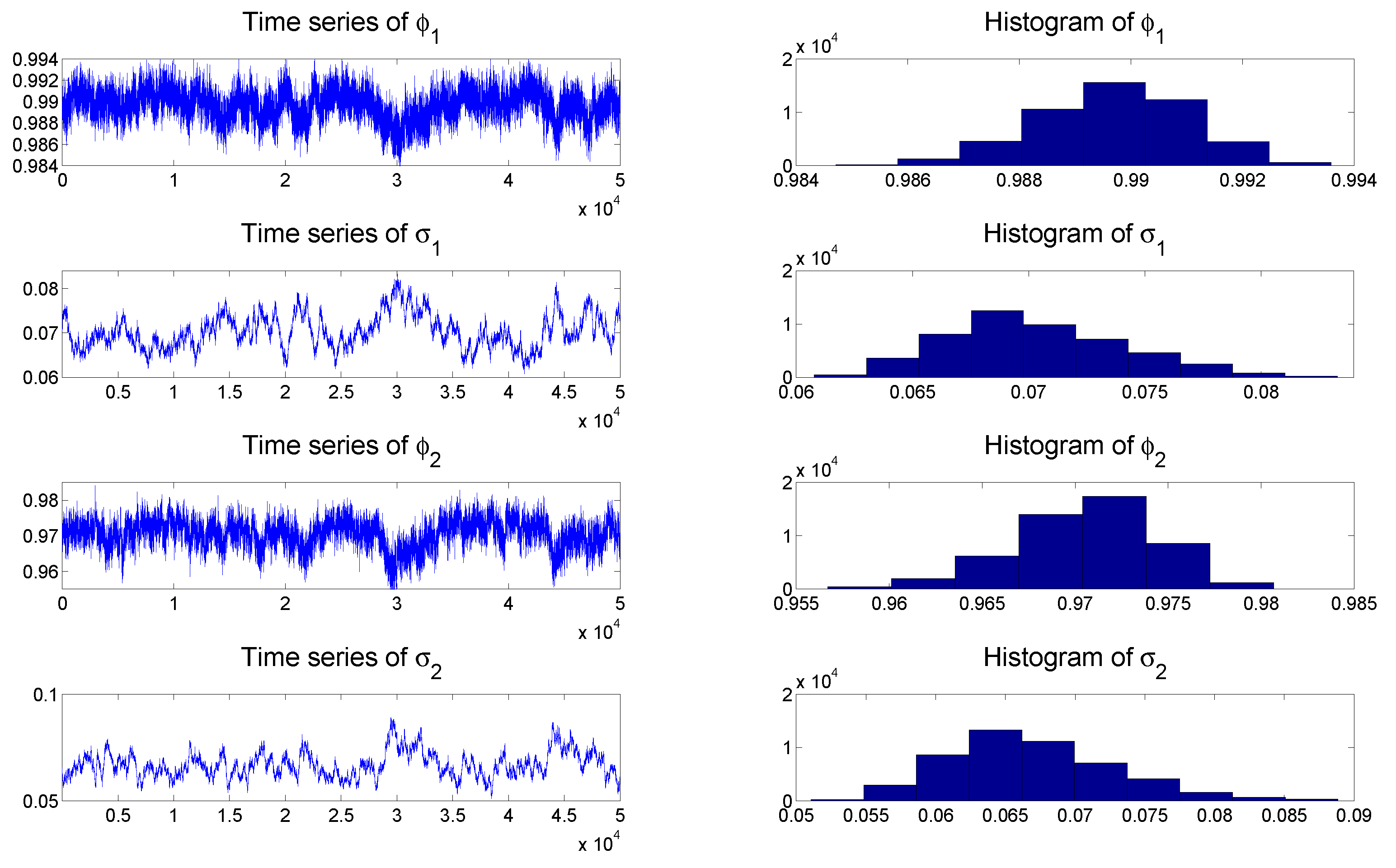
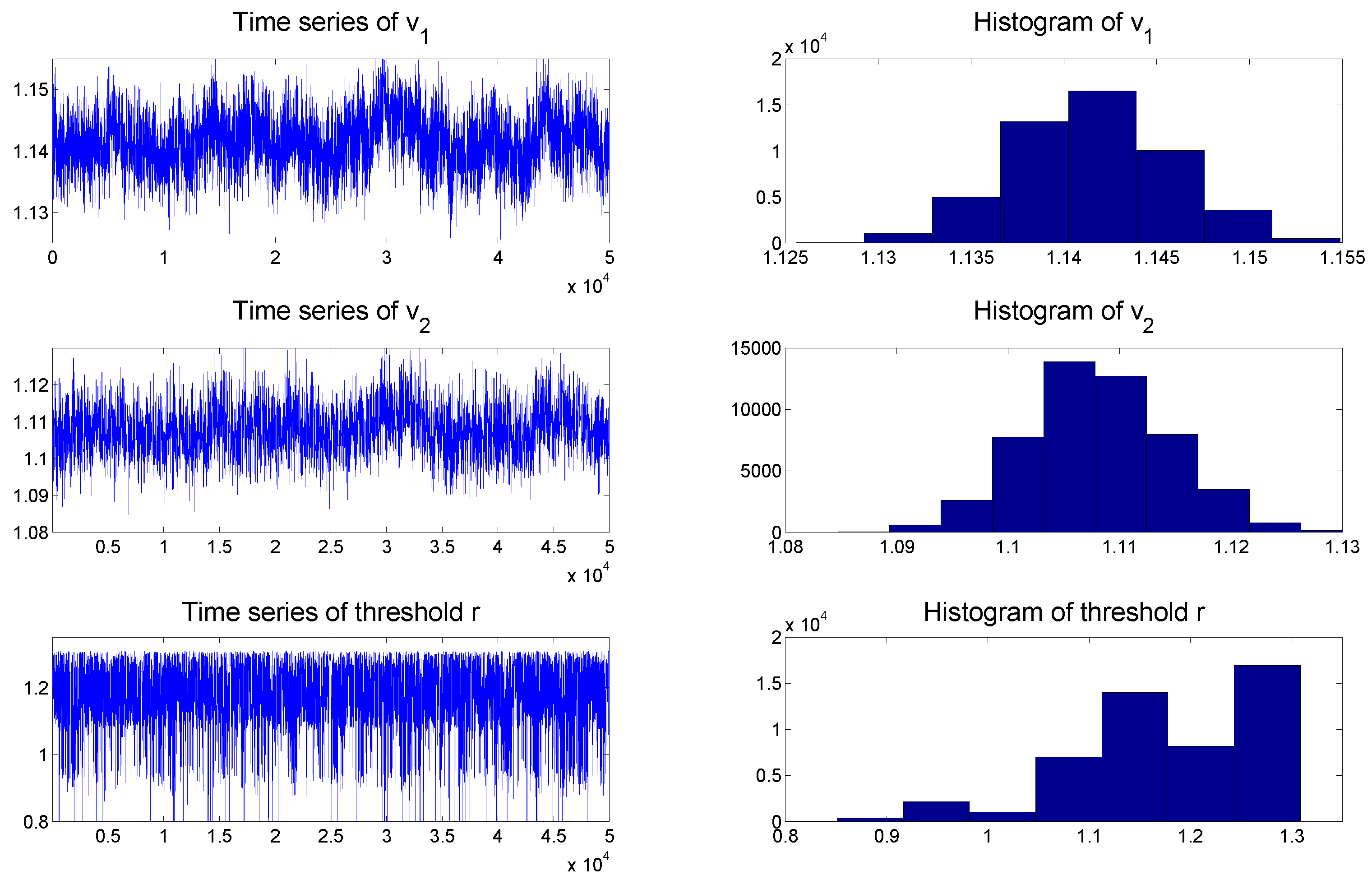
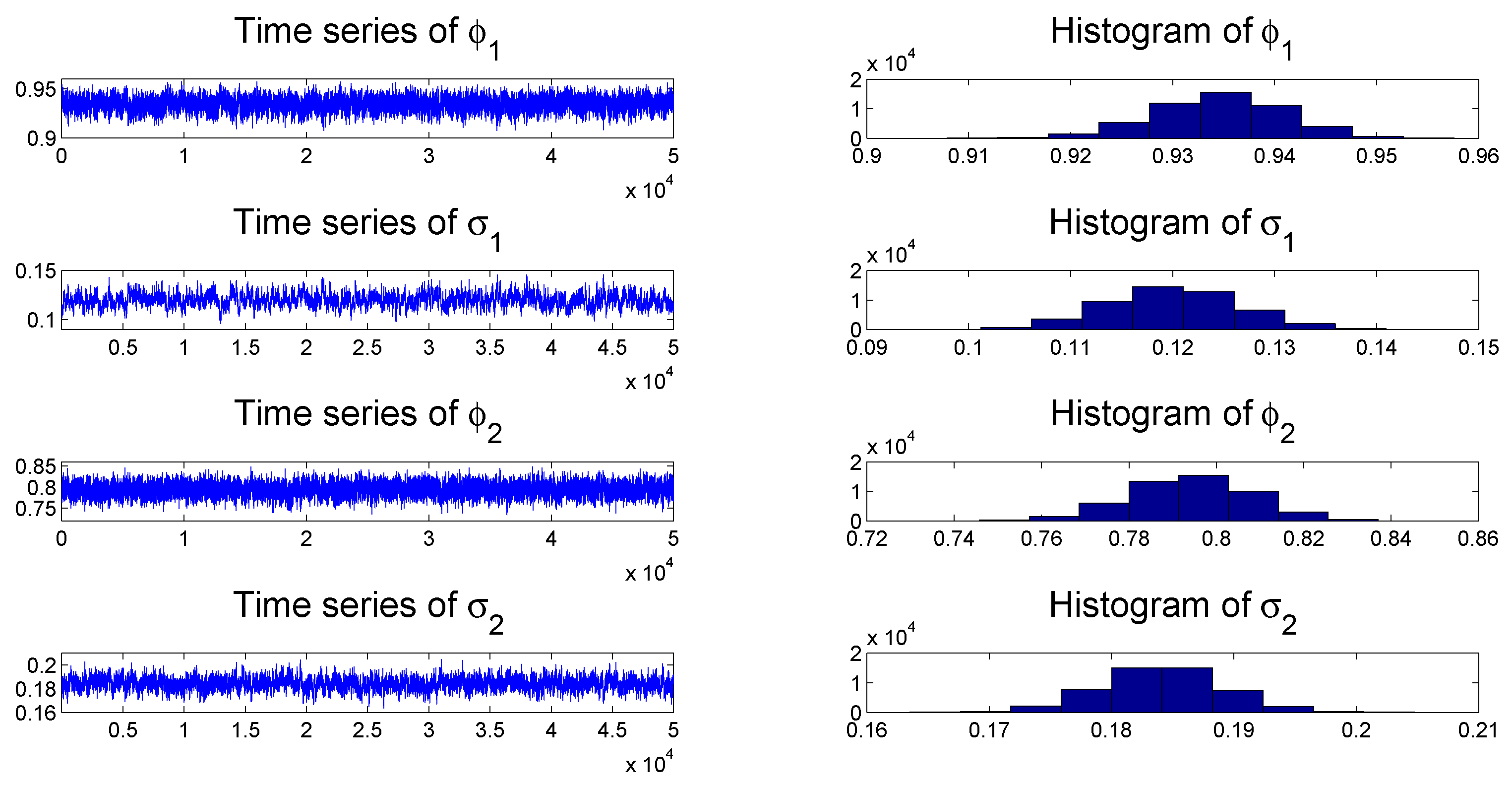
To check the convergence of the MCMC algorithms, we plot the histogram and time series of samples simulated from each posterior distribution of the parameters of the TSCD-W model in Figure 2 and Figure 3, respectively. It can be seen visually that the time series drawn from the full conditionals of parameters are convergent. Subsequent statistical tests also confirm this conclusion.

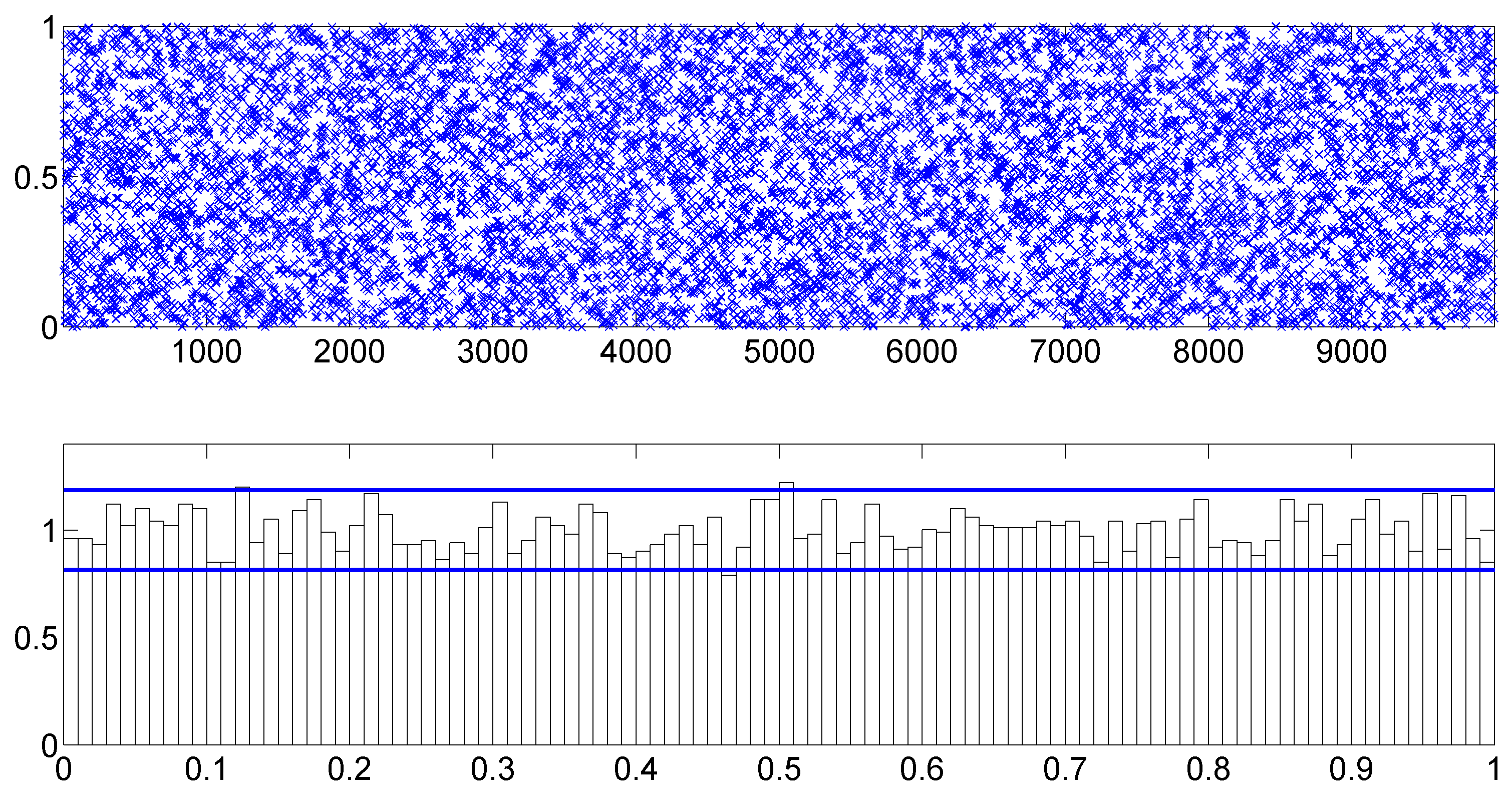
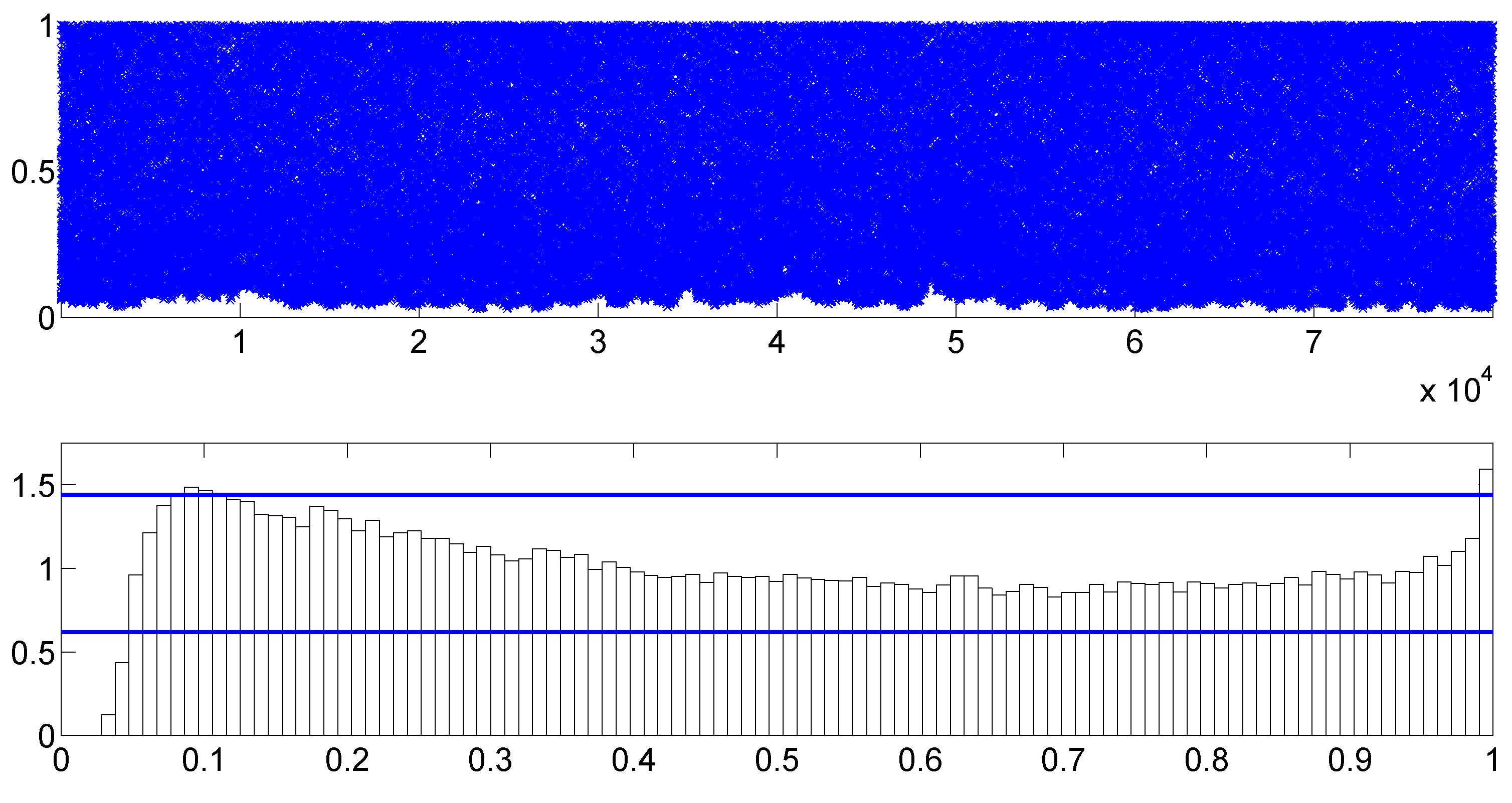
To assess the overall model fit, we consider the PITs calculated from the fitted TSCD-W model. Figure 4 includes the scatter and histogram plots of the PITs. The two horizontal lines in the histogram plot are the 95% confidence intervals of the uniformity, constructed under the normal approximation of a binomial distribution, the calculation of which is detailed in Diebold et al. (1998). It is evident that the PITs originated from the uniform distribution $U(0,1)$. The KS test statistic for the PITs is calculated as 0.0136 with the corresponding p-value of 0.8916. So, we do not reject the null hypothesis at any reasonable level of significance that the fitted TSCD model with the threshold Weibull innovations agrees with the generated duration data. 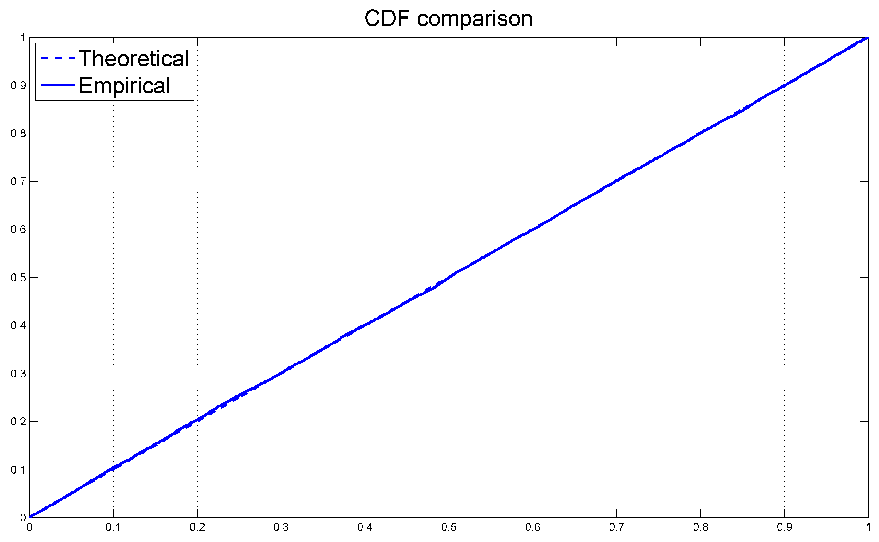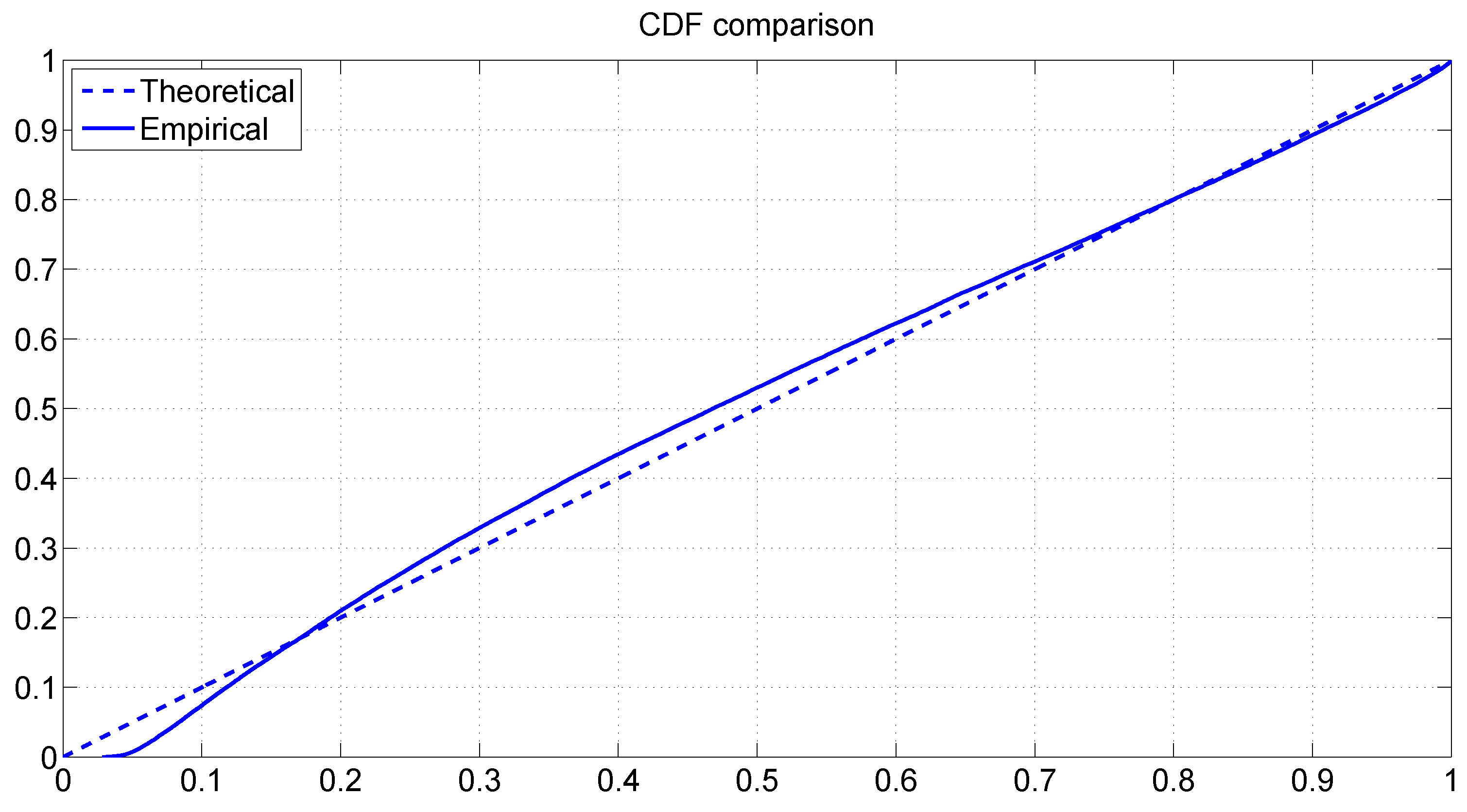Figure 5 graphs the cdf of the uniform distribution $U(0,1)$ together with the empirical cdf of the PITs. The two cdfs appear to be very close with each other, which confirms our earlier conclusion. 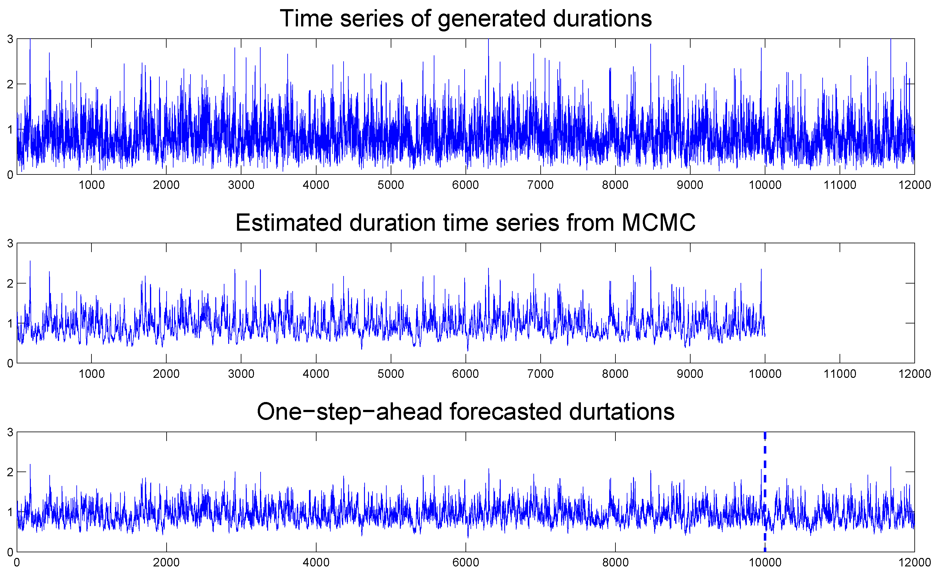Figure 6 compares the simulated durations with the filtered and one-step-ahead in-sample and out-of-sample forecasted durations, where the latter is separated by the vertical dotted line. We observe that the forecasted durations resemble the true durations, indicating that our TSCD-W model is again able to give a reasonably accurate forecast of future durations.

In applications to real data, although the true financial durations are not observable, we are reasonably confident that the fitted TSCD-W model can do a good job for duration forecast. While the above analysis is based on the TSCD-W model, we, unsurprisingly, also reach a very similar conclusion for the TSCD-G model.

Overall, the simulation studies carried out above demonstrate that the TSCD models and MCMC methods can recover the true parameters obtained by using the simulated duration data. In addition, duration forecasting can also be adequately performed using the AFP.

6. Empirical Analysis

In this section, we apply the proposed TSCD model to the classic/benchmark IBM and Boeing transaction data. Both data sets have been used previously in Knight and Ning (2008); Xu et al. (2011) and Men et al. (2015, 2016a). The IBM transaction data cover the period from 1 November 1990 to 31 January 1991 with a total of 24,765 transactions, while the Boeing data covers the period from 1 September 2001, to 31 October 2001 with a total of 90,136 observations. These datasets are admittedly from several decades ago. However, the use of these datasets is intended to facilitate a direct comparison between the results obtained from our models and methods with those in the literature (including our own previous studies), which all have conveniently used these same benchmark datasets. The frequency of the data is tick by tick, which records every single transaction that occurs in the market. Its salient feature is irregularly spaced in time and is primarily caused by financial transactions being clustered over time or occurring in a scattered fashion over time. The main implication of the irregular spacing of these data is that the time between any two consecutive market events, which is the financial duration, is a random variable.

Table 2. Parameter estimates based on TSCD models based on the IBM transaction data.

Parameter	Est.	Std.	HPD CI(95%)
Panel A: With Gamma($\gamma$,1) components
${\varphi }_1$	0.9704	0.0061	(0.9588, 0.9818)
${\sigma }_1$	0.1788	0.0129	(0.1538, 0.2037)
${\varphi }_2$	0.8065	0.0322	(0.7431, 0.8667)
${\sigma }_2$	0.2096	0.0254	(0.1618, 0.2593)
${\gamma }_1$	1.0015	0.0135	(0.9768, 1.0278)
${\gamma }_2$	0.9528	0.0120	(0.9287, 0.9767)
r	1.0337	0.2010	(0.7377, 1.3145)
Panel B: With Weibull(v,1) components
${\varphi }_1$	0.9847	0.0043	(0.9766, 0.9933)
${\sigma }_1$	0.1369	0.0090	(0.1180, 0.1535)
${\varphi }_2$	0.8640	0.0290	(0.8223, 0.9018)
${\sigma }_2$	0.1397	0.0144	(0.1114, 0.1681)
$v_1$	0.9664	0.0075	(0.9553, 0.9843)
$v_2$	0.9280	0.0101	(0.9001, 0.9393)
r	0.9622	0.1756	(0.6711, 1.2980)

and

Table 3. Parameter estimates based on TSCD models based on the Boeing transaction data.

Parameter	Est.	Std.	HPD CI(95%)
Panel A: With Gamma($\gamma$,1) components
${\varphi }_1$	0.9979	0.0012	(0.9956, 1.0000)
${\sigma }_1$	0.0573	0.0036	(0.0501, 0.0640)
${\varphi }_2$	0.9923	0.0020	(0.9897, 0.9951)
${\sigma }_2$	0.0496	0.0040	(0.0430, 0.0599)
${\gamma }_1$	1.2697	0.0097	(1.2506, 1.2891)
${\gamma }_2$	1.2959	0.0067	(1.2832, 1.3089)
r	0.3420	0.1363	(0.2778, 0.4682)
Panel B: With Weibull(v,1) components
${\varphi }_1$	0.9897	0.0014	(0.9869, 0.9923)
${\sigma }_1$	0.0703	0.0038	(0.0636, 0.0780)
${\varphi }_2$	0.9705	0.0039	(0.9626, 0.9778)
${\sigma }_2$	0.0669	0.0060	(0.0559, 0.0787)
$v_1$	1.1415	0.0043	(1.1332, 1.1499)
$v_2$	1.1081	0.0064	(1.0960, 1.1208)
r	1.1775	0.0974	(0.0965, 1.3085)

present the estimated parameters of the TSCD models based on the two data sets. The proposed MCMC algorithms were iterated 100,000 times. After the first 50,000 sampled values are discarded as the burn-in to eliminate initial value problems, the parameters and the states were then estimated by sample means. Standard errors and Bayesian HPD intervals are also reported in the two tables. The Bayesian HPD intervals are calculated by the $2.5\%$ and $97.5\%$ quartiles. The relatively small standard errors of these Bayesian HPD intervals indicate that our estimation process is quite efficient.

We note that for the IBM transaction data, the two persistent parameter estimates (e.g., for the TSCD-W model, $\widehat{{\varphi }_1}=0.9847$ and $\widehat{{\varphi }_2}=0.8640$) and, to a lesser extent, also the two volatility parameter estimates (e.g., for the TSCD-W model, $\widehat{{\sigma }_1}=0.1369$ and $\widehat{{\sigma }_2}=0.1397$) of the latent threshold AR(1) processes are quite different from each other. This indicates that at least two latent dynamic market factors that affect the duration innovation in different scales can be captured by the TSCD model. In other words, the IBM transaction data can be adequately characterized by the two specified threshold processes in the TSCD model. However, for the Boeing transaction data, the parameter estimates between the two regimes are relatively closer to each other (e.g., for the TSCD-W model, $\widehat{{\varphi }_1}=0.9897$ and $\widehat{{\varphi }_2}=0.9705$, and $\widehat{{\sigma }_1}=0.0703$ and $\widehat{{\sigma }_2}=0.0669$).

Again, given the highly comparable results for the Gamma and Weibull component cases for both datasets reported in Table 2 and Table 3, for brevity and without much loss of generality, we focus our ensuing discussion only for the Weibull component case, i.e., the TSCD-W model. However, the fitted TSCD-G model will later be subjected to a formal model discrimination against the fitted TSCD-W model for both datasets.

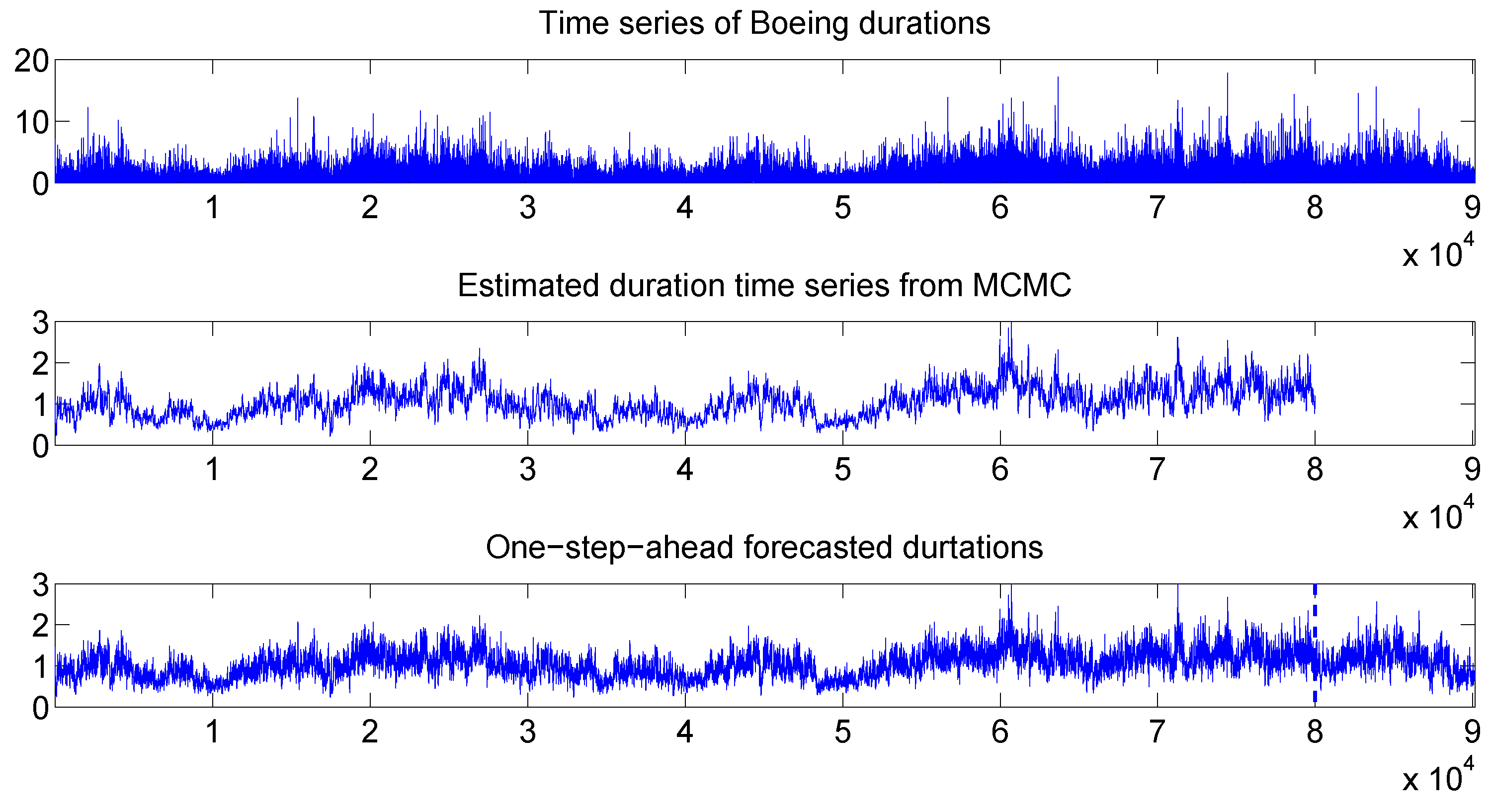
To check the convergence of the samples drawn from the full conditionals, we again plot the time series and histograms for each parameter of the TSCD-W models based on the Boeing transaction data in Figure 7 and Figure 8. It is visually evident that these time series are convergent. Please note that in our TSCD models, after 50,000 iterations, the generated time series typically converge. Figure 9 compares the duration time series with the filtered (or, Bayesian estimated) durations, and with the one-step-ahead in-sample and out-of-sample forecasted durations. It is observed that the forecasted durations also resemble the true durations closely.

As we did in the simulation studies, we compare in Figure 10 the empirical survival function of the Boeing durations with the conditional survival function based on the estimated TSCD-W model. The bottom panel plots the corresponding empirical hazard of the Boeing data together with the conditional hazard function. It is observed that the empirical survival function and the hazard function behave similarly to the counterparts implied by the fitted TSCD model except that there is a very small jump at the threshold value of 1.1775 in the hazard function implied by the fitted model.

To check the goodness-of-fit of the model, we plot the scatter and histogram plots of the PITs originated from the fitted TSCD-W model in Figure 11, while Figure 12 plots the empirical cdf of the PITs together with the theoretical cdf of the uniform distribution $U(0,1)$. The plots reveal that the PITs do not appear to follow a uniform distribution over the interval (0,1). The results from the KS test confirm this assertion. The reason for these unfavorable results can be understood by inspecting Figure 11 and Figure 12 where we see that the right tail of the marginal distribution of the data is well fitted, but the left tail of the marginal distribution is less so. The intensity of small durations is around 0.18. Bauwens and Veredas (2004); Feng et al. (2004) and Men et al. (2015, 2016a) also observed a similar lack of fit for their SCD models to duration data. Fractional latent processes have been proposed to improve the fit of the model. Distributional assumptions for the innovations of the duration equation other than the Gamma and Weibull distributions may also prove to be fruitful in this regard.3

Given the above qualification, we next proceed to select a better TSCD model for each of the two data sets of transactions by calculating the DIC values from the four fitted TSCD models. Berg et al. (2004) propose that the DIC be calculated by using the conditional likelihood. It is referred to as the conditional DIC. The conditional DIC is widely used for comparing SV models and is also used in the earlier version of this paper. In this paper, we follow Celeux et al. (2006) in computing the DIC by using an observed-data likelihood. This is referred to as an observed-data DIC. This observed-data DIC is not computed in practice due to the difficulty in evaluating the observed-data likelihood. However, despite its popularity, the Monte Carlo study reported by Chan and Grant (2016) shows that the conditional DIC tends to pick overfitted models (often with negative values of $p_D$, which is difficult to justify), whereas the observed-data DIC is better able to choose the correct model. The challenge associated with the computation of the observed-data DICs for the proposed TSCD models is overcome by suitably modifying importance sampling algorithms proposed by Chan and Grant (2016) for estimating the observed-data likelihoods for SV models.

The observed-data DIC measures are listed in

Table 4. Model selection by using the observed-data DIC criterion.

Data	Model	$\mathit{D}\left(\mathit{\theta }\right)$	${\mathit{P}}_{\mathit{D}}$	DIC
IBM	TSCD-G	35,960.8	14.4	35,975.2
	TSCD-W	36,305.7	19.6	36,325.3
Boeing	TSCD-G	146,155.6	15.4	146,171.0
	TSCD-W	147,022.5	20.1	147,042.6

. First, note that the computed values of $P_D$ for both models are positive, suggesting a positive penalty for model complexity, which makes sense. Second, for both the IBM and Boeing transaction data, the TSCD-G model is preferred given that the two fitted TSCD-G models have smaller observed-data DIC values compared to the TSCD-W counterparts.4

To undertake a further specification analysis, we pre-set ${\varphi }_1={\varphi }_2=\varphi$, and ${\sigma }_1={\sigma }_2=\sigma$ to arrive at a restricted TSCD (RTSCD) model.5 Thus, this RTSCD model is obtained by not allowing the latent first-order autoregressive process of the log conditional duration process to switch between the two regimes. However, it still permits the innovations of the duration process to follow a threshold distribution with a positive support. To select a better fitted RTSCD models for the IBM and Boeing transaction data, we compute the observed-data DICs from the models. The values of the observed-data DICs are presented in

Table 5. Restricted model selection by using the observed-data DIC criterion.

Data	Model	$\mathit{D}\left(\mathit{\theta }\right)$	${\mathit{P}}_{\mathit{D}}$	DIC
IBM	TSCD-G	35,981.9	10.7	35,992.6
	TSCD-W	36,378.2	12.5	36,390.7
Boeing	TSCD-G	146,182.3	11.9	146,194.2
	TSCD-W	147,064.6	16.3	147,080.9

. Among the observed-data DIC values, the smallest ones are from the RTSCD-G model, which means that the RTSCD-G model is better suited than the RTSCD-W model for the analysis of the real transaction data of the IBM and Boeing stocks.6 In addition, the computed DICs for the unrestricted TSCD models are uniformly smaller than those for the RSTCD models, suggesting that the unrestricted TSCD models are the preferred models for both datasets.7 Thus, for these datasets, the latent first-order autoregressive process of the log conditional duration process switch between the two regimes.

What is the economic interpretation of the findings in this paper? The findings are consistent with the prediction of the market micro-structure theory (MMT) in finance. The MMT suggests that there are informed and uninformed traders in the financial market. The interaction between the two trader types through information-revealing price formation processes is consistent with the observed financial market behavior. The informed traders will buy if the market price of an asset is below the true value (based on their information set). Conversely, they will sell, if the price is above the value. However, information is not free to the traders, and there are traders who base their trading decisions by observing the asset prices. As this latter trader type is a follower, its actions will be regulated by a distinct innovation process. This difference in behavior is consistent with the introduction of the two regimes for the innovation process in the TSCD model, since the instantaneous rate of transaction can be seen as being different across the two trader types.

7. Concluding Remarks

In this paper, we have proposed a TSCD model to analyze financial duration time series. The innovations of the duration process were assumed to follow a threshold distribution, where component distributions could be either a Gamma distribution or a Weibull distribution. In addition, we also assumed that the logarithm of the conditional durations followed a threshold latent AR(1) process. In the specified TSCD model, we allowed for the informed and uninformed traders in the market. Loosely speaking, these two types of traders have different trading behavior in response to the information arriving in the market. Suitable MCMC methods were developed for Bayesian inference of the parameters of the models in which the latent states were estimated as a by-product. Using the APF, the one-step-ahead in-sample and out-of-sample duration forecasts were carried out in a relatively straightforward way. Simulation studies and applications to two classic/benchmark data set of IBM and Boeing transactions demonstrated that the threshold SCD models work reasonably well in terms of parameter estimation and duration forecasting.

We have also considered a restricted version of the TSCD (RTSCD) model, in which the latent first-order autoregressive process of the log conditional duration process does not switch between the two regimes. We found that the RTSCD-G model performs better than the RTSCD-W model, when they are applied to both the IBM and Boeing transaction data. In addition, the proposed, unrestricted TSCD models uniformly outperform the restricted counterparts for both datasets.

Lastly, one important task remains outstanding at this juncture; i.e., we still need to further improve the empirical fit of the left tail of the marginal distribution of financial duration data. This entails a continued search for an ideal distribution of the financial duration data.

References

1. Akaike, Hirotugu. 1987. Factor Analysis and AIC. Psychometrika 52: 317–32. [Google Scholar] [CrossRef]
2. Bauwens, Luc, and David Veredas. 2004. The Stochastic Conditional Duration Model: A Latent Variable Model for the Analysis of Financial Durations. Journal of Econometrics 119: 381–482. [Google Scholar] [CrossRef]
3. Berg, Andreas, Renate Meyer, and Jun Yu. 2004. Deviance Information Criterion for Comparing Stochastic Volatility Models. Journal of Business and Economic Statistics 22: 107–20. [Google Scholar] [CrossRef]
4. Bowman, Adrian W., and Adelchi Azzalini. 1997. Applied Smoothing Techniques for Data Analysis. New York: Oxford University Press. [Google Scholar]
5. Celeux, Gilles, Florence Forbes, Christian P. Robert, and D. Mike Titterington. 2006. Deviance information criteria for missing data models. Bayesian Analysis 1: 651–74. [Google Scholar] [CrossRef]
6. Chan, Joshua C. C., and Angelia L. Grant. 2016. On the Observed-Data Deviance Information Criterion for Volatility Modeling. Journal of Financial Econometrics 14: 772–802. [Google Scholar] [CrossRef]
7. Chib, Siddhartha, Federico Nardari, and Neil Shephard. 2006. Analysis of High Dimensional Multivariate Stochastic Volatility Models. Journal of Econometrics 134: 341–71. [Google Scholar] [CrossRef]
8. De Luca, Giovanni, and Giampiero M. Gallo. 2004. Mixture Processes for Financial Intradaily Durations. Studies in Nonlinear Dynamics & Econometrics 8: 1–12. [Google Scholar]
9. De Luca, Giovanni, and Giampiero M. Gallo. 2009. Time-Varying Mixing Weights in Mixture Autoregressive Conditional Duration Models. Econometric Reviews 28: 102–20. [Google Scholar] [CrossRef]
10. Diebold, Francis X., Todd A. Gunther, and Anthony S. Tay. 1998. Evaluating Density Forecasts with Applications to Financial Risk Management. International Economic Review 39: 863–83. [Google Scholar] [CrossRef]
11. Feng, Dingan, George J. Jiang, and Peter X. K. Song. 2004. Stochastic Conditional Duration Models with “Leverage Effect” for Financial Transaction Data. Journal of Financial Econometrics 2: 390–421. [Google Scholar] [CrossRef]
12. Jacquier, E., N. G. Polson, and P. E. Rossi. 2004. Bayesian Analysis of Stochastic Volatility Models with Fat-tails and Correlated Errors. Journal of Econometrics 122: 185–212. [Google Scholar] [CrossRef]
13. Knight, John L., and Cathy Q. Ning. 2008. Estimation of the Stochastic Conditional Duration Model via Alternative Methods. Econometrics Journal 11: 573–92. [Google Scholar] [CrossRef]
14. Lopes, Hedibert Freitas, and Mike West. 2004. Bayesian Model Assessment in Factor Analysis. Statistica Sinica 14: 41–67. [Google Scholar]
15. Men, Zhongxian, Tony S. Wirjanto, and Adam W. Kolkiewicz. 2013. A Threshold Stochastic Conditional Duration Model for Financial Transaction Data. Working Paper. Rimini Centre for Economic Analysis, pp. 30–13. Available online: http://www.rcea.org/RePEc/pdf/wp3013.pdf/ (accessed on 8 May 2019).
16. Men, Zhongxian, Tony S. Wirjanto, and Adam W. Kolkiewicz. 2014. A Threshold Stochastic Conditional Duration Model for Financial Transaction Data. Available online: https://ssrn.com/abstract=2241190 (accessed on 8 May 2019).
17. Men, Zhongxian, Adam W. Kolkiewicz, and Tony S. Wirjanto. 2015. Bayesian Analysis of Asymmetric Stochastic Conditional Duration Models. Journal of Forecasting 34: 36–56. [Google Scholar] [CrossRef]
18. Men, Zhongxian, Adam W. Kolkiewicz, and Tony S. Wirjanto. 2016a. Bayesian Inference of Asymmetric Stochastic Conditional Duration Models. Journal of Statistical Computation and Simulation 86: 1295–1319. [Google Scholar] [CrossRef]
19. Men, Zhongxian, Don McLeish, Adam W. Kolkiewicz, and Tony S. Wirjanto. 2016b. Comparison of Asymmetric Stochastic Volatility Models under Different Correlation Structures. Journal of Applied Statistics 44: 1350–68. [Google Scholar] [CrossRef]
20. Men, Zhongxian, Tony S. Wirjanto, and Adam W. Kolkiewicz. 2019. Threshold Model for Financial Duration Data. Unpblished Working Paper. Waterloo: University of Waterloo. [Google Scholar]
21. Mira, Antonietta, and Luke Tierney. 2002. Efficiency and Convergence Properties of Slice Samplers. Scandinavian Journal of Statistics 29: 1–12. [Google Scholar] [CrossRef]
22. Neal, Radford M. 2003. Slice Sampling. The Annals of Statistics 31: 705–67. [Google Scholar] [CrossRef]
23. Pitt, Michael K., and Neil Shephard. 1999. Filtering via Simulation: Auxiliary Particle Filters. Journal of the American Statistical Association 94: 590–99. [Google Scholar] [CrossRef]
24. Roberts, G. O., and J. S. Rosenthal. 1999. Convergence of Slice Sampler Markov Chains. Journal of the Royal Statistical Society Series B (Statistical Methodology) 61: 643–60. [Google Scholar] [CrossRef]
25. Schwarz, Gideon. 1978. Estimating the Dimension of a Model. Annals of Statistics 6: 461–64. [Google Scholar] [CrossRef]
26. Silverman, Bernard. W. 1986. Density Estimation for Statistics and Data Analysis. London: Chapman & Hall. [Google Scholar]
27. Spiegelhalter, David J., Nicola G. Best, Bradley P. Carlin, and Angelika van der Linde. 2002. Bayesian Measures of Model Complexity and Fit (with discussion). Journal of the Royal Statistical Society, Series B 64: 583–639. [Google Scholar] [CrossRef]
28. Xu, Dinghai, John Knight, and Tony S. Wirjanto. 2011. Asymmetric Stochastic Conditional Duration Model—A Mixture-of-Normal Approach. Journal of Financial Econometrics 9: 469–88. [Google Scholar] [CrossRef]
29. Yu, Jun, Zhenlin Yang, and Xibin Zhang. 2006. A class of nonlinear stochastic volatility models and its implication for pricing currency options. Computational Statistics and Data Analysis 51: 2218–31. [Google Scholar] [CrossRef]
30. Zhang, Xibin, and Maxwell L. King. 2008. Box-Cox Stochastic Volatility Models with Heavy-tails and Correlated Errors. Journal of Empirical Finance 15: 549–66. [Google Scholar] [CrossRef]
1
This paper is built from materials presented in several earlier working papers by the authors in Men et al. (2013, 2014, 2019).
2
For further efficiency considerations, Pitt and Shephard (1999) for instance proposes the use of block samplers for h t for a stochastic volatility (SV) model. We have tried to apply this block sampling scheme to our variant of the TSCD models and found the required computation to be highly intractable.
3
Another potential source of rejection for the KS statistic may lie in the fact that it is calculated by using estimated parameters in the empirical analysis. This alters the standard limiting distribution of the KS statistics to a non-standard one involving functionals of Brownian bridges.
4
The conditional DICs for the TSCD-G model and the TSCD-W model are 35,669.5 and 36,025.1 for the IBM dataset and 145,874.4 and 146,749.1 for the Boeing dataset respectively. These results are comparable with those reported for the unobserved-data DICs.
5
We thank one of the anonymous reviewers for this suggestion.
6
The conditional DICs for the RTSCD-G model and the RTSCD-W model are 33,252.8 and 33,557.9 for the IBM dataset and 143,287.3 and 144,758.8 for the Boeing dataset respectively. These results are comparable with those reported for the unobserved-data DICs but in all four cases the effective numbers of parameters, P D , are negative, implying a negative penalty for model complexity, which is difficult to justify.
7
The conditional DICs for the RTSCD models are always smaller than those for the unrestricted TSCD models. This is because the effective number of parameters that measures the model complexity is positive in the observed-data DIC, which is expected, and negative in the conditional DIC, which is less plausible. This is consistent with the Monte Carlo study in Chan and Grant (2016). At the same time, the posterior mean deviance, which is used as a Bayesian measure of the model fit, is always negative in both methods.
Figure 1. Top Panel: conditional survival function of the TSCD-W model for the simulated durations and its empirical survival function. Bottom Panel: the corresponding conditional hazard function for the simulated data and its empirical hazard rate.
Jrfm 12 00088 g001
Figure 2. Time series and histograms of the samples drawn from the full conditionals of the parameters in the AR(1) process of the TSCD-W model based on the simulated duration data.
Jrfm 12 00088 g002
Figure 3. Time series and histograms of the samples drawn from the full conditionals of the parameters in the Weibull component distributions of the TSCD model and the full conditional of threshold based on simulated duration data.
Jrfm 12 00088 g003
Figure 4. Goodness-of-fit test via the scatter plot (top) and the histogram (bottom) of the PITs produced by the fitted TSCD-W model based on simulated transaction data. The two horizontal lines in the histogram plot are the 95% confidence intervals of the uniformity, constructed under the normal approximation of a binomial distribution, the calculation of which is detailed in Diebold et al. (1998).
Jrfm 12 00088 g004
Figure 5. Comparison between the empirical CDF of the PITs and the theoretical CDF of a uniform distribution over the interval [0, 1] based on the TSCD-W model using simulated transaction data.
Jrfm 12 00088 g005
Figure 6. Comparison between observed durations with the estimated and one-step-ahead forecasted conditional durations based on the TSCD-W model using the simulated transaction data.
Jrfm 12 00088 g006
Figure 7. Time series and histograms of the samples drawn from the full conditionals of the parameters in the AR(1) process of the double TSCD-W model based on the Boeing stock duration data.
Jrfm 12 00088 g007
Figure 8. Time series and histograms of the samples drawn from the full conditionals of the parameters of the TSCD-W model based on the Boeing duration data.
Jrfm 12 00088 g008
Figure 9. Comparison between observed durations, estimated, and one-step-ahead forecasted conditional durations based on the TSCD-W model using the Boeing stock transaction data.
Jrfm 12 00088 g009
Figure 10. Top Panel: conditional survival function of the TSCD-W model for the Boeing durations and its empirical survival function. Bottom Panel: the corresponding conditional hazard function for the Boeing durations data and its empirical hazard rate.
Jrfm 12 00088 g010
Figure 11. Scatter plot (top) and the histogram (bottom) of the PITs produced by the fitted TSCD-W model to the Boeing transaction data. The two horizontal lines in the histogram plot are the 95% confidence intervals of the uniformity, constructed under the normal approximation of a binomial distribution, the calculation of which is detailed in Diebold et al. (1998).
Jrfm 12 00088 g011
Figure 12. Comparison between the empirical CDF of the PITs and the theoretical CDF of a uniform distribution over the interval (0,1) based on the TSCD-W model to the Boeing transaction data.
Jrfm 12 00088 g012