Managerial Self-Attribution Bias and Banks’ Future Performance: Evidence from Emerging Economies


Abstract
1. Introduction
2. Literature Review
3. Methodology
3.1. Data
3.2. Variables and Their Definitions
3.2.1. Bank Performance Indicator
3.2.2. Performance Determinants
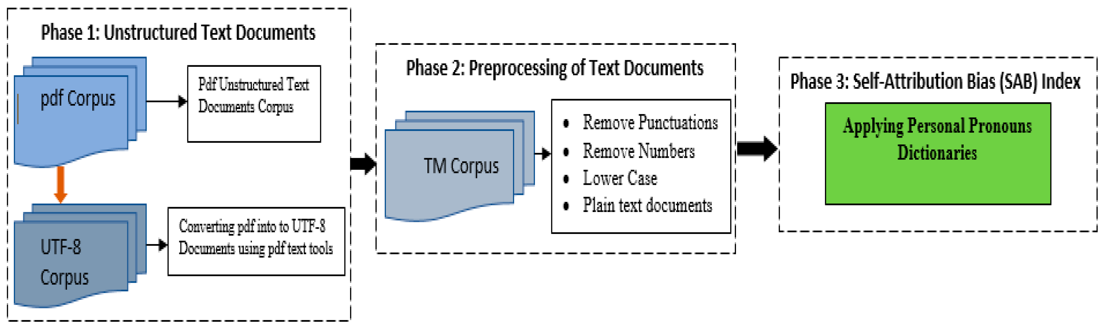
3.3. Measurement of Managerial Self-Attribution Bias
3.4. Econometric Model Using System GMM
Diagnostic Checks
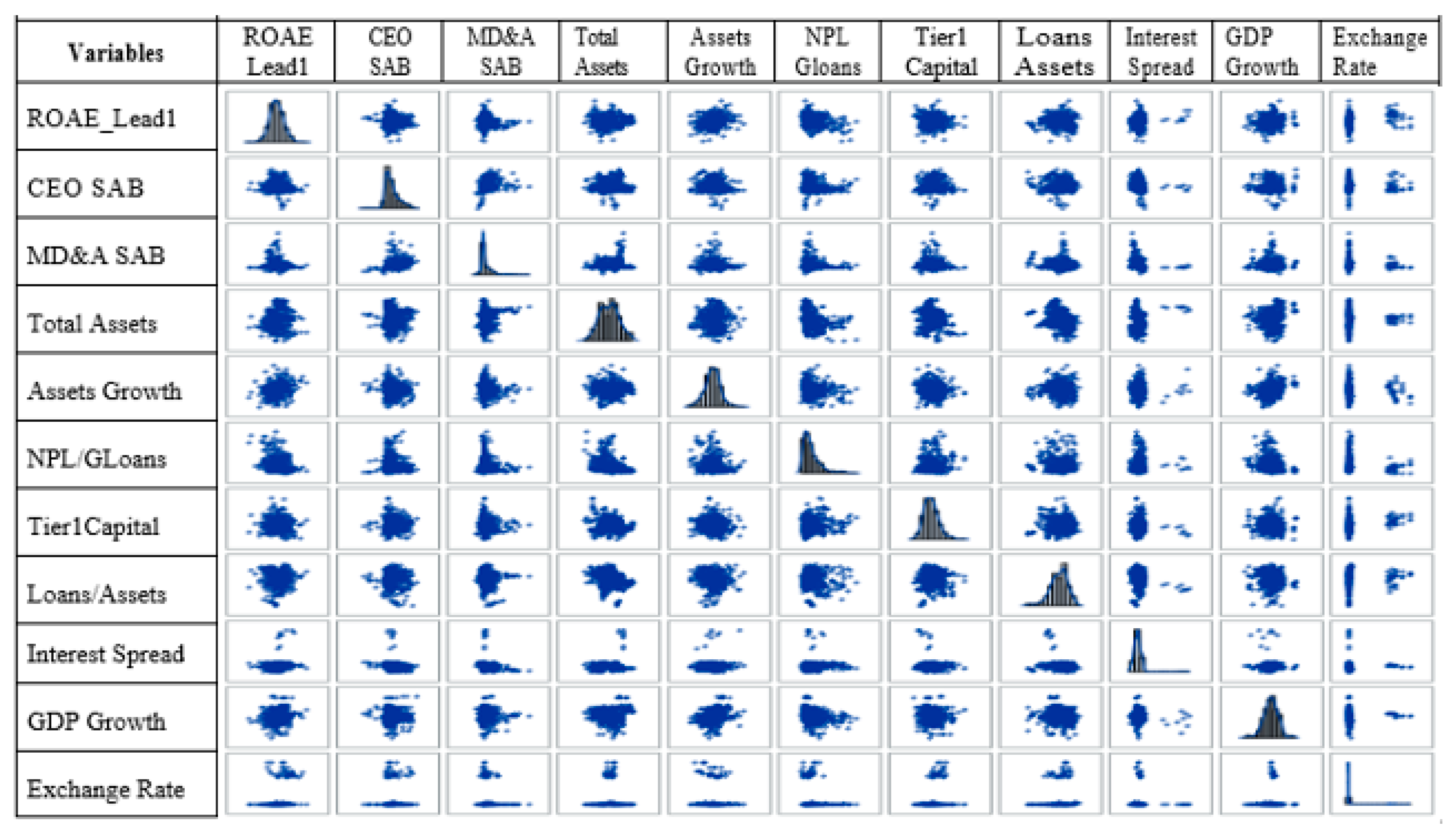
4. Descriptive Statistics
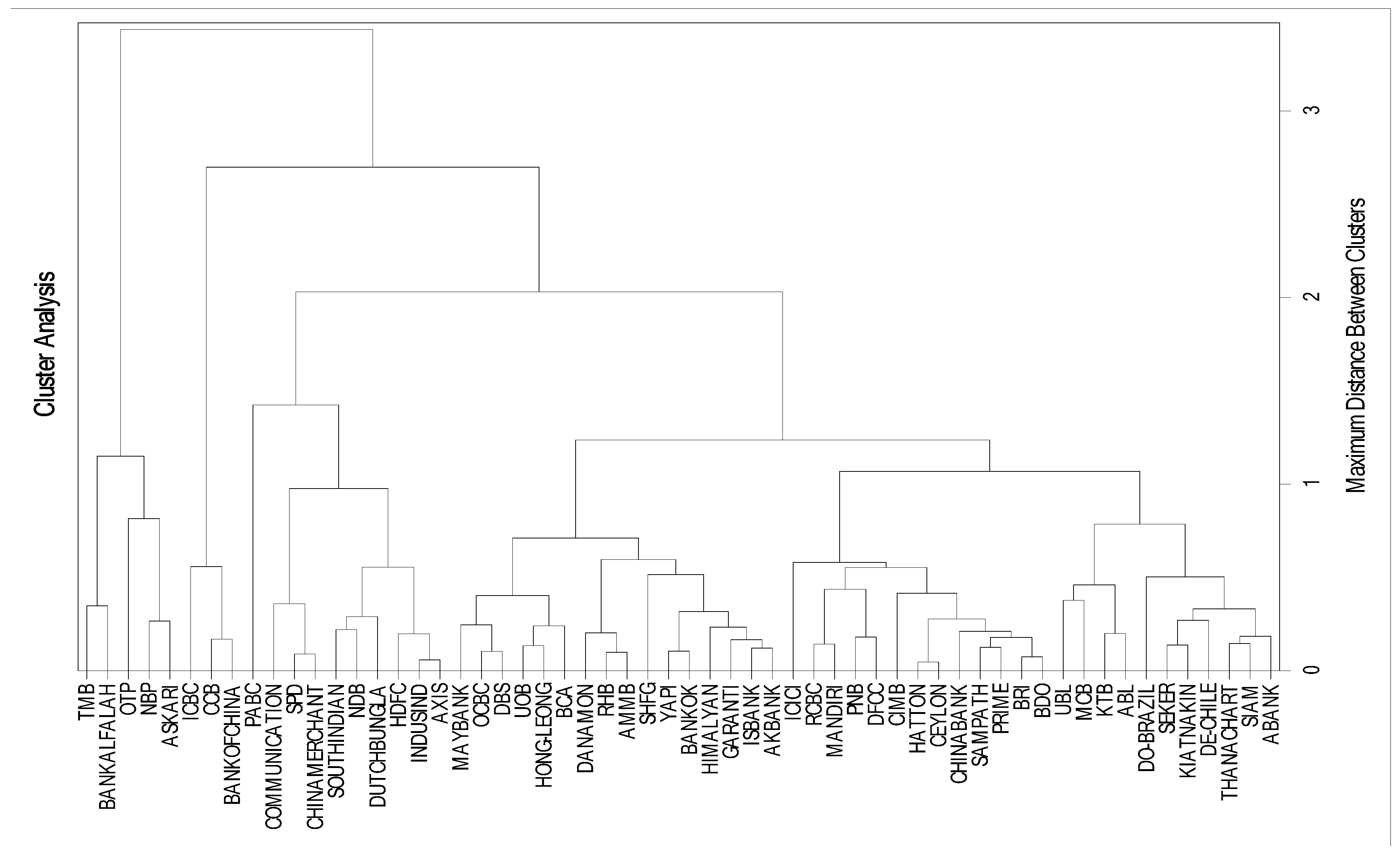
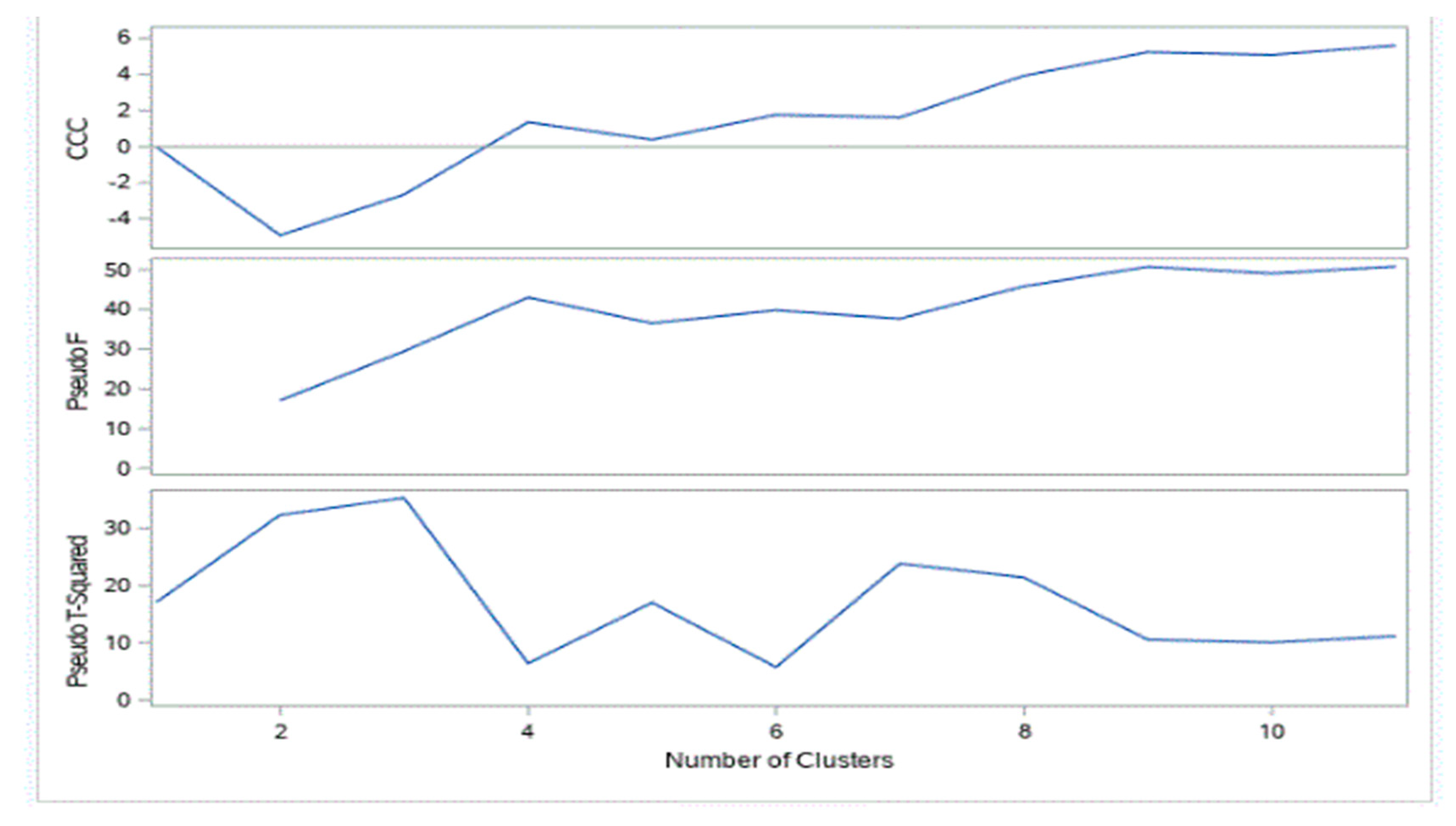
5. Agglomerative Hierarchical Clustering Analysis
5.1. Measurement of Distance between Observations
5.2. Cluster Profile
6. Econometric Analysis
6.1. Pre-Diagnostics Checks
6.2. Post Diagnostics Checks
6.3. Discussions
7. Conclusions
7.1. Policy Implications
7.2. Limitation of the Study
Author Contributions
Funding
Acknowledgments
Conflicts of Interest
Appendix A. List of Banks in Sample
| Country | Bank Name | Country | Bank Name |
| Bangladesh | Dutch Bungla Bank | Singapore | DBS |
| Prime Bank | OCBC | ||
| Brazil | Do-Brazil Bank | UOB | |
| Chile | De-Chile | Sri Lanka | Ceylon Bank |
| China | Bank of China | DFCC Bank | |
| CCB | Hatton Bank | ||
| China Merchant Bank | NDB Bank | ||
| Communication bank | PABC Bank | ||
| ICBC | Sampath Bank | ||
| SPD Bank | Thailand | Bangkok Bank | |
| Hungary | OTP Bank | Kiatnakin | |
| India | Axis Bank | KTB Bank | |
| HDFC | Siam Bank | ||
| ICICI Bank | Thana Chart Bank | ||
| Indusind Bank | TMB Bank | ||
| South Indian Bank | Turkey | ABank | |
| Indonesia | BCA Bank | AKBank | |
| BRI Bank | Garanti Bank | ||
| Danamon Bank | ISBank | ||
| Mandiri Bank | Seker Bank | ||
| Korea | SHFG Bank | Yapi | |
| Malaysia | AMMB Bank | ||
| CIMB Bank | |||
| Hong-Leong | |||
| May Bank | |||
| RHB Bank | |||
| Nepal | Himalayan Bank | ||
| Pakistan | ABL Bank | ||
| Askari Bank | |||
| Bank Alfalah | |||
| MCB | |||
| NBP | |||
| UBL | |||
| Philippines | BDO Bank | ||
| China Bank | |||
| PNB | |||
| RCBC Bank |
Appendix B. Descriptive Statistics by Country
| Country | N Obs | Variable | Mean | Median | Minimum | Maximum | CV | Std Dev |
| Bangladesh | 18 | ROAE_LEAD1 | 19.75 | 19.71 | 8.45 | 35.33 | 4.40 | 8.77 |
| CEO SAB | 28.94 | 28.50 | 8.00 | 57.00 | 48.26 | 3.97 | ||
| MD&A SAB | 23.72 | 25.00 | −17.00 | 58.00 | 93.34 | 22.14 | ||
| Total Assets | 2084.23 | 2058.43 | 719.95 | 3288.66 | 41.15 | 857.72 | ||
| Assets Growth | 14.11 | 15.39 | −4.85 | 26.42 | 60.42 | 8.53 | ||
| NPL/GLoans | 3.19 | 2.82 | 1.15 | 7.67 | 57.97 | 1.85 | ||
| Tier1Capital | 8.64 | 9.44 | 4.65 | 10.95 | 21.20 | 1.83 | ||
| Loans/Assets | 66.57 | 66.19 | 59.63 | 77.61 | 8.39 | 5.58 | ||
| Interest Spread | 4.24 | 4.48 | 1.87 | 5.64 | 29.24 | 1.24 | ||
| GDP Growth | 6.14 | 6.06 | 5.05 | 7.06 | 9.37 | 0.58 | ||
| Exchange Rate | 73.98 | 74.15 | 68.60 | 81.86 | 6.66 | 4.93 | ||
| Brazil | 9 | ROAE_LEAD1 | 20.72 | 18.41 | 15.44 | 29.61 | 25.26 | 5.23 |
| CEO SAB | 34.89 | 39.00 | 12.00 | 52.00 | 41.52 | 14.49 | ||
| MD&A SAB | 17.00 | 4.00 | 3.00 | 67.00 | 142.58 | 24.24 | ||
| Total Assets | 426,310.40 | 481,190.04 | 200,340.00 | 554,609.90 | 30.44 | 129,776.38 | ||
| Assets Growth | 9.70 | 7.61 | −12.33 | 46.31 | 169.32 | 16.43 | ||
| NPL/GLoans | 4.48 | 4.17 | 2.30 | 8.61 | 51.63 | 2.31 | ||
| Tier1Capital | 8.83 | 8.84 | 5.83 | 11.39 | 24.74 | 2.18 | ||
| Loans/Assets | 45.15 | 43.13 | 40.38 | 50.90 | 9.24 | 4.17 | ||
| Interest Spread | 29.97 | 31.34 | 19.58 | 35.59 | 18.87 | 5.66 | ||
| GDP Growth | 2.69 | 3.00 | −3.77 | 7.53 | 129.89 | 3.49 | ||
| Exchange Rate | 2.11 | 1.95 | 1.67 | 3.33 | 23.72 | 0.50 | ||
| Chile | 9 | ROAE_LEAD1 | 22.50 | 22.48 | 18.61 | 27.11 | 12.11 | 2.72 |
| CEO SAB | 53.89 | 57.00 | 26.00 | 82.00 | 30.79 | 16.59 | ||
| MD&A SAB | 121.44 | 133.00 | 45.00 | 182.00 | 43.98 | 53.41 | ||
| Total Assets | 29,227.61 | 21,741.00 | 12,583.00 | 49,514.80 | 49.27 | 14,399.67 | ||
| Assets Growth | 12.81 | 12.77 | −8.78 | 38.98 | 132.54 | 16.98 | ||
| NPL/GLoans | 5.02 | 3.53 | 1.34 | 9.92 | 62.91 | 3.16 | ||
| Tier1Capital | 10.03 | 8.92 | 7.25 | 13.32 | 24.38 | 2.45 | ||
| Loans/Assets | 79.00 | 79.13 | 75.29 | 83.06 | 3.08 | 2.44 | ||
| Interest Spread | 3.91 | 4.09 | 1.91 | 5.77 | 29.88 | 1.17 | ||
| GDP Growth | 3.63 | 3.98 | −1.04 | 5.84 | 63.14 | 2.29 | ||
| Exchange Rate | 533.99 | 522.46 | 483.67 | 654.12 | 10.17 | 54.31 | ||
| China | 54 | ROAE_LEAD1 | 19.31 | 19.84 | 11.71 | 27.90 | 17.44 | 3.37 |
| CEO SAB | 17.87 | 8.00 | −3.00) | 123.00 | 124.97 | 22.33 | ||
| MD&A SAB | 14.00 | 2.00 | −19.00) | 100.00 | 209.31 | 29.30 | ||
| Total Assets | 1,285,860.17 | 996,974.44 | 153,270.17 | 3,421,363.16 | 72.79 | 936,017.03 | ||
| Assets Growth | 15.75 | 16.78 | 1.55 | 33.35 | 40.78 | 6.42 | ||
| NPL/GLoans | 1.40 | 1.13 | 0.44 | 3.17 | 51.05 | 0.72 | ||
| Tier1Capital | 9.81 | 10.08 | 4.02 | 13.48 | 18.03 | 1.77 | ||
| Loans/Assets | 52.78 | 53.27 | 44.52 | 59.58 | 6.38 | 3.37 | ||
| Interest Spread | 3.03 | 3.06 | 2.85 | 3.33 | 4.44 | 0.13 | ||
| GDP Growth | 9.26 | 9.40 | 6.92 | 14.23 | 23.10 | 2.14 | ||
| Exchange Rate | 6.61 | 6.46 | 6.14 | 7.61 | 6.90 | 0.46 | ||
| Hungary | 9 | ROAE_LEAD1 | 9.07 | 8.36 | −7.37 | 26.25 | 101.55 | 9.22 |
| CEO SAB | 38.56 | 41.00 | 18.00 | 70.00 | 52.12 | 20.09 | ||
| MD&A SAB | −5.22 | −6.00 | −23.00 | 9.00 | −192.63 | 10.06 | ||
| Total Assets | 45,631.94 | 46,948.80 | 37,396.11 | 51,701.50 | 9.34 | 4264.13 | ||
| Assets Growth | 0.52 | 3.97 | −13.69 | 16.13 | 2071.80 | 10.75 | ||
| NPL/GLoans | 13.95 | 15.72 | 6.90 | 19.57 | 37.99 | 5.30 | ||
| Tier1Capital | 13.12 | 13.30 | 10.03 | 17.40 | 19.07 | 2.50 | ||
| Loans/Assets | 71.27 | 72.06 | 59.93 | 79.49 | 8.95 | 6.38 | ||
| Interest Spread | 2.80 | 2.67 | 0.26 | 5.21 | 49.83 | 1.39 | ||
| GDP Growth | 0.55 | 0.89 | −6.56 | 4.05 | 571.95 | 3.13 | ||
| Exchange Rate | 214.20 | 207.94 | 172.11 | 279.33 | 14.62 | 31.32 | ||
| India | 45 | ROAE_LEAD1 | 15.83 | 17.11 | 6.24 | 21.60 | 24.29 | 3.85 |
| CEO SAB | −1.09 | 6.00 | −139.00 | 71.00 | −4428.10 | 48.31 | ||
| MD&A SAB | 19.07 | −3.00 | −191.00 | 323.00 | 651.83 | 124.29 | ||
| Total Assets | 49,115.58 | 33,227.81 | 3115.59 | 138,506.86 | 89.84 | 44,125.07 | ||
| Assets Growth | 15.13 | 13.89 | −7.37 | 38.70 | 73.36 | 11.10 | ||
| NPL/GLoans | 1.88 | 1.36 | 0.81 | 5.65 | 63.26 | 1.19 | ||
| Tier1Capital | 11.23 | 11.54 | 6.70 | 14.92 | 16.73 | 1.88 | ||
| Loans/Assets | 58.18 | 58.54 | 47.33 | 68.01 | 9.22 | 5.37 | ||
| Interest Spread | 6.93 | 7.10 | 4.40 | 8.40 | 17.72 | 1.23 | ||
| GDP Growth | 7.19 | 7.18 | 3.89 | 10.26 | 24.90 | 1.79 | ||
| Exchange Rate | 51.29 | 48.41 | 41.35 | 64.15 | 14.89 | 7.64 | ||
| Indonesia | 36 | ROAE_LEAD1 | 21.81 | 22.54 | 7.39 | 36.44 | 33.88 | 7.39 |
| CEO SAB | 49.44 | 33.00 | −1.00 | 160.00 | 97.38 | 48.15 | ||
| MD&A SAB | 55.28 | 7.50 | −86.00 | 360.00 | 182.63 | 100.95 | ||
| Total Assets | 37,175.34 | 38,368.90 | 9492.49 | 68,826.61 | 51.07 | 18,986.62 | ||
| Assets Growth | 8.01 | 8.38 | −15.63 | 33.35 | 148.74 | 11.92 | ||
| NPL/GLoans | 2.90 | 2.97 | 0.01 | 8.64 | 68.02 | 1.97 | ||
| Tier1Capital | 14.58 | 14.53 | 10.11 | 18.40 | 14.52 | 2.12 | ||
| Loans/Assets | 60.76 | 63.18 | 38.44 | 74.55 | 14.84 | 9.02 | ||
| Interest Spread | 5.26 | 5.39 | 3.85 | 6.24 | 13.85 | 0.73 | ||
| GDP Growth | 5.64 | 6.01 | 4.63 | 6.35 | 11.28 | 0.64 | ||
| Exchange Rate | 10,243.69 | 9698.96 | 8770.43 | 13,389.41 | 14.13 | 7.81 | ||
| Korea | 9 | ROAE_LEAD1 | 10.28 | 10.93 | 7.13 | 16.77 | 28.54 | 2.94 |
| CEO SAB | 30.89 | 27.00 | 8.00 | 48.00 | 42.26 | 13.05 | ||
| MD&A SAB | 272.00 | 284.00 | 3.00 | 566.00 | 72.98 | 198.51 | ||
| Total Assets | 262,576.90 | 250,079.69 | 221,996.06 | 316,025.25 | 14.25 | 7424.60 | ||
| Assets Growth | 3.69 | 4.08 | −3.30 | 11.01 | 107.78 | 3.97 | ||
| NPL/GLoans | 1.34 | 1.33 | 0.77 | 1.76 | 25.62 | 0.34 | ||
| Tier1Capital | 9.43 | 8.56 | 8.21 | 11.40 | 15.07 | 1.42 | ||
| Loans/Assets | 66.95 | 66.88 | 65.78 | 68.04 | 0.97 | 0.65 | ||
| Interest Spread | 2.97 | 2.60 | 2.00 | 5.00 | 36.11 | 1.07 | ||
| GDP Growth | 3.37 | 2.90 | 0.71 | 6.50 | 50.98 | 1.72 | ||
| Exchange Rate | 0.28 | 0.28 | 0.27 | 0.30 | 3.06 | 0.01 | ||
| Malaysia | 45 | ROAE_LEAD1 | 14.35 | 14.46 | 7.26 | 23.29 | 21.31 | 8.97 |
| CEO SAB | 76.73 | 73.00 | 10.00 | 155.00 | 47.57 | 36.50 | ||
| MD&A SAB | 330.82 | 213.00 | 2.00 | 1128.00 | 84.61 | 279.91 | ||
| Total Assets | 131,320.86 | 105,154.00 | 23,156.10 | 489,782.86 | 87.28 | 114,615.41 | ||
| Assets Growth | 7.49 | 8.29 | −12.80 | 35.21 | 118.19 | 8.86 | ||
| NPL/GLoans | 2.99 | 2.82 | 0.83 | 8.84 | 53.39 | 1.60 | ||
| Tier1Capital | 9.46 | 8.90 | 5.11 | 14.47 | 25.54 | 2.42 | ||
| Loans/Assets | 52.40 | 62.19 | 16.21 | 68.70 | 33.20 | 17.40 | ||
| Interest Spread | 2.24 | 2.00 | 1.45 | 3.24 | 29.63 | 0.66 | ||
| GDP Growth | 4.85 | 5.29 | −2.53 | 9.43 | 63.84 | 3.09 | ||
| Exchange Rate | 3.33 | 3.27 | 3.06 | 3.91 | 7.59 | 0.25 | ||
| Nepal | 9 | ROAE_Lead1 | 21.07 | 22.13 | 5.18 | 26.49 | 20.76 | 4.37 |
| CEO SAB | 15.22 | 11.00 | 7 | 47.00 | 105.20 | 16.01 | ||
| MD&A SAB | 25.56 | 17.00 | 8.00 | 74.00 | 83.84 | 21.42 | ||
| Total Assets | 19.99 | 7.78 | 494.33 | 818.68 | 17.47 | 108.29 | ||
| Assets Growth | 35 | 9.30 | −6.06 | 23.29 | 130.47 | 9.59 | ||
| NPL/GLoans | .79 | 2.89 | 1.74 | .65 | 26.91 | 0.75 | ||
| Tier1Capital | 9.14 | 9.03 | 8.68 | 9.64 | 3.89 | 0.36 | ||
| Loans/Assets | 63.99 | 6.16 | 53.09 | 70.54 | 9.11 | 5.83 | ||
| Interest Spread | 6.58 | 7.00 | 4.38 | 8.00 | 20.14 | 1.33 | ||
| GDP Growth | 4.43 | 4.53 | 2.73 | 6.10 | 25.89 | 1.15 | ||
| Exchange Rate | 13 | 77.57 | 66.42 | 102.41 | 15.77 | 12.95 | ||
| Pakistan | 54 | ROAE_Lead1 | 16.00 | 17.69 | −7.80 | 27.32 | 47.49 | 7.60 |
| CEO SAB | 23.52 | 15.00 | −94.00 | 120.00 | 175.78 | 41.34 | ||
| MD&A SAB | 27.81 | 14.00 | −54.00 | 275.00 | 204.05 | 56.76 | ||
| Total Assets | 7404.19 | 6655.89 | 2605.97 | 16,324.48 | 46.45 | 3438.88 | ||
| Assets Growth | 5.36 | 7.86 | −22.32 | 22.67 | 213.15 | 11.43 | ||
| NPL/GLoans | 9.62 | 8.64 | 2.68 | 18.47 | 39.48 | 3.80 | ||
| Tier1Capital | 12.70 | 11.91 | 5.91 | 21.01 | 34.77 | 4.42 | ||
| Loans/Assets | 48.92 | 49.81 | 32.69 | 72.65 | 19.34 | 9.46 | ||
| Interest Spread | 6.18 | 5.81 | 4.30 | .30 | 22.08 | 1.36 | ||
| GDP Growth | 3.45 | 3.51 | 1.61 | 4.83 | 35.49 | 1.22 | ||
| Exchange Rate | 87.03 | 86.34 | 60.74 | 102.77 | 15.94 | 13.87 | ||
| Philippines | 36 | ROAE_Lead1 | 1.34 | 11.90 | 3.76 | 18.72 | 32.19 | 3.65 |
| CEO SAB | 37.44 | 34.50 | −10.00 | 98.00 | 69.98 | 26.20 | ||
| MD&A SAB | 77.00 | 72.50 | −35.00 | 269.00 | 84.63 | 65.16 | ||
| Total Assets | 13,040.79 | 9076.78 | 4243.65 | 43,066.06 | 79.86 | 10,414.92 | ||
| Assets Growth | 11.11 | 9.78 | −2.23 | 42.09 | 76.53 | 8.50 | ||
| NPL/GLoans | 5.09 | 4.97 | 1.21 | 16.06 | 64.77 | 3.30 | ||
| Tier1Capital | 13.23 | 12.92 | 8.31 | 17.43 | 16.64 | 2.20 | ||
| Loans/Assets | 49.34 | 49.85 | 26.82 | 62.98 | 19.16 | 9.45 | ||
| Interest Spread | 4.19 | 4.26 | 2.52 | 5.83 | 21.47 | 0.90 | ||
| GDP Growth | 5.45 | 6.22 | 1.15 | 7.63 | 36.37 | 1.98 | ||
| Exchange Rate | 44.57 | 44.40 | 42.23 | 47.68 | 3.79 | 1.69 | ||
| Singapore | 27 | ROAE_Lead1 | 11.57 | 11.59 | 6.72 | 15.76 | 16 | 1.85 |
| CEO SAB | 109.44 | 105 | 15 | 181 | 33.36 | 36.51 | ||
| MD&A SAB | 214.52 | 208 | −1 | 568 | 64.3 | 137.93 | ||
| Total Assets | 2,13,055.8 | 2,13,544.7 | 1,21,154.1 | 3,33,509.4 | 31.28 | 66,637.83 | ||
| Assets Growth | 9.22 | 9.18 | −10.03 | 22.26 | 83.98 | 7.74 | ||
| NPL/GLoans | 1.37 | 1.33 | 0.61 | 2.91 | 38.12 | 0.52 | ||
| Tier1Capital | 13.55 | 13.8 | 8.86 | 16.6 | 14.12 | 1.91 | ||
| Loans/Assets | 54.64 | 54.06 | 41.68 | 65.62 | 13.06 | 7.13 | ||
| Interest Spread | 5.12 | 5.18 | 4.8 | 5.24 | 2.81 | 0.14 | ||
| GDP Growth | 5.04 | 3.67 | −0.6 | 15.24 | 90.08 | 4.54 | ||
| Exchange Rate | 1.35 | 1.36 | 1.25 | 1.51 | 6.86 | 0.09 | ||
| Sri Lanka | 54 | ROAE_Lead1 | 16.16 | 16.12 | 2.75 | 41.02 | 36.19 | 5.85 |
| CEO SAB | 55.35 | 45.5 | 0 | 145 | 70.09 | 38.8 | ||
| MD&A SAB | 81.07 | 46 | −30 | 396 | 129.44 | 104.94 | ||
| Total Assets | 2072.02 | 1639.06 | 142.81 | 6123.62 | 74.18 | 1537.06 | ||
| Assets Growth | 12.84 | 12.66 | −0.92 | 32.93 | 58.96 | 7.57 | ||
| NPL/GLoans | 5.23 | 4.44 | 1.2 | 21.89 | 73.33 | 3.83 | ||
| Tier1Capital | 13.87 | 12.91 | 7.23 | 26.7 | 33.02 | 4.58 | ||
| Loans/Assets | 66.19 | 67.28 | 51.4 | 78.3 | 8.84 | 5.85 | ||
| Interest Spread | 3.31 | 3.11 | 0.15 | 7.54 | 73.41 | 2.43 | ||
| GDP Growth | 6.1 | 5.95 | 3.4 | 9.14 | 32.98 | 2.01 | ||
| Exchange Rate | 120.07 | 114.94 | 108.33 | 135.86 | 8.36 | 10.04 | ||
| Thailand | 54 | ROAE_Lead1 | 12.72 | 12.31 | 1.15 | 21.73 | 33.14 | 4.22 |
| CEO SAB | 11.81 | 8.5 | −7 | 48 | 122.12 | 14.43 | ||
| MD&A SAB | 22.8 | 0 | −82 | 251 | 322.22 | 73.45 | ||
| Total Assets | 39,542.5 | 33,997.39 | 2586.96 | 84,614.34 | 67.76 | 26,794.25 | ||
| Assets Growth | 7.91 | 5.83 | −13.05 | 52.85 | 151.74 | 12 | ||
| NPL/GLoans | 5.48 | 4.5 | 2.3 | 16.64 | 61.28 | 3.36 | ||
| Tier1Capital | 11.8 | 11.25 | 7.5 | 15.83 | 17.91 | 2.11 | ||
| Loans/Assets | 69.94 | 70.07 | 55.33 | 79.14 | 6.65 | 4.65 | ||
| Interest Spread | 4.62 | 4.64 | 4.08 | 5.15 | 7.6 | 0.35 | ||
| GDP Growth | 3.15 | 2.7 | −0.74 | 7.51 | 88.83 | 2.8 | ||
| Exchange Rate | 32.54 | 32.48 | 30.49 | 34.52 | 4.72 | 1.54 | ||
| Turkey | 54 | ROAE_LEAD1 | 14.46 | 14.95 | −2.92 | 26.53 | 39.94 | 5.77 |
| CEO SAB | 42.24 | 33 | 4 | 134 | 73.43 | 31.02 | ||
| MD&A SAB | −9.85 | −6 | −130 | 82 | −407.5 | 40.15 | ||
| Total Assets | 56,503.58 | 67,250.35 | 2253.28 | 1,17,689.8 | 69.99 | 39,547.92 | ||
| Assets Growth | 8.32 | 5.1 | −8.62 | 45.14 | 148.34 | 12.34 | ||
| NPL/GLoans | 3.53 | 3.4 | 1.17 | 7.31 | 40.37 | 1.43 | ||
| Tier1Capital | 13.5 | 12.9 | 9.52 | 19.89 | 17.56 | 2.37 | ||
| Loans/Assets | 62.6 | 63.12 | 43.57 | 78.95 | 13.9 | 8.7 | ||
| Interest Spread | 6.42 | 6.2 | 5 | 8.3 | 15.29 | 0.98 | ||
| GDP Growth | 3.53 | 3.97 | −4.83 | 9.16 | 113.46 | 4 | ||
| Exchange Rate | 1.77 | 1.67 | 1.3 | 2.72 | 24.56 | 0.43 |
Appendix C. Principal Component Analysis for Clustering
| Variables | Standardized Scoring Coefficients | |||
| Factor 1 | Factor 2 | Factor 3 | Factor 4 | |
| GDP Growth | 0.29403 | 0.01737 | −0.04448 | 0.00861 |
| Assets Growth | 0.22054 | −0.08433 | 0.00653 | −0.08169 |
| Total Assets | 0.17464 | −0.00418 | −0.13046 | −0.04752 |
| ROAE | 0.22968 | −0.14158 | 0.31266 | −0.13597 |
| NPL/Gross Loans | −0.28315 | −0.10349 | −0.08393 | −0.09274 |
| CEO SAB | −0.02437 | 0.33124 | 0.04707 | −0.01532 |
| MD&A SAB | 0.00450 | 0.36246 | −0.07034 | 0.08208 |
| Exchange Rate | 0.01936 | 0.00823 | 0.34408 | 0.02595 |
| Tier1Captial | −0.07521 | 0.00212 | 0.19086 | 0.01110 |
| Loans/Assets | −0.04309 | −0.03043 | 0.05416 | 0.30824 |
| Interest Rate Spread | −0.03976 | −0.16266 | 0.06292 | −0.29118 |
Appendix D. Fixed Effects and Random Effects Models

| Variable | Model 1 | Model 2 |
| Fixed Effects | Random Effects | |
| ROAE | 0.233 | 0.4315 *** |
| (0.046) | (0.0409) | |
| CEO SAB | −0.0054 | −0.0443 |
| (0.0479) | (0.0412) | |
| MD&A SAB | 0.0546 | −0.0021 |
| (0.0502) | (0.0425) | |
| Assets (log) | −0.9233 *** | −0.0918 |
| (0.2041) | (0.0588) | |
| Assets Growth (%) | 0.0678 ** | 0.0650 * |
| (0.0341) | (0.0337) | |
| NPL/Gross Loans (%) | −0.1420 ** | −0.0670 |
| (0.0623) | (0.0484) | |
| Tier1Capital (%) | −0.0858 ** | −0.1405 *** |
| (0.0529) | (0.0415) | |
| Loans/Assets (%) | −0.0937 | −0.1198 * |
| (0.069) | (0.0472) | |
| Interest Rate Spread (%) | 0.0244 | 0.0497 |
| (0.0846) | (0.0494) | |
| GDP Growth (%) | −0.0454 | −0.0059 |
| (0.036) | (0.0352) | |
| Exchange Rate (%) | −0.4464 ** | 0.1550 *** |
| (0.2003) | (0.0551) | |
| Fit Statistics | ||
| Cross Sections | 58 | 58 |
| Time Series Length | 9 | 9 |
| MSE | 0.3939 | 0.4231 |
| Root MSE | 0.6276 | 0.6504 |
| R-Square | 0.6575 | 0.2974 |
| Diagnostics Tests | ||
| F-Test for Fixed Effects (p > F) | 3.32 | |
| (0.001) | ||
| Hausman Test for Random Effects (p > m) | 114.66 | |
| (0.001) | ||
| Variance Component for Cross Sections | 0.11634 | |
| Variance Component for Error | 0.393914 |
References
- Abdallah, Wissam, Marc Goergen, and Noel O’Sullivan. 2015. Endogeneity: How Failure to Correct for It Can Cause Wrong Inferences and Some Remedies. British Journal of Management 26: 791–804. [Google Scholar] [CrossRef]
- Adam, Tim R., Chitru S. Fernando, and Evgenia Golubeva. 2015. Managerial Overconfidence and Corporate Risk Management. Journal of Banking and Finance 60: 195–208. [Google Scholar] [CrossRef]
- Aerts, Walter. 1994. On the Use of Accounting Logic as an Explanatory Category in Narrative Accounting Disclosures. Accounting, Organizations and Society 19: 337–53. [Google Scholar] [CrossRef]
- Aerts, Walter. 2001. Inertia in the Attributional Content of Annual Accounting Narratives. European Accounting Review 10: 3–32. [Google Scholar] [CrossRef]
- Aerts, Walter. 2005. Picking up the Pieces: Impression Management in the Retrospective Attributional Farming of Accounting Outcomes. Accounting, Organizations and Society 30: 493–517. [Google Scholar] [CrossRef]
- Ahamed, M. Mostak. 2017. Asset Quality, Non-Interest Income, and Bank Profitability: Evidence from Indian Banks. Economic Modelling 63: 1–14. [Google Scholar] [CrossRef]
- Akhisar, İlyas, K. Batu Tunay, and Necla Tunay. 2015. The Effects of Innovations on Bank Performance: The Case of Electronic Banking Services. Procedia—Social and Behavioral Sciences 195: 369–75. [Google Scholar] [CrossRef]
- Allen, Franklin, and Elena Carletti. 2012. The Roles of Banks in Financial Systems: The Oxford Handbook of Banking. Oxford: Oxford University Press. [Google Scholar]
- Altman, Edward I. 1968. The Prediction of Corporate Bankruptcy: A Discriminant Analysis. The Journal of Finance 23: 193–94. [Google Scholar]
- Amernic, Joel, and Russell Craig. 2006. CEO Speak: The Language of Corporate Leadership. Montreal: McGill-Queen’s University Press. [Google Scholar]
- Arellano, Manuel, and Olympia Bover. 1995. Another Look at the Instrumental Variable Estimation of Error-Components Models. Journal of Econometrics 68: 29–51. [Google Scholar] [CrossRef]
- Asay, H. Scott, Robert Libby, and Kristina M. Rennekamp. 2018. Do Features That Associate Managers with a Message Magnify Investors’ Reactions to Narrative Disclosures? Accounting, Organizations and Society 68–69: 1–14. [Google Scholar] [CrossRef]
- Athanasoglou, Panayiotis P., Sophocles N. Brissimis, and Matthaios D. Delis. 2008. Bank-Specific, Industry-Specific and Macroeconomic Determinants of Bank Profitability. Journal of International Financial Markets, Institutions and Money 18: 121–36. [Google Scholar] [CrossRef]
- Baginski, Stephen P., John M. Hassell, and William A. Hillison. 2000. Voluntary Causal Disclosures: Tendencies and Capital Market Reaction. Review of Quantitative Finance and Accounting 15: 371–89. [Google Scholar] [CrossRef]
- Baum, Christopher F., Mark E. Schaffer, and Steven Stillman. 2003. Instrumental Variables and GMM: Estimation and Testing. The Stata Journal 3: 1–31. [Google Scholar] [CrossRef]
- Beattie, Vivien. 2014. Accounting Narratives and the Narrative Turn in Accounting Research: Issues, Theory, Methodology, Methods and a Research Framework. The British Accounting Review 46: 111–34. [Google Scholar] [CrossRef]
- Beaver, William H. 1966. Financial Ratios as Predictors of Failure. Journal of Accounting Research 4: 71–111. [Google Scholar] [CrossRef]
- Beccalli, Elena, Mario Anolli, and Giuliana Borello. 2015. Are European Banks Too Big? Evidence on Economies of Scale. Journal of Banking & Finance 58: 232–46. [Google Scholar] [CrossRef]
- Billett, Matthew T., and Yiming Qian. 2008. Are Overconfident CEOs Born or Made? Evidence of Self- Attribution Bias from Frequent Acquirers. Management Science 54: 1037–51. [Google Scholar] [CrossRef]
- Bloomfield, Robert. 2008. Discussion of ‘Annual Report Readability, Current Earnings, and Earnings Persistence’. Journal of Accounting and Economics 45: 248–52. [Google Scholar] [CrossRef]
- Blundell, Richard, and Stephen Bond. 1998. Initial Conditions and Moment Restrictions in Dynamic Panel Data Models. Journal of Econometrics 87: 115–43. [Google Scholar] [CrossRef]
- Board, John, Charles Sutcliffe, and William T. Ziemba. 2003. Applying Operations Research Techniques to Financial Markets. Interfaces 33: 12–24. [Google Scholar] [CrossRef]
- Bougatef, Khemaies. 2017. Determinants of Bank Profitability in Tunisia: Does Corruption Matter? Journal of Money Laundering Control 20: 70–78. [Google Scholar] [CrossRef]
- Canbas, Serpil, Altan Cabuk, and Suleyman Bilgin Kilic. 2005. Prediction of Commercial Bank Failure via Multivariate Statistical Analysis of Financial Structures: The Turkish Case. European Journal of Operational Research 166: 528–46. [Google Scholar] [CrossRef]
- Chen, Wei, Jun Han, and Hun Tong Tan. 2016. Investor Reactions to Management Earnings Guidance Attributions: The Effects of News Valence, Attribution Locus, and Outcome Controllability. Accounting, Organizations and Society 55: 83–95. [Google Scholar] [CrossRef]
- Clarke, Robert L. 1988. Bank Failure: An Evaluation of the Factors Contributing to the Failure of National Banks; Washington, DC: Comptroller of the Currency, Administrator of National Banks.
- Clatworthy, Mark, and Michael John Jones. 2003. Financial Reporting of Good and Bad News: Evidence from Accounting Narratives. Accounting and Business Research 33: 171–85. [Google Scholar] [CrossRef]
- Craig, Russell, Tony Mortensen, and Shefali Iyer. 2013. Exploring Top Management Language for Signals of Possible Deception: The Words of Satyam’s Chair Ramalinga Raju. Journal of Business Ethics 113: 333–47. [Google Scholar] [CrossRef]
- Daniel, Kent D., David Hirshleifer, and Avanidhar Subrahmanyam. 2001. Overconfidence, Arbitrage, and Equilibrium Asset Pricing. The Journal of Finance 56: 921–65. [Google Scholar] [CrossRef]
- Davis, Angela K., Jeremy M. Piger, and Lisa M. Sedor. 2012. Beyond the Numbers: Measuring the Information Content of Earnings Press Release Language. Contemporary Accounting Research 29: 845–68. [Google Scholar] [CrossRef]
- De Haan, Jakob, and Razvan Vlahu. 2016. Corporate Governance of Banks: A Survey. Journal of Economic Surveys 30: 228–77. [Google Scholar] [CrossRef]
- Demirgüç-Kunt, Ash, and Harry Huizinga. 1999. Determinants of Commercial Bank Interest Margins and Profitability: Some International Evidence. The World Bank Economic Review 13: 379–408. [Google Scholar] [CrossRef]
- Demirgüç-kunt, Asli, Erik Feyen, and Ross Levine. 2012. The Evolving Importance of Banks and Securities Markets. National Bureau of Economic Research Working Paper Series 18004; Cambridge: National Bureau of Economic Research. [Google Scholar]
- Djalilov, Khurshid, and Jenifer Piesse. 2016. Determinants of Bank Profitability in Transition Countries: What Matters Most? Research in International Business and Finance 38: 69–82. [Google Scholar] [CrossRef]
- Edey, Malcolm. 2009. The Global Financial Crisis and Its Effects. Economic Papers 28: 186–95. [Google Scholar] [CrossRef]
- European Central Bank. 2010. Beyond ROE—How to Measure Bank Performance. Frankfurt: European Central Bank. [Google Scholar]
- Fethi, Duygun Meryem, and Fotios Pasiouras. 2010. Assessing Bank Efficiency and Performance with Operational Research and Artificial Intelligence Techniques: A Survey. European Journal of Operational Research 204: 189–98. [Google Scholar] [CrossRef]
- Fink, Gerhard, Peter Haiss, and Mantler Hans Christian. 2005. The Finance-Growth Nexus: Market Economies vs. Trasition Countries. EI Working Papers/Europainstitut, 64. Vienna: Europainstitut, WU Vienna University of Economics and Business. [Google Scholar]
- Gaganis, Chrysovalantis, Fotios Pasiouras, and Constantin Zopounidis. 2006. A Multicriteria Decision Framework for Measuring Banks’ Soundness around the World. Journal of Multi-Criteria Decision Analysis 14: 103–11. [Google Scholar] [CrossRef]
- Gandhi, Priyank, Tim Loughran, and Bill McDonald. 2019. Using Annual Report Sentiment as a Proxy for Financial Distress in U.S. Banks. Journal of Behavioral Finance 7560: 1–13. [Google Scholar] [CrossRef]
- Gervais, Simon, and Terrance Odean. 2001. Learning to Be Overconfident. The Review of Financial Studies 14: 1–27. [Google Scholar] [CrossRef]
- Goddard, John, Hong Liu, and Phil Molyneux. 2013. Do Bank Profits Converge? European Financial Management 19: 345–65. [Google Scholar] [CrossRef]
- Greene, William H. 1996. Econometric Analysis. New York: Pearson Education, Inc. [Google Scholar]
- Gutierrez, Roberto G., and A. Rachid El-khattabi. 2017. Using a Dynamic Panel Estimator to Model Change in Panel Data. SAS Paper Series; Cary: SAS Institute. [Google Scholar]
- Hooghiemstra, Roggy. 2001. Cultural Differences in Self-Serving Behaviour in Accounting Narratives. Paper present at the APIRA Conference 2001, Adelaide, Australia, July 15–17. [Google Scholar]
- Horváthová, Jarmila, and Martina Mokrišová. 2018. Risk of Bankruptcy, Its Determinants and Models. Risks 6: 117. [Google Scholar] [CrossRef]
- Hsu, Chung-Chian, Chin-Long Chen, and Yu-Wei Su. 2007. Hierarchical Clustering of Mixed Data Based on Distance Hierarchy. Information Sciences 177: 4474–92. [Google Scholar] [CrossRef]
- Jasevičienė, Filomena, Bronius Povilaitis, and Simona Vidzbelytė. 2013. Commercial Banks Performance 2008–2012. Business, Management and Education 11: 189–208. [Google Scholar] [CrossRef][Green Version]
- Keusch, Thomas, Laury H. H. Bollen, and Harold F. D. Hassink. 2012. Self-Serving Bias in Annual Report Narratives: An Empirical Analysis of the Impact of Economic Crises. European Accounting Review 21: 1–26. [Google Scholar] [CrossRef]
- Laeven, Luc, and Fabian Valencia. 2010. Resolution of Banking Crises: The Good, the Bad, and the Ugly. IMF Working Paper WP/10/146. Washington, DC: International Monetary Fund. [Google Scholar]
- Leary, Mark R., and Robin M. Kowalski. 1990. Impression Management: A Literature Review and Two-Component Model. Psychological Bulletin 107: 34–47. [Google Scholar] [CrossRef]
- Lehmberg, Derek, and Chanchai Tangpong. 2018. Do Top Management Performance Attribution Patterns Matter to Subsequent Organizational Outcomes? A Two-Country Study of Attribution in Economic Crisis. Journal of Management & Organization, 1–20. [Google Scholar] [CrossRef]
- Li, Feng. 2008. Annual Report Readability, Current Earnings, and Earnings Persistence. Journal of Accounting and Economics 45: 221–47. [Google Scholar] [CrossRef]
- Li, Feng. 2010a. Managers’ Self-Serving Attribution Bias and Corporate Financial Policies. SSRN. [Google Scholar] [CrossRef]
- Li, Feng. 2010b. Textual Analysis of Corporate Disclosure: A Survey of Literature. Journal of Accounting Literature 29: 143–65. [Google Scholar]
- Libby, Robert, and Kristina Rennekamp. 2012. Self-Serving Attribution Bias, Overconfidence, and the Issuance of Management Forecasts. Journal of Accounting Research 50: 197–231. [Google Scholar] [CrossRef]
- Lin, Shih Wei, Yeou Ren Shiue, Shih Chi Chen, and Hui Miao Cheng. 2009. Applying Enhanced Data Mining Approaches in Predicting Bank Performance: A Case of Taiwanese Commercial Banks. Expert Systems with Applications 36: 11543–51. [Google Scholar] [CrossRef]
- Lipe, Robert. 1990. The Relation Between Stock Returns and Accounting Earnings Given Alternative Formation. The Accounting Review 65: 49–71. [Google Scholar]
- Loewenstein, Yaniv, Elon Portugaly, Menachem Fromer, and Michal Linial. 2008. Efficient Algorithms for Accurate Hierarchical Clustering of Huge Datasets: Tackling the Entire Protein Space. Bioinformatics 24: 41–49. [Google Scholar] [CrossRef]
- Malmendier, Ulrike, and Geoffrey Tate. 2008. Who Makes Acquisitions? CEO Overconfidence and the Market’s Reaction. Journal of Financial Economics 89: 20–43. [Google Scholar] [CrossRef]
- Mathuva, D. M. 2009. Capital Adequacy, Cost Income Ratio and the Performance of Commercial Banks: The Kenyan Scenario. The International Journal of Applied Economics & Finance 3: 35–47. [Google Scholar]
- Medura, Jeff. 2006. International Financial Management, 6th ed. Mason: Thomson South-Western. [Google Scholar]
- Merkl-davies, Doris M., Niamh M. Brennan, and Petros Vourvachis. 2014. Text Analysis Methodologies in Corporate Narrative Reporting Research. Paper presented at the 23rd CSEAR International Colloquium, St Andrews, UK, August 26–29. [Google Scholar]
- Moosa, Imad A., and Vikash Ramiah. 2017. Overconfidence and Self-Serving Bias. In The Financial Consequences of Behavioural Biases: An Analysis of Bias in Corporate Finance and Financial Planning. Basingstoke: Palgrave Macmillan, pp. 45–69. [Google Scholar] [CrossRef]
- Mushinada, Venkata Narasimha Chary, and Venkata Subrahmanya Sarma Veluri. 2018. Investors Overconfidence Behaviour at Bombay Stock Exchange. International Journal of Managerial Finance 14: 613–32. [Google Scholar] [CrossRef]
- Myatt, Glenn J., and Wayne P. Johnson. 2014. Making Sense of Data: A Practical Guide to Exploratory Data Analysis and Data Mining, 2nd ed. West Hoboken: John Wiley & Sons, Inc. [Google Scholar]
- Pagratis, Spyros, Eleni Karakatsani, and Helen Louri. 2014. Bank Leverage and Return on Equity Targeting: Intrinsic Procyclicality of Short-Term Choices; Athens: Bank of Greece, ISSN 1109-6691.
- Panta, Bishop. 2018. Non-Performing Loans & Bank Profitability: Study of Joint Venture Banks in Nepal. International Journal of Sciences: Basic and Applied Research 42: 151–65. [Google Scholar]
- Petrella, Giovanni, and Andrea Resti. 2013. Supervisors as Information Producers: Do Stress Tests Reduce Bank Opaqueness? Journal of Banking & Finance 37: 5406–20. [Google Scholar] [CrossRef]
- Petria, Nicolae, Bogdan Capraru, and Iulian Ihnatov. 2015. Determinants of Banks’ Profitability: Evidence from EU 27 Banking Systems. Procedia Economics and Finance 20: 518–24. [Google Scholar] [CrossRef]
- Ravi Kumar, P., and V. Ravi. 2007. Bankruptcy Prediction in Banks and Firms via Statistical and Intelligent Techniques—A Review. European Journal of Operational Research 180: 1–28. [Google Scholar] [CrossRef]
- Roberts, Michael R., and Toni M. Whited. 2012. Endogeneity in Empirical Corporate Finance. In Handbook of the Economics of Finance. Amsterdam: Elsevier, pp. 493–572. [Google Scholar] [CrossRef]
- Seamans, Michael A. 2013. When Gauging Bank Capital Adequacy, Simplicity Beats Complexity. Economic Letter 8: 1–4. [Google Scholar]
- Shehzad, C. T., J. De Haan, and B. Scholtens. 2013. The Relationship Between Size, Growth and Profitability of Commercial Banks. Applied Economics 45: 1751–65. [Google Scholar] [CrossRef]
- Smith, Malcolm, and Richard J. Taffler. 2000. The Chairman’s Statement—A Content Analysis of Discretionary Narrative Disclosures. Accounting, Auditing & Accountability Journal 13: 624–47. [Google Scholar] [CrossRef]
- Sparck Jones, Karen. 1972. A Statistical Interpretation of Term Specificity and Its Application in Retrieval. Journal of Documentation 28: 11–21. [Google Scholar] [CrossRef]
- Stovrag, Arijan. 2017. Capital Requirements and Bank Failure: A Comparison between the Large Swedish Banks and Niche Banks. Jönköping: Jönköping University. [Google Scholar]
- Terraza, Virginie. 2015. The Effect of Bank Size on Risk Ratios: Implications of Banks’ Performance. Procedia Economics and Finance 30: 903–9. [Google Scholar] [CrossRef]
- Tetlock, Paul C. 2007. Giving Content to Investor Sentiment: The Role of Media in the Stock Market. Journal of Finance 62: 1139–68. [Google Scholar] [CrossRef]
- Trujillo-Ponce, Antonio. 2013. What Determines the Profitability of Banks? Evidence from Spain. Accounting and Finance 53: 561–86. [Google Scholar] [CrossRef]
- White, Halbert. 1980. A Heteroskedasticity-Consistent Covariance Matrix Estimator and a Direct Test for Heteroskedasticity. The Economic Journal 48: 817–38. [Google Scholar] [CrossRef]
- Wu, Junjie, Hui Xiong, and Jian Chen. 2009. Towards Understanding Hierarchical Clustering: A Data Distribution Perspective. Neurocomputing 72: 2319–30. [Google Scholar] [CrossRef]
- Yao, Hongxing, Muhammad Haris, and Gulzara Tariq. 2018. Profitability Determinants of Financial Institutions: Evidence from Banks in Pakistan. International Journal of Financial Studies 6: 53. [Google Scholar] [CrossRef]
- You, Haifeng, and Xiao Jun Zhang. 2009. Financial Reporting Complexity and Investor Underreaction to 10-k Information. Review of Accounting Studies 14: 559–86. [Google Scholar] [CrossRef]
- Zheng, Changjun, Mohammed Rahman, Munni Begum, and Badar Ashraf. 2017. Capital Regulation, the Cost of Financial Intermediation and Bank Profitability: Evidence from Bangladesh. Journal of Risk and Financial Management 10: 9. [Google Scholar] [CrossRef]
| 1 | Attribution theory has been discussed in detail in literature review section. |
| 2 | Bureau van Dijk (BvD) is a Moody’s Analytics company that has database for business information. |
| 3 | Tier1capital consists of shareholders’ common equity and retained earnings. |
| 4 | Risk-weighted assets are calculated by adjusting category of asset class for risk to determine a bank’s real exposure to the potential losses. |
| 5 | Some countries use the term Directors’ reports to shareholders, or financial and operational review, instead of management discussions and analysis. |
| 6 | Features in a sense of variables, which is named in machine learning. |
| 7 | White Test for Heteroscedasticity, 182.6 (p < 0.01). |
| 8 | Hausman’s Specification test, OLS efficient under Ho, 2SLS Consistent under H1, 14.74 (p < 0.026). |


| Variable Name | Definition | Expected Signs |
|---|---|---|
| ROAE | Ratio of net profit to the average equity one year ahead. | |
| SAB_CEO | Self-Attribution bias measured from CEO letter to shareholders. | + |
| SAB_MD&A | Self-Attribution bias measured from management’s discussions and analysis. | + |
| Assets (Log) | Log of total assets as a proxy of banks size. | +/− |
| Assets Growth (%) | Increase in total assets from last year. | +/− |
| NPL/GLoans (%) | Ratio of non-performing loans to gross loans. | − |
| Tier1Capital (%) | Ratio of core capital to risk adjusted assets. | − |
| Loans/Assets (%) | Ratio of loans to total assets. | +/− |
| Interest Spread (%) | Interest rate lending minus borrowing of banks. | − |
| GDP Growth (%) | GDP growth rate of an economy. | + |
| Exchange Rate (equals 1$) | Exchange rate of an economy where 1 US dollar equal to local currency. | + |
| Variable | Mean | Median | Minimum | Maximum | Std. Dev. |
|---|---|---|---|---|---|
| ROAE_Lead1 (%) | 15.75 | 15.43 | −27.8 | 41.02 | 6.18 |
| CEO SAB | 37.84 | 29.00 | −139 | 181.00 | 42.63 |
| MD&A SAB | 72.78 | 14.00 | −191 | 1128.00 | 149.64 |
| Total Assets (million dollars) | 187,224.9 | 32,380.45 | 142.81 | 3421,363.00 | 486,273.00 |
| Assets Growth (%) | 10.01 | 10.38 | −22.32 | 52.85 | 10.76 |
| NPL to Gross Loans (%) | 4.24 | 3.15 | 0.01 | 21.89 | 3.70 |
| Tier1Capital (%) | 11.95 | 11.67 | 4.02 | 26.7 | 3.29 |
| Loans to Assets (%) | 58.95 | 60.54 | 16.21 | 83.06 | 11.38 |
| Interest Rate Spread (%) | 5.09 | 4.81 | 0.15 | 35.59 | 3.86 |
| GDP Growth (%) | 5.16 | 5.23 | −6.56 | 15.24 | 3.19 |
| Exchange Rate (equal 1$) | 756.88 | 42.34 | 0.27 | 13,389.41 | 2612.74 |
| Variables | ROAE | ROAE | CEO | MD&A | Log | Assets | NPL/ | Tier1 | Loans/ | Interest | GDP |
|---|---|---|---|---|---|---|---|---|---|---|---|
| Lead1 | SAB | SAB | Assets | Growth | Gloans | Capital | Assets | Spread | Growth | ||
| ROAE | 0.69 | ||||||||||
| CEO SAB | −0.11 | −0.10 | |||||||||
| MD&A SAB | −0.13 | −0.14 | 0.38 | ||||||||
| Assets (Log) | 0.04 | 0.04 | 0.04 | 0.19 | |||||||
| Assets Growth | 0.26 | 0.29 | −0.10 | −0.06 | 0.00 | ||||||
| NPL/GLOANS | −0.24 | −0.31 | −0.07 | −0.12 | −0.38 | −0.19 | |||||
| Tier1Capital | −0.10 | 0.00 | 0.05 | −0.05 | −0.17 | −0.10 | 0.13 | ||||
| Loans/Assets | −0.07 | −0.03 | −0.08 | −0.03 | −0.25 | −0.08 | −0.05 | 0.01 | |||
| Interest Spread | 0.12 | 0.13 | −0.11 | −0.20 | 0.04 | 0.01 | 0.07 | −0.04 | −0.15 | ||
| GDP Growth | 0.15 | 0.14 | −0.03 | −0.03 | 0.16 | 0.34 | −0.30 | −0.10 | −0.12 | −0.13 | |
| Exchange Rate | 0.25 | 0.25 | 0.07 | −0.04 | 0.01 | −0.07 | −0.08 | 0.23 | 0.06 | 0.00 | 0.03 |
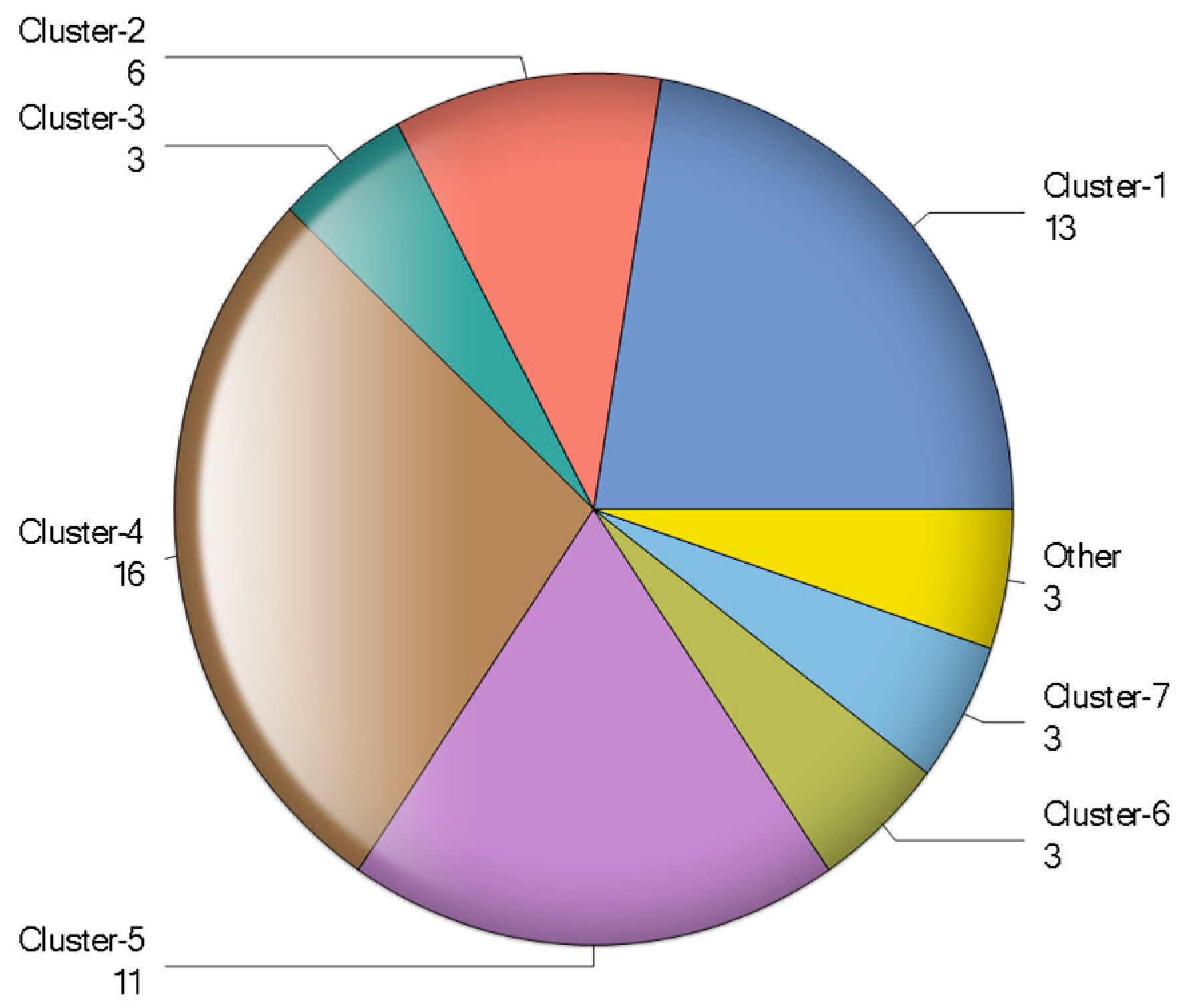
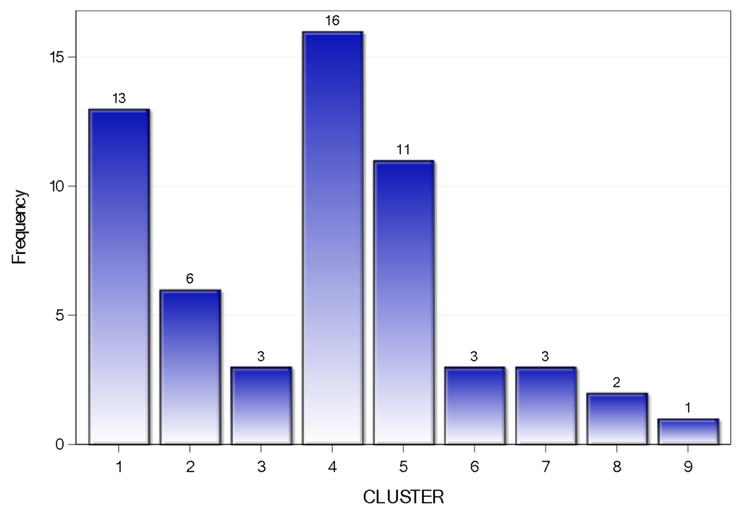
| Cluster | Frequency | Percent | Cumulative Frequency | Cumulative Percent |
|---|---|---|---|---|
| Cluster-1 | 13 | 22.41 | 12 | 68.97 |
| Cluster-2 | 6 | 10.34 | 19 | 84.48 |
| Cluster-3 | 3 | 5.17 | 22 | 74.14 |
| Cluster-4 | 16 | 27.59 | 38 | 46.55 |
| Cluster-5 | 11 | 18.97 | 49 | 18.97 |
| Cluster-6 | 3 | 5.17 | 52 | 89.66 |
| Cluster-7 | 3 | 5.17 | 55 | 98.28 |
| Cluster-8 | 2 | 3.45 | 57 | 93.10 |
| Cluster-9 | 1 | 1.72 | 58 | 100.00 |
| Clusters | Statistics | Frequency | Assets Growth | GDP Growth | NPL/Loans | Total Assets |
|---|---|---|---|---|---|---|
| Sample | Mean | 10.01 | 5.16 | 4.24 | 187,224.90 | |
| Median | 10.38 | 5.23 | 3.15 | 32,380.45 | ||
| CV | 107.48 | 61.78 | 87.33 | 259.73 | ||
| Skewness | 0.07 | −0.21 | 1.90 | 4.24 | ||
| Kurtosis | 0.99 | 1.31 | 4.04 | 19.20 | ||
| Cluster-1 | Mean | 13 | 11.17 | 5.82 | 4.58 | 45,945.75 |
| Median | 11.38 | 5.64 | 4.43 | 8027.08 | ||
| CV | 13.91 | 9.84 | 25.34 | 190.72 | ||
| Skewness | −0.78 | 0.89 | 1.19 | 2.86 | ||
| Kurtosis | −0.17 | 2.28 | 0.96 | 8.67 | ||
| Cluster-2 | Mean | 6 | 15.71 | 6.83 | 1.78 | 21,990.68 |
| Median | 16.01 | 7.14 | 1.64 | 8783.72 | ||
| CV | 12.10 | 8.06 | 38.05 | 121.11 | ||
| Skewness | 0.03 | −0.91 | 1.51 | 1.00 | ||
| Kurtosis | −0.37 | −1.88 | 2.52 | −1.29 | ||
| Cluster-3 | Mean | 3 | 17.92 | 9.26 | 1.07 | 543,580.65 |
| Median | 18.40 | 9.26 | 0.99 | 481,710.87 | ||
| CV | 9.02 | 0.00 | 22.67 | 27.68 | ||
| Skewness | −1.23 | 1.31 | 1.54 | |||
| Cluster-4 | Mean | 16 | 6.92 | 4.43 | 2.40 | 105,430.02 |
| Median | 7.32 | 4.85 | 2.77 | 82,865.12 | ||
| CV | 30.69 | 19.15 | 44.75 | 78.14 | ||
| Skewness | −0.24 | −0.21 | −0.25 | 0.75 | ||
| Kurtosis | −0.81 | −1.50 | −1.07 | −0.50 | ||
| Cluster-5 | Mean | 11 | 9.66 | 3.30 | 5.69 | 58,061.85 |
| Median | 9.97 | 3.45 | 5.51 | 8502.77 | ||
| CV | 20.99 | 8.23 | 29.26 | 213.44 | ||
| Skewness | −0.71 | −1.08 | 0.86 | 3.15 | ||
| Kurtosis | 1.05 | 1.26 | 0.17 | 10.16 | ||
| Cluster-6 | Mean | 3 | 13.59 | 9.26 | 1.74 | 2,028,139.68 |
| Median | 13.59 | 9.26 | 1.57 | 1,922,427.58 | ||
| CV | 4.41 | 0.00 | 23.52 | 15.89 | ||
| Skewness | 0.02 | 1.56 | 1.32 | |||
| Cluster-7 | Mean | 3 | 3.68 | 2.48 | 13.79 | 20,778.74 |
| Median | 4.28 | 3.45 | 13.95 | 13,033.19 | ||
| CV | 79.03 | 67.51 | 5.47 | 106.01 | ||
| Skewness | −0.89 | −1.73 | −0.94 | 1.39 | ||
| Cluster-8 | Mean | 2 | 0.20 | 3.30 | 7.82 | 13,180.11 |
| Median | 0.20 | 3.30 | 7.82 | 13,180.11 | ||
| CV | 391.08 | 6.34 | 22.38 | 83.45 | ||
| Cluster-9 | Mean | 1 | 18.14 | 6.10 | 9.44 | 387.31 |
| Median | 18.14 | 6.10 | 9.44 | 387.31 |
| Clusters | Country | Name of Banks in Each Cluster | ||||
|---|---|---|---|---|---|---|
| 1 | Sri Lanka | Ceylon | Hatton | Sampath | DFCC | |
| Philippines | China Bank | PNB | RCBC | BDO | ||
| Indonesia | BRI | Mandiri | ||||
| India | ICICI | |||||
| Bangladesh | Prime | |||||
| Malaysia | CIMB | |||||
| 2 | India | AXIS | Indusind | HDFC | Southindian | |
| Sri Lanka | NDB | |||||
| Bangladesh | Dutch Bungla | |||||
| 3 | China | China Merchant | Communication | SPD | ||
| 4 | Turkey | AKBank | BCA | Garanti | ISbank | Yapi |
| Malaysia | AMMB | Hong-Leong | Maybank | |||
| Thailand | Bankok | |||||
| Indonesia | Danamon | |||||
| Singapore | DBS | OCBC | UOB | |||
| Nepal | Himalayan | |||||
| 5 | Turkey | ABank | Seker | |||
| Pakistan | ABL | MCB | UBL | |||
| Chile | De-Chile | |||||
| Brazil | Do-Brazil | |||||
| Thailand | Kiatnakin | KTB | Siam | Thanachart | ||
| 6 | China | Bankofchina | CCB | ICBC | ||
| 7 | Pakistan | Askari | NBP | |||
| Hungary | OTP | |||||
| 8 | Pakistan | BankAlfalah | ||||
| Thailand | TMB | |||||
| 9 | Sri Lanka | PABC | ||||
| Variables | Signs | Estimates | t-Value | SE |
|---|---|---|---|---|
| ROAE | + | 0.3775 *** | 23.97 | 0.0157 |
| CEO SAB | + | 0.0829 *** | 9.07 | 0.0091 |
| MD&A SAB | + | 0.0806 *** | 4.01 | 0.0201 |
| Fit Statistics | ||||
| RMSE | 0.8897 | |||
| MSE | 0.7915 | |||
| SSE | 317.39 | |||
| Diagnostic Tests | ||||
| AR(m) Test Lag 1 (Statistic) | 2.47 ** | |||
| p > |Statistic| | (0.0136) | |||
| AR(m) Test Lag 2 (Statistic) | 0.40 | |||
| p > |Statistic| | (0.6918) | |||
| Sargan Test (Statistic) | 51.01 | |||
| p > ChiSq | (0.4695) |
| Variables | Sign | Estimates | t-Value | SE |
|---|---|---|---|---|
| ROAE | + | 0.2980 *** | 12.01 | 0.0248 |
| CEO SAB | + | 0.0354 | 1.55 | 0.0229 |
| MD&A SAB | + | 0.1474 *** | 3.00 | 0.0492 |
| Total Assets (log) | - | 0.5283 *** | 4.51 | 0.1173 |
| Assets Growth (%) | + | 0.1104 *** | 3.99 | 0.0277 |
| NPL/Gross Loans (%) | - | 0.2398 *** | 2.85 | 0.0840 |
| Tier1Capital (%) | - | 0.4379 *** | 6.21 | 0.0705 |
| Loans/Assets (%) | - | 0.3260 *** | 5.16 | 0.0631 |
| Fit Statistics | ||||
| RMSE | 0.8437 | |||
| MSE | 0.7119 | |||
| SSE | 281.91 | |||
| Diagnostic Test | ||||
| AR(m) Test Lag 1 (Statistic) | −2.50 *** | |||
| p > |Statistic| | (0.0125) | |||
| AR(m) Test Lag 2 (Statistic) | 0.12 | |||
| p > |Statistic| | (0.9051) | |||
| Sargan Test (Statistic) | 48.65 | |||
| p > ChiSq | (0.5275) |
| Variables | Sign | Estimates | t-Value | SE |
|---|---|---|---|---|
| ROAE | + | 0.2284 *** | 6.58 | 0.0347 |
| CEO SAB | + | 0.0580 ** | 2.21 | 0.0262 |
| MD&A SAB | + | 0.1360 *** | 3.18 | 0.0428 |
| Assets (log) | − | 0.3877 ** | 2.37 | 0.1634 |
| Assets Growth (%) | + | 0.1466 *** | 4.41 | 0.0332 |
| NPL/Gross Loans (%) | − | 0.2259 *** | 2.83 | 0.0798 |
| Tier1Capital (%) | − | 0.5513 *** | 7.85 | 0.0703 |
| Loans/Assets (%) | − | 0.3782 *** | 4.02 | 0.0941 |
| Interest Rate Spread (%) | + | 0.1737 | 1.49 | 0.1164 |
| GDP Growth (%) | − | 0.0031 | 0.08 | 0.0383 |
| Exchange Rate (%) | − | 0.1829 | 0.88 | 0.2081 |
| Fit Statistics | ||||
| RMSE | 0.8390 | |||
| MSE | 0.7040 | |||
| SSE | 276.66 | |||
| Diagnostic Test | ||||
| AR(m) Test Lag 1 (Statistic) | −2.41 *** | |||
| p > |Statistic| | 0.0159 | |||
| AR(m) Test Lag 2 (Statistic) | −0.07 | |||
| p > |Statistic| | 0.9422 | |||
| Sargan Test (Statistic) | 51.01 | |||
| p > ChiSq | 0.3189 |
© 2019 by the author. Licensee MDPI, Basel, Switzerland. This article is an open access article distributed under the terms and conditions of the Creative Commons Attribution (CC BY) license (http://creativecommons.org/licenses/by/4.0/).
Share and Cite
Iqbal, J. Managerial Self-Attribution Bias and Banks’ Future Performance: Evidence from Emerging Economies. J. Risk Financial Manag. 2019, 12, 73. https://doi.org/10.3390/jrfm12020073
Iqbal J. Managerial Self-Attribution Bias and Banks’ Future Performance: Evidence from Emerging Economies. Journal of Risk and Financial Management. 2019; 12(2):73. https://doi.org/10.3390/jrfm12020073
Chicago/Turabian StyleIqbal, Javid. 2019. "Managerial Self-Attribution Bias and Banks’ Future Performance: Evidence from Emerging Economies" Journal of Risk and Financial Management 12, no. 2: 73. https://doi.org/10.3390/jrfm12020073
APA StyleIqbal, J. (2019). Managerial Self-Attribution Bias and Banks’ Future Performance: Evidence from Emerging Economies. Journal of Risk and Financial Management, 12(2), 73. https://doi.org/10.3390/jrfm12020073