Efficient Numerical Pricing of American Call Options Using Symmetry Arguments


Abstract
1. Introduction
2. Motivation
2.1. Regular Call Option Prices
2.2. Call Options Priced by Symmetry
3. Implementation
3.1. Simulation and Regression Methods
3.2. Implementation of the LSMC Method
4. Results
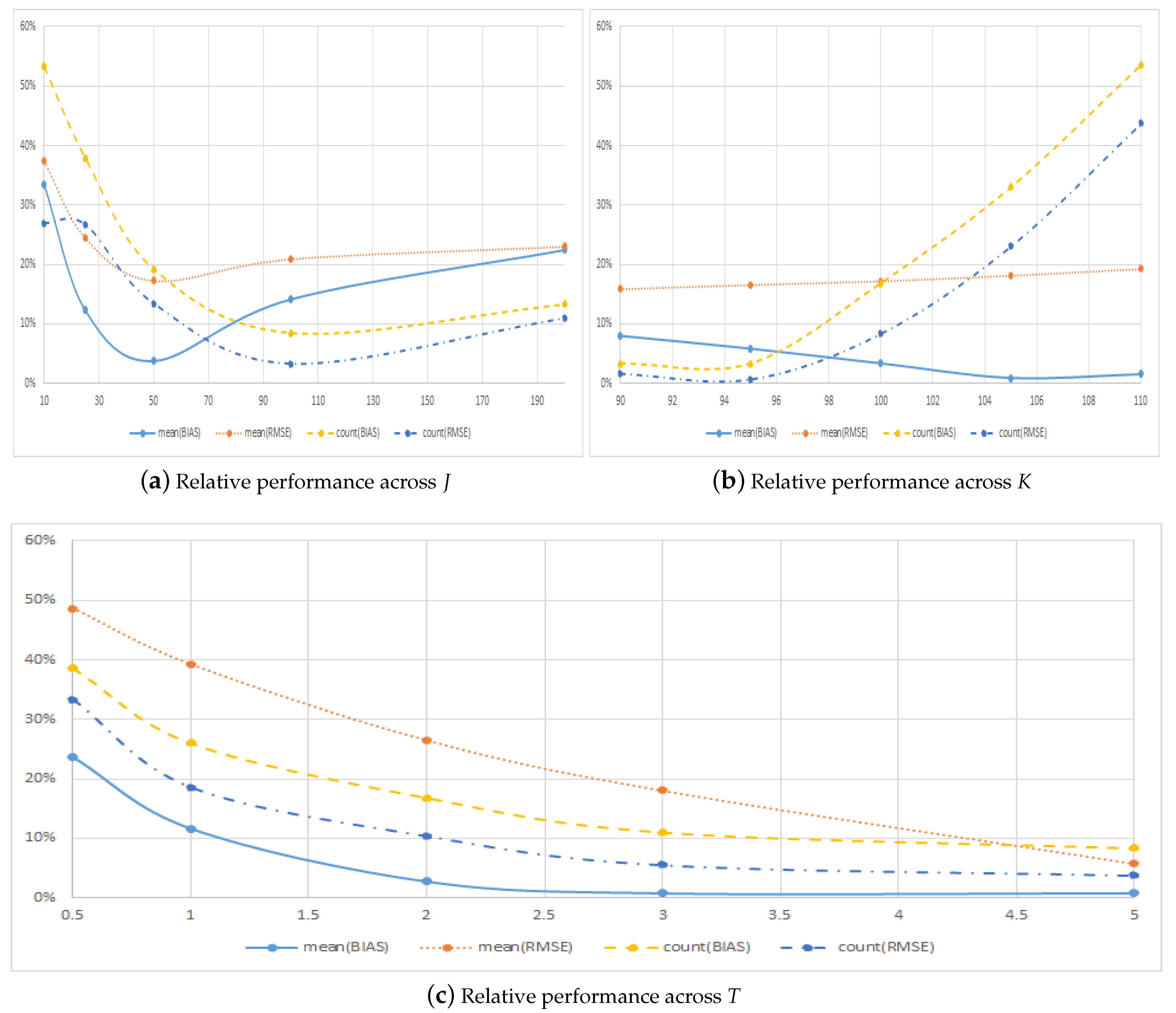
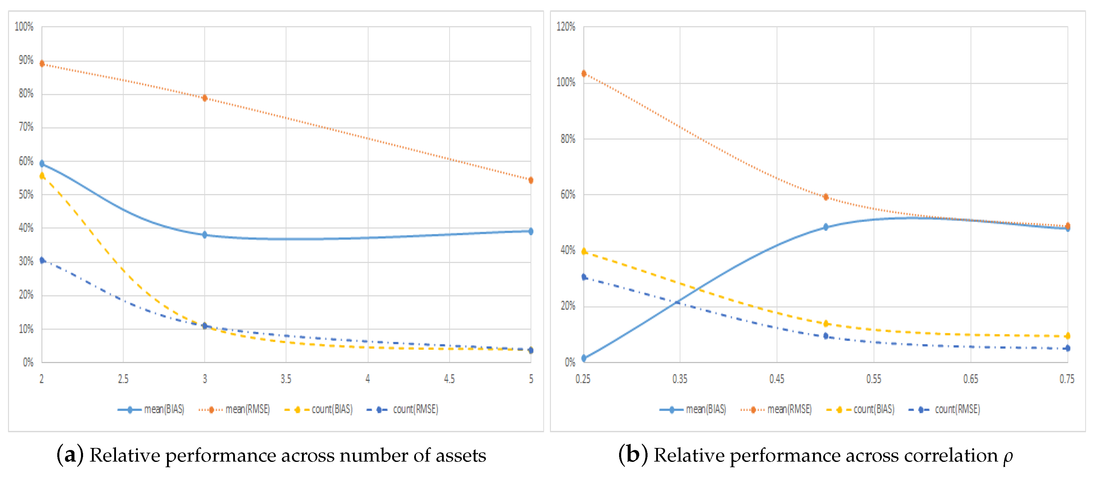
4.1. Performance across Option Characteristics
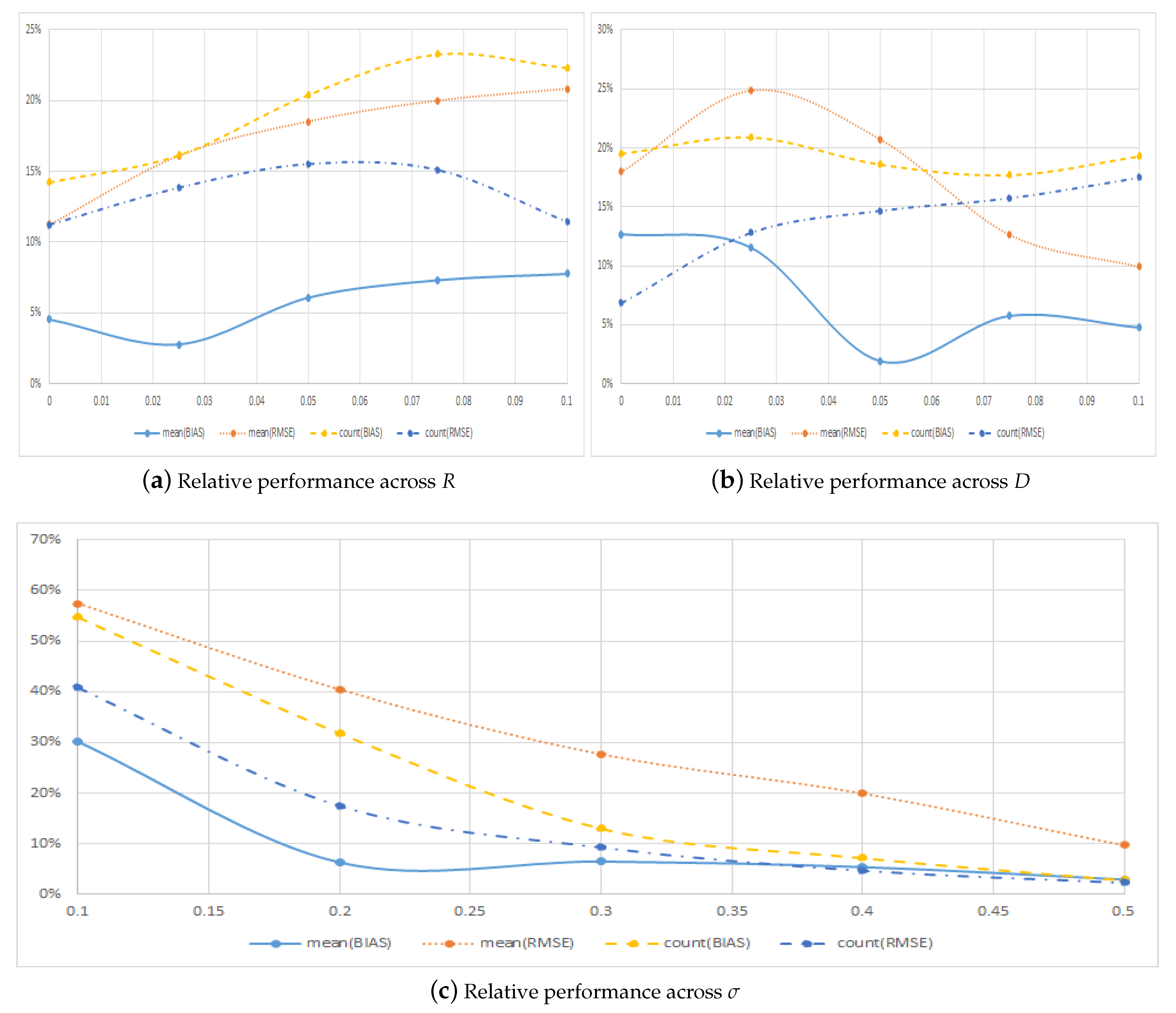
4.2. Performance across Model Parameters
5. Robustness
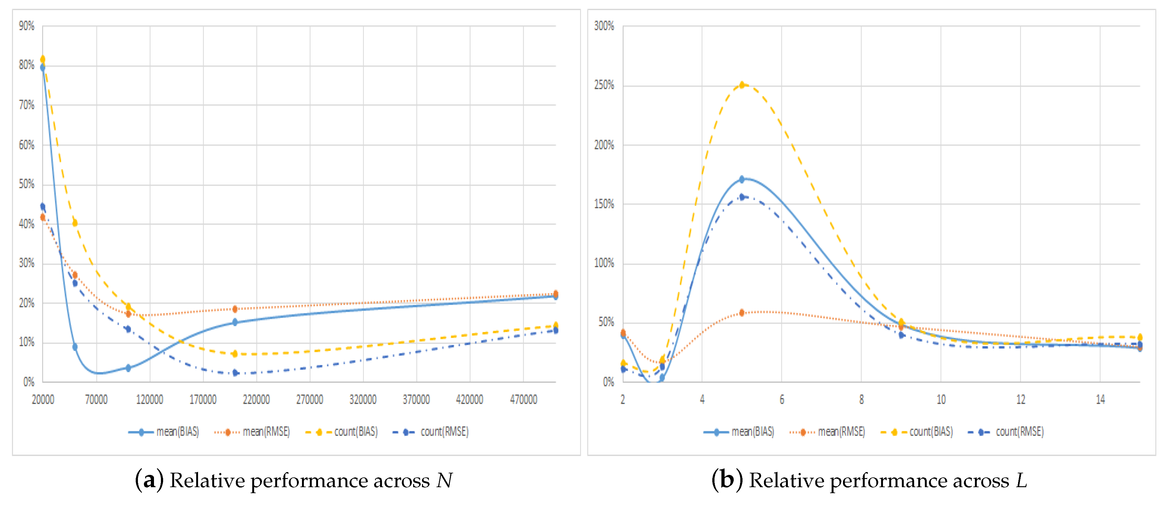
5.1. Alternative Choices for the Number of Paths and Regressors
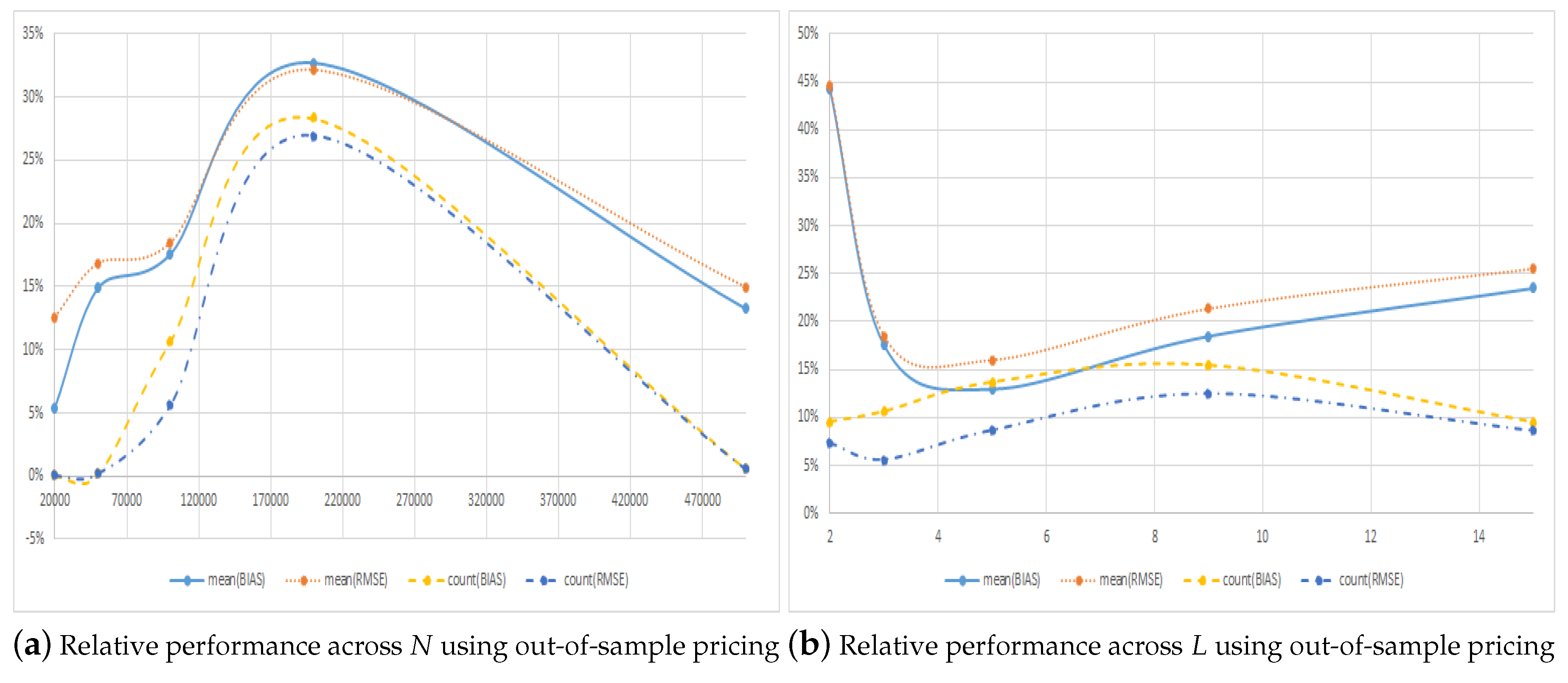
5.2. Extensions to Other Option Pricing Models
6. Discussion
6.1. Efficiency as an Alternative Metric
6.2. Picking the Best Configuration
7. Conclusions
Funding
Acknowledgments
Conflicts of Interest
References
- Battauz, Anna, Marzia De Donno, and Alessandro Sbuelz. 2014. The Put-Call Symmetry for American Options in the Heston Stochastic Volatility Model. Mathematical Finance Letters 7: 1–8. [Google Scholar]
- Boyle, Phelim P., and Yiu Kuen Tse. 1990. An Algorithm for Computing Values of Options on the Maximum or Minimum of Several Assets. Journal of Financial and Quantitative Analysis 25: 215–27. [Google Scholar] [CrossRef]
- Chow, Yuan-Shih, Herbert Robbins, and David Siegmund. 1971. Great Expectations: The Theory of Optimal Stopping. New York: Houghton Mifflin. [Google Scholar]
- Cox, John C., Jonathan E. Ingersoll, and Stephen A. Ross. 1985. A Theory of the Term Structure of Interest Rates. Econometrica 53: 385–408. [Google Scholar] [CrossRef]
- Cox, John C., Stephen A. Ross, and Mark Rubinstein. 1979. Option pricing: A simplified approach. Journal of Financial Economics 7: 229–63. [Google Scholar] [CrossRef]
- Detemple, Jerome. 2001. American Options: Symmetry Properties. In Handbooks in Mathematical Finance: Topics in Option Pricing, Interest Rates and Risk Management. Edited by Elyes Jouini, Jaksa Cvitanic and Marek Musiela. Cambridge: Cambridge University Press, pp. 67–104. [Google Scholar]
- Duffie, Darrell. 1996. Dynamic Asset Pricing Theory. Princeton: Princeton University Press. [Google Scholar]
- Grabbe, J. Orlin. 1983. The Pricing of Call and Put Options of Foreign Exchange. Journal of International Money and Finance 2: 239–53. [Google Scholar] [CrossRef]
- Heston, Steven L. 1993. A Closed-Form Solution for Options with Stochastic Volatility with Applications to Bond and Currency Options. Review of Financial Studies 6: 327–43. [Google Scholar] [CrossRef]
- Hull, John, and Alan White. 1987. The Pricing of Options on Assets with Stochastic Volatilities. Journal of Finance 42: 281–300. [Google Scholar] [CrossRef]
- Karatzas, Ioannis. 1988. On the Pricing of American Options. Applied Mathematics and Optimization 17: 37–60. [Google Scholar] [CrossRef]
- Longstaff, Francis A., and Eduardo S. Schwartz. 2001. Valuing American Options by Simulation: A Simple Least-Squares Approach. Review of Financial Studies 14: 113–47. [Google Scholar] [CrossRef]
- McDonald, Robert C., and Mark Schroder. 1998. A Parity Result for American Options. Journal of Computational Finance 1: 5–13. [Google Scholar] [CrossRef]
- Royden, Halsey. 1988. Real Analysis. Upper Saddle River: Prentice Hall, Inc. [Google Scholar]
- Schroder, Mark. 1999. Changes of Numeraire for Pricing Futures, Forwards, and Options. Review of Financial Studies 12: 1143–63. [Google Scholar] [CrossRef]
- Scott, Louis O. 1987. Option Pricing When the Variance Changes Radomly: Theory, Estimation, and an Application. Journal of Financial and Quantitative Analysis 22: 419–38. [Google Scholar] [CrossRef]
- Stentoft, Lars. 2004a. Assessing the Least Squares Monte-Carlo Approach to American Option Valuation. Review of Derivatives Research 7: 129–68. [Google Scholar] [CrossRef]
- Stentoft, Lars. 2004b. Convergence of the Least Squares Monte Carlo Approach to American Option Valuation. Management Science 50: 1193–203. [Google Scholar] [CrossRef]
- Wiggins, James B. 1987. Option Values Under Stochastic Volatility: Theory and Empirical Estimates. Journal of Financial Economics 19: 351–72. [Google Scholar] [CrossRef]
| 1. | For example, PCS also holds in the stochastic volatility model of Heston (1993) when the parameters of the volatility process and the correlation are changed appropriately. See, e.g., Battauz et al. (2014) for the exact specification, Grabbe (1983) for an intuitive explanation of how to derive the relationship using options on foreign exchange and Detemple (2001) for extensions to derivatives on multiple assets. |
| 2. | The main parts of the paper present results for the simple Black–Scholes–Merton setup. The reason for this is obvious: we want to have fast and precise benchmark results available. Without these, it makes no sense to talk about one method being more efficient than another. Section 5, though, shows that these conclusions extend to other asset dynamics, like the stochastic volatility model of Heston (1993), and to options with other payoff functions, like options written on multivariate underlying assets. |
| 3. | Although the path-wise payoffs obtained with the LSMC method for a given Monte Carlo simulation are dependent and could be very far from normally distributed, the price estimates we report in the table are averages of independent simulations and should therefore be normally distributed by a central limit theorem. The actual values for the skewness and excess kurtosis are not shown in the table, but are available upon request. |
| 4. | This is justified when approximating elements of the space of square-integrable functions relative to some measure. Since is a Hilbert space, it has a countable orthonormal basis (see, e.g., Royden 1988). |
| 5. | For now, we maintain the assumption that dynamics are governed by simple geometric Brownian motion. However, our results generalize to other models for which PCS holds, as we demonstrate in Section 5. |
| 6. | We deal with the difference in, for example, the payoff when exercising the option by using negative values for the strike price and the stock prices for put options since . |
| 7. | Unreported results, available upon request, show that this generalizes to the much larger sample of options we consider in Section 4. |
| 8. | This follows from the Weierstrass approximation theorem, which states that every continuous function defined on a closed interval can be uniformly approximated as closely as desired by a polynomial function. |
| 9. | Using the fraction of times a given method has the highest error metric ensures, as is the case with the bias and RMSE error metrics, that lower numbers are better. |
| 10. | Note, though, that, e.g., the bias of both the regular and symmetric method increases in absolute terms when increasing the number of exercise points. This is likely related to the fact that dependence is introduced between the paths in the LSMC method because of the cross-sectional regression, and this dependence “accumulates” as we go backwards in time in the algorithm and becomes more and more important as the number of early exercise possibilities increases. |
| 11. | Again, for all other values of the number of simulated paths with this number of regressors and when using other numbers of regressors with this number of simulated paths, the symmetric estimates are less biased. |
| 12. | The working version of this paper contains the full details on how to derive these dynamics. |
| 13. | These numbers are the “inverse” of the counting metrics used in previous tables. |
| 14. | The mode of the number of regressors, L, for the regular method is seven, on the other hand. |


| BM | Regular Call | Rel. | Symmetric Call | |||||||||
|---|---|---|---|---|---|---|---|---|---|---|---|---|
| Price | Price | Bias | StDev | RMSE | RMSE | Price | Bias | StDev | RMSE | |||
| 36 | 1 | 0.20 | 5.2247 | 5.2236 | −0.0011 | (0.0074) | 0.0013 | 1.44 | 5.2240 | −0.0007 | (0.0059) | 0.0009 |
| 38 | 1 | 0.20 | 4.0292 | 4.0278 | −0.0014 | (0.0088) | 0.0016 | 1.09 | 4.0278 | −0.0014 | (0.0050) | 0.0015 |
| 40 | 1 | 0.20 | 3.0420 | 3.0417 | −0.0003 | (0.0106) | 0.0011 | 1.21 | 3.0414 | −0.0006 | (0.0071) | 0.0009 |
| 42 | 1 | 0.20 | 2.2502 | 2.2508 | 0.0006 | (0.0099) | 0.0012 | 1.52 | 2.2503 | 0.0001 | (0.0075) | 0.0008 |
| 44 | 1 | 0.20 | 1.6324 | 1.6331 | 0.0007 | (0.0100) | 0.0012 | 1.52 | 1.6328 | 0.0004 | (0.0070) | 0.0008 |
| 36 | 1 | 0.40 | 7.8808 | 7.8777 | −0.0031 | (0.0225) | 0.0038 | 1.92 | 7.8790 | −0.0018 | (0.0083) | 0.0020 |
| 38 | 1 | 0.40 | 6.9153 | 6.9147 | −0.0006 | (0.0244) | 0.0025 | 1.30 | 6.9135 | −0.0018 | (0.0076) | 0.0019 |
| 40 | 1 | 0.40 | 6.0543 | 6.0542 | −0.0001 | (0.0259) | 0.0026 | 2.24 | 6.0537 | −0.0006 | (0.0101) | 0.0012 |
| 42 | 1 | 0.40 | 5.2900 | 5.2905 | 0.0005 | (0.0241) | 0.0025 | 1.92 | 5.2901 | 0.0001 | (0.0128) | 0.0013 |
| 44 | 1 | 0.40 | 4.6141 | 4.6161 | 0.0021 | (0.0235) | 0.0031 | 2.34 | 4.6145 | 0.0004 | (0.0127) | 0.0013 |
| 36 | 2 | 0.20 | 6.0796 | 6.0771 | −0.0025 | (0.0103) | 0.0027 | 2.40 | 6.0787 | −0.0009 | (0.0070) | 0.0011 |
| 38 | 2 | 0.20 | 5.0249 | 5.0232 | 0.0016 | (0.0119) | 0.0020 | 2.37 | 5.0244 | 0.0005 | (0.0071) | 0.0009 |
| 40 | 2 | 0.20 | 4.1221 | 4.1210 | 0.0010 | (0.0135) | 0.0017 | 2.25 | 4.1218 | 0.0002 | (0.0072) | 0.0008 |
| 42 | 2 | 0.20 | 3.3578 | 3.3577 | 0.0001 | (0.0132) | 0.0013 | 1.30 | 3.3572 | 0.0006 | (0.0079) | 0.0010 |
| 44 | 2 | 0.20 | 2.7174 | 2.7182 | 0.0008 | (0.0126) | 0.0015 | 1.67 | 2.7173 | 0.0001 | (0.0090) | 0.0009 |
| 36 | 2 | 0.40 | 9.7706 | 9.6202 | 0.1504 | (0.1055) | 0.1508 | 113.89 | 9.7700 | 0.0006 | (0.0120) | 0.0013 |
| 38 | 2 | 0.40 | 8.9315 | 8.8415 | 0.0900 | (0.0844) | 0.0904 | 64.28 | 8.9306 | 0.0009 | (0.0112) | 0.0014 |
| 40 | 2 | 0.40 | 8.1661 | 8.1128 | 0.0533 | (0.0634) | 0.0537 | 38.56 | 8.1652 | 0.0009 | (0.0106) | 0.0014 |
| 42 | 2 | 0.40 | 7.4684 | 7.4352 | 0.0332 | (0.0496) | 0.0336 | 30.01 | 7.4682 | 0.0002 | (0.0111) | 0.0011 |
| 44 | 2 | 0.40 | 6.8323 | 6.8132 | 0.0191 | (0.0411) | 0.0195 | 15.19 | 6.8317 | 0.0006 | (0.0116) | 0.0013 |
| Panel A: Across Early Exercise Points J | ||||||||
|---|---|---|---|---|---|---|---|---|
| Absolute Metrics | Counting Metrics | |||||||
| Regular Call | Symmetric Call | Regular Call | Symmetric Call | |||||
| J | Bias | RMSE | Bias | RMSE | Bias | RMSE | Bias | RMSE |
| 10 | −0.0066 | 0.0169 | 0.0022 | 0.0063 | 0.6525 | 0.7878 | 0.3475 | 0.2122 |
| 25 | −0.0310 | 0.0351 | 0.0038 | 0.0086 | 0.7251 | 0.7894 | 0.2749 | 0.2106 |
| 50 | −0.0574 | 0.0602 | −0.0022 | 0.0104 | 0.8390 | 0.8819 | 0.1610 | 0.1181 |
| 100 | −0.0639 | 0.0660 | −0.0090 | 0.0138 | 0.9222 | 0.9683 | 0.0778 | 0.0317 |
| 200 | −0.0922 | 0.0963 | −0.0207 | 0.0222 | 0.8829 | 0.9014 | 0.1171 | 0.0986 |
| Panel B: Across Strike Prices | ||||||||
| Absolute Metrics | Counting Metrics | |||||||
| Regular Call | Symmetric Call | Regular Call | Symmetric Call | |||||
| K | Bias | RMSE | Bias | RMSE | Bias | RMSE | Bias | RMSE |
| 90 | −0.0682 | 0.0707 | −0.0055 | 0.0112 | 0.9680 | 0.9840 | 0.0320 | 0.0160 |
| 95 | −0.0631 | 0.0657 | −0.0037 | 0.0109 | 0.9680 | 0.9936 | 0.0320 | 0.0064 |
| 100 | −0.0574 | 0.0602 | −0.0019 | 0.0104 | 0.8560 | 0.9232 | 0.1440 | 0.0768 |
| 105 | −0.0521 | 0.0550 | −0.0005 | 0.0100 | 0.7520 | 0.8128 | 0.2480 | 0.1872 |
| 110 | −0.0464 | 0.0495 | 0.0007 | 0.0096 | 0.6512 | 0.6960 | 0.3488 | 0.3040 |
| Panel C: Across Maturity | ||||||||
| Absolute Metrics | Counting Metrics | |||||||
| Regular Call | Symmetric Call | Regular Call | Symmetric Call | |||||
| T | Bias | RMSE | Bias | RMSE | Bias | RMSE | Bias | RMSE |
| 0.5 | −0.0211 | 0.0220 | −0.0050 | 0.0107 | 0.7216 | 0.7504 | 0.2784 | 0.2496 |
| 1 | −0.0279 | 0.0293 | −0.0032 | 0.0115 | 0.7936 | 0.8432 | 0.2064 | 0.1568 |
| 2 | −0.0392 | 0.0414 | −0.0011 | 0.0110 | 0.8560 | 0.9056 | 0.1440 | 0.0944 |
| 3 | −0.0525 | 0.0553 | −0.0004 | 0.0100 | 0.9008 | 0.9472 | 0.0992 | 0.0528 |
| 5 | −0.1462 | 0.1531 | −0.0011 | 0.0089 | 0.9232 | 0.9632 | 0.0768 | 0.0368 |
| Panel A: Across Interest Rates r | ||||||||
|---|---|---|---|---|---|---|---|---|
| Absolute Metrics | Counting Metrics | |||||||
| Regular Call | Symmetric Call | Regular Call | Symmetric Call | |||||
| bias | RMSE | Bias | RMSE | Bias | RMSE | Bias | RMSE | |
| 0% | −0.0560 | 0.0574 | 0.0025 | 0.0065 | 0.8752 | 0.8992 | 0.1248 | 0.1008 |
| 2.5% | −0.0656 | 0.0673 | −0.0018 | 0.0108 | 0.8608 | 0.8784 | 0.1392 | 0.1216 |
| 5.0% | −0.0618 | 0.0643 | −0.0038 | 0.0119 | 0.8304 | 0.8656 | 0.1696 | 0.1344 |
| 7.5% | −0.0553 | 0.0590 | −0.0040 | 0.0118 | 0.8112 | 0.8688 | 0.1888 | 0.1312 |
| 10% | −0.0484 | 0.0530 | −0.0038 | 0.0110 | 0.8176 | 0.8976 | 0.1824 | 0.1024 |
| Panel B: Across Dividend Yields | ||||||||
| Absolute Metrics | Counting Metrics | |||||||
| Regular Call | Symmetric Call | Regular Call | Symmetric Call | |||||
| Bias | RMSE | Bias | RMSE | Bias | RMSE | Bias | RMSE | |
| 0% | −0.0730 | 0.0789 | −0.0093 | 0.0142 | 0.8368 | 0.9360 | 0.1632 | 0.0640 |
| 2.5% | −0.0555 | 0.0591 | −0.0064 | 0.0147 | 0.8272 | 0.8864 | 0.1728 | 0.1136 |
| 5.0% | −0.0487 | 0.0509 | −0.0009 | 0.0106 | 0.8432 | 0.8720 | 0.1568 | 0.1280 |
| 7.5% | −0.0527 | 0.0542 | 0.0030 | 0.0069 | 0.8496 | 0.8640 | 0.1504 | 0.1360 |
| 10% | −0.0571 | 0.0580 | 0.0027 | 0.0058 | 0.8384 | 0.8512 | 0.1616 | 0.1488 |
| Panel C: Across Volatility Levels | ||||||||
| Absolute Metrics | Counting Metrics | |||||||
| Regular Call | Symmetric Call | Regular Call | Symmetric Call | |||||
| Bias | RMSE | Bias | RMSE | Bias | RMSE | Bias | RMSE | |
| 10% | −0.0034 | 0.0046 | 0.0010 | 0.0026 | 0.6464 | 0.7104 | 0.3536 | 0.2896 |
| 20% | −0.0162 | 0.0186 | −0.0010 | 0.0075 | 0.7584 | 0.8512 | 0.2416 | 0.1488 |
| 30% | −0.0382 | 0.0411 | −0.0025 | 0.0114 | 0.8848 | 0.9152 | 0.1152 | 0.0848 |
| 40% | −0.0694 | 0.0716 | −0.0037 | 0.0143 | 0.9328 | 0.9552 | 0.0672 | 0.0448 |
| 50% | −0.1598 | 0.1652 | −0.0047 | 0.0161 | 0.9728 | 0.9776 | 0.0272 | 0.0224 |
| Panel A: Across Number of Simulated Paths N | ||||||||
|---|---|---|---|---|---|---|---|---|
| Absolute Metrics | Counting Metrics | |||||||
| Regular Call | Symmetric Call | Regular Call | Symmetric Call | |||||
| Bias | RMSE | Bias | RMSE | Bias | RMSE | Bias | RMSE | |
| 20,000 | −0.0112 | 0.0426 | 0.0089 | 0.0178 | 0.5498 | 0.6915 | 0.4502 | 0.3085 |
| 50,000 | −0.0428 | 0.0480 | 0.0038 | 0.0131 | 0.7130 | 0.8000 | 0.2870 | 0.2000 |
| 100,000 | −0.0574 | 0.0602 | −0.0022 | 0.0104 | 0.8390 | 0.8819 | 0.1610 | 0.1181 |
| 200,000 | −0.0526 | 0.0540 | −0.0080 | 0.0100 | 0.9322 | 0.9766 | 0.0678 | 0.0234 |
| 500,000 | −0.0549 | 0.0556 | −0.0120 | 0.0124 | 0.8749 | 0.8835 | 0.1251 | 0.1165 |
| Panel B: Across Number of Regressors | ||||||||
| Absolute Metrics | Counting Metrics | |||||||
| Regular Call | Symmetric Call | Regular Call | Symmetric Call | |||||
| Bias | RMSE | Bias | RMSE | Bias | RMSE | Bias | RMSE | |
| 2 | −0.0819 | 0.0832 | −0.0330 | 0.0351 | 0.8608 | 0.8986 | 0.1392 | 0.1014 |
| 3 | −0.0574 | 0.0602 | −0.0022 | 0.0104 | 0.8390 | 0.8819 | 0.1610 | 0.1181 |
| 5 | −0.0061 | 0.0201 | 0.0104 | 0.0117 | 0.2848 | 0.3901 | 0.7152 | 0.6099 |
| 9 | 0.0296 | 0.0328 | 0.0144 | 0.0154 | 0.6611 | 0.7123 | 0.3389 | 0.2877 |
| 15 | 0.0614 | 0.0625 | 0.0178 | 0.0187 | 0.7261 | 0.7555 | 0.2739 | 0.2445 |
| Panel A: Across Number of Simulated Paths N | ||||||||
|---|---|---|---|---|---|---|---|---|
| Absolute Metrics | Counting Metrics | |||||||
| Regular Call | Symmetric Call | Regular Call | Symmetric Call | |||||
| Bias | RMSE | Bias | RMSE | Bias | RMSE | Bias | RMSE | |
| 20,000 | −0.1286 | 0.1303 | −0.0070 | 0.0163 | 0.9997 | 0.9997 | 0.0003 | 0.0003 |
| 50,000 | −0.0974 | 0.0986 | −0.0145 | 0.0166 | 0.9984 | 0.9978 | 0.0016 | 0.0022 |
| 100,000 | −0.0837 | 0.0851 | −0.0147 | 0.0157 | 0.9040 | 0.9472 | 0.0960 | 0.0528 |
| 200,000 | −0.0565 | 0.0590 | −0.0185 | 0.0190 | 0.7792 | 0.7878 | 0.2208 | 0.2122 |
| 500,000 | −0.0706 | 0.0708 | −0.0094 | 0.0106 | 0.9939 | 0.9942 | 0.0061 | 0.0058 |
| Panel B: Across Number of Regressors | ||||||||
| Absolute Metrics | Counting Metrics | |||||||
| Regular Call | Symmetric Call | Regular Call | Symmetric Call | |||||
| Bias | RMSE | Bias | RMSE | Bias | RMSE | Bias | RMSE | |
| 2 | −0.0974 | 0.0983 | −0.0431 | 0.0438 | 0.9130 | 0.9322 | 0.0870 | 0.0678 |
| 3 | −0.0837 | 0.0851 | −0.0147 | 0.0157 | 0.9040 | 0.9472 | 0.0960 | 0.0528 |
| 5 | −0.0488 | 0.0498 | −0.0063 | 0.0079 | 0.8797 | 0.9203 | 0.1203 | 0.0797 |
| 9 | −0.0418 | 0.0427 | −0.0077 | 0.0091 | 0.8662 | 0.8890 | 0.1338 | 0.1110 |
| 15 | −0.0450 | 0.0458 | −0.0106 | 0.0117 | 0.9133 | 0.9210 | 0.0867 | 0.0790 |
| Panel A: Across Number of Assets M | ||||||||
|---|---|---|---|---|---|---|---|---|
| Absolute Metrics | Counting Metrics | |||||||
| Regular Call | Symmetric Call | Regular Call | Symmetric Call | |||||
| Bias | RMSE | Bias | RMSE | Bias | RMSE | Bias | RMSE | |
| 2 | 0.0021 | 0.0054 | 0.0012 | 0.0048 | 0.6420 | 0.7654 | 0.3580 | 0.2346 |
| 3 | 0.0099 | 0.0123 | 0.0038 | 0.0097 | 0.9012 | 0.9012 | 0.0988 | 0.0988 |
| 5 | 0.0319 | 0.0329 | 0.0125 | 0.0180 | 0.9630 | 0.9630 | 0.0370 | 0.0370 |
| Panel B: Across Correlation | ||||||||
| Absolute Metrics | Counting Metrics | |||||||
| Regular Call | Symmetric Call | Regular Call | Symmetric Call | |||||
| Bias | RMSE | Bias | RMSE | Bias | RMSE | Bias | RMSE | |
| 0.25 | 0.0073 | 0.0111 | −0.0001 | 0.0115 | 0.7160 | 0.7654 | 0.2840 | 0.2346 |
| 0.5 | 0.0143 | 0.0161 | 0.0069 | 0.0096 | 0.8765 | 0.9136 | 0.1235 | 0.0864 |
| 0.75 | 0.0223 | 0.0234 | 0.0107 | 0.0114 | 0.9136 | 0.9506 | 0.0864 | 0.0494 |
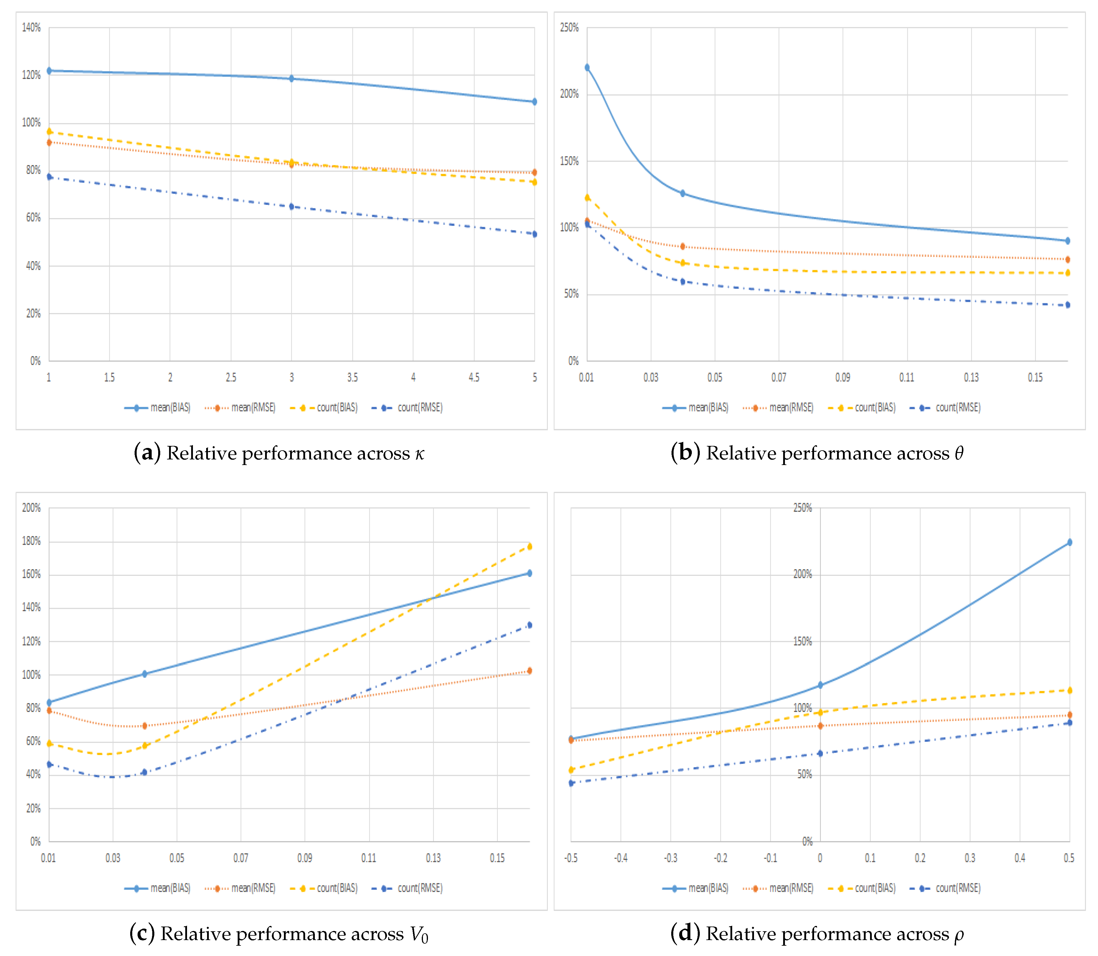
| Panel A: Across Mean Reversion | ||||||||
|---|---|---|---|---|---|---|---|---|
| Absolute Metrics | Counting Metrics | |||||||
| Regular Call | Symmetric Call | Regular Call | Symmetric Call | |||||
| Bias | RMSE | Bias | RMSE | Bias | RMSE | Bias | RMSE | |
| 1 | 0.0084 | 0.0139 | 0.0102 | 0.0128 | 0.5089 | 0.5638 | 0.4911 | 0.4362 |
| 3 | 0.0055 | 0.0099 | 0.0066 | 0.0082 | 0.5446 | 0.6063 | 0.4554 | 0.3937 |
| 5 | 0.0053 | 0.0093 | 0.0058 | 0.0074 | 0.5706 | 0.6516 | 0.4294 | 0.3484 |
| Panel B: Across Long-Term Variance | ||||||||
| Absolute Metrics | Counting Metrics | |||||||
| Regular Call | Symmetric Call | Regular Call | Symmetric Call | |||||
| Bias | RMSE | Bias | RMSE | Bias | RMSE | Bias | RMSE | |
| 0.01 | 0.0028 | 0.0077 | 0.0061 | 0.0081 | 0.4486 | 0.4938 | 0.5514 | 0.5062 |
| 0.04 | 0.0045 | 0.0084 | 0.0057 | 0.0072 | 0.5748 | 0.6241 | 0.4252 | 0.3759 |
| 0.16 | 0.0119 | 0.0170 | 0.0108 | 0.0130 | 0.6008 | 0.7037 | 0.3992 | 0.2963 |
| Panel C: Across Initial Variance | ||||||||
| Absolute Metrics | Counting Metrics | |||||||
| Regular Call | Symmetric Call | Regular Call | Symmetric Call | |||||
| Bias | RMSE | Bias | RMSE | Bias | RMSE | Bias | RMSE | |
| 0.01 | 0.0081 | 0.0115 | 0.0068 | 0.0090 | 0.6296 | 0.6818 | 0.3704 | 0.3182 |
| 0.04 | 0.0035 | 0.0088 | 0.0035 | 0.0062 | 0.6337 | 0.7051 | 0.3663 | 0.2949 |
| 0.16 | 0.0076 | 0.0128 | 0.0122 | 0.0131 | 0.3608 | 0.4348 | 0.6392 | 0.5652 |
| Panel D: Across Correlation | ||||||||
| Absolute Metrics | Counting Metrics | |||||||
| Regular Call | Symmetric Call | Regular Call | Symmetric Call | |||||
| Bias | RMSE | Bias | RMSE | Bias | RMSE | Bias | RMSE | |
| −0.5 | 0.0096 | 0.0120 | 0.0074 | 0.0092 | 0.6488 | 0.6927 | 0.3512 | 0.3073 |
| 0 | 0.0060 | 0.0105 | 0.0070 | 0.0092 | 0.5075 | 0.6008 | 0.4925 | 0.3992 |
| 0.5 | 0.0036 | 0.0105 | 0.0081 | 0.0100 | 0.4678 | 0.5281 | 0.5322 | 0.4719 |
| Panel A: Results across Number of Paths N | |||||||
|---|---|---|---|---|---|---|---|
| RMSE | Efficiency | Count | |||||
| Call | SCall | Optimal | Call | SCall | Call | SCall | |
| 20,000 | 0.0426 | 0.0178 | 0.0166 | 38.91% | 92.98% | 30.85% | 69.15% |
| 50,000 | 0.0480 | 0.0131 | 0.0125 | 26.00% | 95.56% | 20.00% | 80.00% |
| 100,000 | 0.0602 | 0.0104 | 0.0102 | 16.99% | 98.33% | 11.81% | 88.19% |
| 200,000 | 0.0540 | 0.0100 | 0.0100 | 18.49% | 99.95% | 2.34% | 97.66% |
| 500,000 | 0.0556 | 0.0124 | 0.0123 | 22.04% | 98.83% | 11.65% | 88.35% |
| Panel B: Results across Number of Regressors | |||||||
| RMSE | Efficiency | Count | |||||
| Call | SCall | Optimal | Call | SCall | Call | SCall | |
| 2 | 0.0832 | 0.0351 | 0.0345 | 41.41% | 98.17% | 10.14% | 89.86% |
| 3 | 0.0602 | 0.0104 | 0.0102 | 16.99% | 98.33% | 11.81% | 88.19% |
| 5 | 0.0201 | 0.0117 | 0.0099 | 49.34% | 84.48% | 60.99% | 39.01% |
| 9 | 0.0328 | 0.0154 | 0.0150 | 45.78% | 97.21% | 28.77% | 71.23% |
| 15 | 0.0625 | 0.0187 | 0.0184 | 29.39% | 98.00% | 24.45% | 75.55% |
| Panel A: Results across Number of Paths N | |||||||
|---|---|---|---|---|---|---|---|
| RMSE | Efficiency | Count | |||||
| Call | SCall | Optimal | Call | SCall | Call | SCall | |
| 20,000 | 0.1303 | 0.0163 | 0.0163 | 12.54% | 100.00% | 0.03% | 99.97% |
| 50,000 | 0.0986 | 0.0166 | 0.0166 | 16.81% | 100.00% | 0.22% | 99.78% |
| 100,000 | 0.0851 | 0.0157 | 0.0156 | 18.38% | 99.86% | 5.28% | 94.72% |
| 200,000 | 0.0590 | 0.0190 | 0.0185 | 31.36% | 97.52% | 21.22% | 78.78% |
| 500,000 | 0.0708 | 0.0106 | 0.0106 | 14.93% | 99.99% | 0.58% | 99.42% |
| Panel B: Results across Number of Regressors | |||||||
| RMSE | Efficiency | Count | |||||
| Call | SCall | Optimal | Call | SCall | Call | SCall | |
| 2 | 0.0983 | 0.0438 | 0.0437 | 44.42% | 99.63% | 6.78% | 93.22% |
| 3 | 0.0851 | 0.0157 | 0.0156 | 18.38% | 99.86% | 5.28% | 94.72% |
| 5 | 0.0498 | 0.0079 | 0.0079 | 15.79% | 99.03% | 7.97% | 92.03% |
| 9 | 0.0427 | 0.0091 | 0.0090 | 21.01% | 98.49% | 11.10% | 88.90% |
| 15 | 0.0458 | 0.0117 | 0.0116 | 25.36% | 99.36% | 7.90% | 92.10% |
| Panel A: Results for Individual Values of L | ||||||||||
|---|---|---|---|---|---|---|---|---|---|---|
| RMSE | Classified | Local Efficiency | Global Efficiency | |||||||
| L | Call | SCall | Optimal | RMSE | Picked | Efficiency | Call | SCall | Call | SCall |
| 2 | 0.0983 | 0.0438 | 0.0437 | 0.0437 | 93.34% | 99.83% | 44.42% | 99.63% | 7.45% | 16.72% |
| 3 | 0.0851 | 0.0157 | 0.0156 | 0.0157 | 95.36% | 99.65% | 18.38% | 99.86% | 8.61% | 46.79% |
| 5 | 0.0498 | 0.0079 | 0.0079 | 0.0079 | 95.74% | 99.66% | 15.79% | 99.03% | 14.72% | 92.27% |
| 7 | 0.0440 | 0.0082 | 0.0081 | 0.0081 | 96.77% | 99.78% | 18.36% | 98.31% | 16.65% | 89.17% |
| 9 | 0.0427 | 0.0091 | 0.0090 | 0.0090 | 97.44% | 99.90% | 21.01% | 98.49% | 17.15% | 80.41% |
| 11 | 0.0430 | 0.0100 | 0.0099 | 0.0099 | 97.89% | 99.96% | 22.92% | 98.85% | 17.02% | 73.40% |
| 15 | 0.0458 | 0.0117 | 0.0116 | 0.0116 | 99.17% | 99.99% | 25.36% | 99.36% | 16.01% | 62.75% |
| Panel B: Results for Multiple Values of | ||||||||||
| RMSE | Classified | Local Efficiency | Global Efficiency | |||||||
| Call | SCall | Optimal | RMSE | Picked | Efficiency | Call | SCall | Call | SCall | |
| All | 0.0379 | 0.0074 | 0.0073 | 0.0074 | 90.43% | 98.98% | 99.99% | 99.99% | 19.33% | 98.36% |
© 2019 by the author. Licensee MDPI, Basel, Switzerland. This article is an open access article distributed under the terms and conditions of the Creative Commons Attribution (CC BY) license (http://creativecommons.org/licenses/by/4.0/).
Share and Cite
Stentoft, L. Efficient Numerical Pricing of American Call Options Using Symmetry Arguments. J. Risk Financial Manag. 2019, 12, 59. https://doi.org/10.3390/jrfm12020059
Stentoft L. Efficient Numerical Pricing of American Call Options Using Symmetry Arguments. Journal of Risk and Financial Management. 2019; 12(2):59. https://doi.org/10.3390/jrfm12020059
Chicago/Turabian StyleStentoft, Lars. 2019. "Efficient Numerical Pricing of American Call Options Using Symmetry Arguments" Journal of Risk and Financial Management 12, no. 2: 59. https://doi.org/10.3390/jrfm12020059
APA StyleStentoft, L. (2019). Efficient Numerical Pricing of American Call Options Using Symmetry Arguments. Journal of Risk and Financial Management, 12(2), 59. https://doi.org/10.3390/jrfm12020059