Abstract
This study investigates the impact of exchange rate misalignment on outward capital flight in Botswana over the period 1980–2015. The study uses the autoregressive distributed lag (ARDL) approach to cointegration and the Toda and Yamamoto (1995) approach to Granger causality. Botswana’s currency misalignment was caused by current account imbalances. The most important determinant of capital flight from Botswana is trade openness, which indicates that exportable commodities are misinvoiced leading to net capital outflows. Our main findings show that in the long-run, when the currency is overvalued, the volume of capital flight through trade misinvoicing declines and increasing foreign reserves does not reduce outward capital flight. However, when the currency is undervalued, the volume of capital flight through trade misinvoicing increases and foreign reserves reduce outward capital flight. Investors respond more to prospects of devaluation than to inflation. Botswana should tolerate overvaluation of the pula of only up to 5%. When the pula is overvalued beyond 5%, capital flight increases substantially. The government has to formulate trade regulations and monitor imported and exported commodities. Botswana should also implement capital controls to limit capital smuggling and maintain monetary autonomy.
1. Introduction
Botswana is a small, upper middle-income economy in sub-Saharan Africa, dependent on its mining sector. Its principal export commodity is diamonds and prudent natural resource management policies have propelled its economy to grow significantly compared to other resource-rich countries. In addition, political stability is one of Botswana’s key features. Nonetheless, the country faces major economic problems. First, the capital-intensive mining sector has not reduced the persistent unemployment in Botswana. Second, the country has the third highest HIV prevalence in world, which increases fiscal pressures (Deléchat and Gaertner 2008; Hillboom 2008; Limi 2006; Matlho et al. 2019). In addition, previous studies indicate an important structural problem, namely, that Botswana’s currency (the pula) is overvalued (Iyke and Odhiambo 2016; Limi 2006; Pegg 2010; Taye 2012). Limi (2006) and Pegg (2010) indicate that the substantial mining revenue plays a role in this overvaluation. Lindgren and Wicklund (2018) posit that diamond prices and business confidence in Botswana have a negative correlation with the domestic exchange rate. Hence, the important issue considered in this study is the effects of exchange rate misalignment on the economy.
The extant literature shows that exchange rate overvaluation can increase capital flight, misallocate resources, abate economic efficiency and induce unfavourable downward spirals of trade and exchange rate controls (Cuddington 1986; Dornbusch 1984; Edwards 1989; Pfeffermann 1985; World Bank 1984). This study evaluates the impact of exchange rate misalignment on capital flight from Botswana over the period 1980–2015. The country aims to attract capital inflows to develop economic sectors other than mining. Botswana is unique because unlike other developing economies, it used only the fixed exchange rate regime since 1976. There has been no exchange rate regime change and the country has experienced significant undervaluation and overvaluation of the currency. It is conceivable that such misalignment has an impact on outward capital flight in Botswana. Botswana needs capital inflows for economic diversification, therefore, it is imperative to determine the impact of misalignment on capital flight from Botswana.
This study empirically investigates the impact of exchange rate misalignment on capital flight from Botswana. The examination contributes to the literature in two important ways. First, previous studies posit that the pula is overvalued but there is no study that evaluates the impact of exchange rate misalignment on capital flight from Botswana. The present study aims to fill this gap. The results of this study are important for implementing macroeconomic policies that support capital inflows for economic diversification in Botswana. Further, the World Bank (2019) indicates that Botswana’s diamond mines will be depleted by 2030. In the absence of diamonds, Botswana’s economic growth will decline drastically. Correcting exchange rate misalignment is necessary for early economic diversification and sustainable economic growth without diamonds.
Second, this investigation extends Gouider and Nouira (2014) methodological approach to misalignment. Gouider and Nouira (2014) defined overvaluation and undervaluation as either positive or negative misalignment without any thresholds. The lack of thresholds in Gouider and Nouira (2014) study implies that insignificant real effective exchange rate (REER) misalignments were included in the estimations. This study uses thresholds to capture only significant REER misalignment. This approach is important for determining which level of misalignment initiates high capital flight as an early warning indicator. This will curb substantial capital outflows, which are needed desperately for economic diversification in Botswana. The use of thresholds in this study allows policymakers to take informed actions in correcting misalignment, for example devaluing the currency. The results show that Botswana should tolerate overvaluation of the pula of only up to 5%. The present study uses the autoregressive distributed lag (ARDL) bounds testing approach to cointegration and the Toda and Yamamoto (1995) approach to Granger causality to determine the relationship between economic variables. This paper is organised as follows. Section 2 reviews the literature on exchange rate misalignment and capital flight. Section 3 presents the methodology used to achieve research objectives. Section 4 presents the results of the empirical models and discussions. Section 5 summarizes the results, reviews the objectives and provides policy implications. It also identifies areas for further investigation and study limitations.
2. Literature Review
The Smithsonian Agreement formulated in 1971 necessitated that developed nations should peg their currencies to the US dollar. The Nixon Shock caused the collapse of the Bretton Woods system of fixed exchange rates among developed nations. To stimulate economic growth by stabilising the real exchange rate (RER), developing economies subsequently adopted crawling pegs and managed floating regimes. In this regard, a major concern for economies engaged in trade is RER misalignment, which has economic growth implications. Misalignment is a common occurrence by which the RER deviates from the ideal or the equilibrium exchange rate. Fixed exchange rate regimes like Botswana are generally associated with exchange rate misalignment (Chowdhury and Wheeler 2015; Dubas 2009; Ghosh et al. 2015). Béreau et al. (2012) define exchange rate misalignment as the percentage gap between the observed exchange rate and the equilibrium real exchange rate (ERER). Deviations of the RER from the equilibrium instigated major currency crises in developing nations, such as the 1994 Mexican currency crisis, the 1997 Asian currency crises and the 1999 Brazilian financial crisis. Currencies of Asian economies were significantly misaligned before the currency crisis (Chinn 2000; Coudert et al. 2013; El-Shagi et al. 2016; Jeong et al. 2010; Kinkyo 2008).
The literature posits that overvaluation of the RER was the cause of capital flight in Latin America (Cuddington 1986). The Latin American debt crisis was a financial crisis accompanied by significant capital flight. The debate as to whether capital flight initiated the debt crisis or foreign debt caused capital flight in Latin America is ongoing. Capital flight occurs when monetary assets flow out of a country rapidly as a response to economic and political changes. It leads to loss of wealth and depreciation of the local currency. Erbe (1985) defines capital flight as total private capital outflows from developing nations. Dooley (1986) and Lessard and Williamson (1987) suggest that capital flight should be distinguished by its motivations rather than economic consequences. A challenge facing research on capital flight is its measurements, which do not capture the actual value of capital flight because capital flight can occur illegally. Illegal capital outflow is large in developing economies since they have ineffective, or no capital controls to stimulate foreign direct investment (FDI) inflows. Capital flight has significant adverse effects on economic growth, particularly in developing economies, because it reduces private and public investment. As capital leaves the domestic economy, government tax revenue declines, which reduces funding for public investments. Therefore, the government must borrow from foreign bodies at high costs. The interest rate for an investor taking assets abroad is fixed. However, the loan interest incurred by the government increases with the magnitude of the loan. Hence, capital flight creates major debt obligations, particularly in developing economies (Cuddington 1986).
According to Hermes et al. (2004), capital flight occurs owing to macroeconomic instability and manifests in multiple ways, such as budget deficits, current account deficits, overvaluation of the currency and high inflation. Overvaluation of the domestic currency is an important underlying determinant of capital flight. Expectations of depreciation are high when the currency is overvalued. Since investors aim to maximize returns and avoid welfare losses, domestic investors would be inclined to send their monetary assets abroad. The literature on exchange rate misalignment argues the Botswana pula is overvalued because of mining revenue (Limi 2006; Pegg 2010). Hence, this study aims to identify the impact of exchange rate misalignment on capital flight from Botswana as an attempt to promote FDI inflows, economic diversification and sustainable growth.
Few studies investigate the effects of exchange rate misalignment on capital flight. To determine these effects, we have to reflect on the exchange rate expectations theory developed by Hermes et al. (2004). The theory posits that an overvalued currency leads to increasing expectations of depreciation in the future. As a result, economic agents will demand more foreign goods than domestic goods, leading to inflationary pressures and loss of real income. Under such circumstances, economic agents will prefer to hold their assets abroad to avoid welfare losses, leading to capital flight. Gouider and Nouira (2014) examine the role of exchange rate misalignment on capital flight for a sample of 52 developing economies using data on the 1980–2010 period. Their results show that strong undervaluation of the domestic currency restricts capital flight, while strong overvaluation stimulates it (Gouider and Nouira 2014). Further, Sohrabji (2011) examines the link between capital flows and REER overvaluation. The author uses Edwards’ (1989) model, cointegration tests and an error-correction model. The results show that capital inflows significantly contribute to exchange rate misalignment.
Botswana has no exchange rate restrictions, since it aims to boost domestic business efficiency and FDI inflows. The country attracted significant capital flows in the mining sector with moderate portfolio investments (Bank of Botswana 2016). FDI in Botswana is required for investment capital, economic diversification and promotion of inclusive growth. In 2017, Botswana experienced loss of foreign exchange reserves due to appreciation of the pula, which increases its exposure to a financial crisis (Agénor et al. 1992; Coudert et al. 2013; El-Shagi et al. 2016; Jeong et al. 2010; Kaminsky et al. 1998; Kinkyo 2008; Krugman 1979). Following Hermes et al. (2004) and Cuddington (1986), overvaluation of the pula may create expectations of depreciation thereby increasing capital outflows. The central bank conducted portfolio-rebalancing operations in 2017 to counter persistent capital outflows. As regards the literature on this issue, although capital inflow is vital to Botswana’s economy, previous studies have not evaluated the impact of exchange rate misalignment on capital flight from Botswana.
3. Methodology
This section explains the methodology used to determine the relationship between exchange rate misalignment and capital flight from Botswana. It provides research hypotheses and estimation approaches as well as diagnostic measures. According to Edwards (1989), exchange rate misalignment causes severe welfare and efficiency costs owing to exchange rate and trade controls that accompany overvaluation. There is supporting evidence that REER misalignment reduces exports and deteriorates the agricultural sector (Pfeffermann 1985; World Bank 1984). A financial risk associated with exchange rate misalignment is that it generates massive capital flight, which increases social welfare costs (Cuddington 1986). Anticipations of macroeconomic instability cause high capital outflows, inducing large, rapid adjustments in interest rates and exchange rates. Further, capital flight reduces the tax base and this reduction increases budget deficits and costs of foreign borrowing (Cuddington 1986; Dornbusch 1984; Edwards 1989).
Previous studies posit that overvalued currencies generate capital flight (Cuddington 1986; Edwards 1989; Gouider and Nouira 2014; Pastor 1990). As Hermes et al. (2004) describe, overvaluation of the REER creates expectations of depreciation of the domestic currency, thereby increasing capital outflows. Currency devaluation diminishes the value of domestic assets relative to foreign assets, which encourages residents to switch to foreign assets (Cuddington 1986; Dornbusch 1984; Lessard and Williamson 1987). However, an increase in foreign exchange reserves allows the government to prevent balance of payments crises and macroeconomic crisis (Alam and Quazi 2003). As a result, investor confidence in the economy is boosted, which reduces capital outflows (Boyce 1992). Thus, the literature shows that exchange rate misalignment and capital flight affect a country’s economic stability and growth. Hence, to examine these effects in relation to Botswana, this study proposes the following hypotheses:
H1.
Overvaluation of the pula increases capital flight in the long-run.
H2.
Undervaluation of the pula decreases capital flight in the long-run.
To determine the impact of exchange rate misalignment on capital flight, Botswana’s exchange rate fundamentals should be identified first. Exchange rate fundamentals are variables that determine the REER and thus the internal and external equilibrium of the economy (Edwards 1989). Edwards (1988) proposes that exchange rate fundamentals in developing economies are terms of trade, government consumption, technological progress and capital inflows. However, further research on exchange rate misalignment shows that other macroeconomic factors, such as external debt, trade openness and capital formation are important determinants of the REER (Gouider and Nouira 2014; Hossain 2011; Pham and Delpachitra 2015; Salim and Shi 2019). Following Edwards (1988) and Hossain (2011), the relative impact of the exchange rate fundamentals for Botswana is specified as follows:
The definition of terms is as follows. (dependent variable) is the natural log of the REER index. is the natural log of the terms of trade index. is the natural log of government final consumption expenditure. is the rate of GDP growth to measure domestic technological progress. is FDI net capital inflows. is the real official foreign aid inflow received by Botswana. is the natural log of trade openness. is the natural log of Botswana’s stock of external debt. is the natural log of the domestic gross capital formation. The epsilon represents the error term (Table S1).
To evaluate the degree of misalignment, first, the long-run exchange rate fundamentals for the Botswana economy are determined using Equation (1). Next, the Hodrick–Prescott (HP) filter is used to separate permanent and temporary components of the exchange rate fundamentals to obtain the long-run values (HP trend). Hodrick and Prescott (1997) used this technique to analyse post-war business cycles. The filter computes the smoothed series, of by minimising the variance of around . The filter uses to minimise the equation:
Consequently, the long-run exchange rate fundamentals are used to estimate the long-run . The fitted is filtered to obtain the equilibrium REER . The smoothness of the series is determined using the parameter . Since this study uses annual data, the optimal value1 for is 100. The next step is to calculate the degree of misalignment as follows:
The next phase is to evaluate whether misalignment of the pula was caused by unsustainable fiscal and monetary policies following Hossain (2011). The Toda and Yamamoto (1995) approach to Granger causality is applied to determine causation between the REER misalignment , cyclical components of the current account , external debt and real GDP . Excess broad money supply is captured by the variable . The cyclical component will be derived from the filtered series . is the natural log of real GDP. The cyclical component will be obtained from the filtered natural log of (100 + ) where is the total stock of external debt as a percentage of GDP. is excess broad money supply defined as the difference between actual broad money supply and the predicted broad money supply. Owing to data limitations, the broad money determinants used are Botswana’s real GDP and the annual yield on the US government medium-term bond . The cyclical component will be obtained from the filtered natural log of (100 + ) where is the current account balance as a percentage of GDP.
Following Gouider and Nouira (2014), this study decomposes misalignment into overvaluation and undervaluation . will take the positive values of the misalignment, while will be negative misalignment. As a contribution to the literature, a 5% threshold2 for misalignment is set to capture only significant deviations from the equilibrium real effective exchange rate (EREER). Therefore, from Equation (3), and are defined as:
To determine the impact of exchange rate misalignment on capital flight from Botswana, this study will adopt the exchange rate expectations theory developed by Hermes et al. (2004). The theory posits that an overvalued currency leads to increasing expectations of depreciation in the future. Hence, economic agents will demand more foreign goods than domestic goods, leading to inflationary pressures and loss of real income. Under such circumstances, economic agents will prefer to hold their assets abroad, leading to capital flight. The principal methods used for measuring capital flight in the extant literature are the residual method, the Dooley method and the hot money approach. Hermes et al. (2004) argue that the Dooley and hot money methods provide inaccurate estimates of capital flight. This study adopts the residual method to estimate the volume of capital flight3 from Botswana. This method evaluates capital flight by comparing sources of capital flows and their use in the economy. An advantage of this approach is that it measures all private capital outflows as capital flight (Hermes et al. 2004). Following Hermes et al. (2004), capital flight from Botswana will be estimated as follows:
is Botswana’s current volume of outward capital flight (monetary value) not scaled to GDP. is the first difference of Botswana’s stock of gross external debt. is the net foreign investment inflows in Botswana. is Botswana’s current account deficit and is the first difference of the stock of official foreign reserves. Following Alam and Quazi (2003), Ndikumana and Boyce (2003) and Cheung and Qian (2010) an econometric model for capital flight based on the determinants is specified as:
The definition of the variables is as follows. (dependent variable) is the volume of Botswana’s outward capital flight4 as a percentage of GDP. Note that this variable is different from which is the monetary value of Botswana’s outward capital flight. The variable is better than because it facilitates tracking of the dynamics of capital flight from the Botswana economy. The regressors are defined as follows. is the volume of reserves per GDP. is the real GDP growth rate. is the domestic inflation rate. is the real interest rate differential5 between Botswana and South Africa due to proximity and economic linkages between the two countries (Kganetsano 2007).6 is the real foreign aid inflow. is the natural log of trade openness. is the natural log of external debt. is natural log of the REER index for Botswana. The epsilon represents the error term.
Equation (7) does not directly assess the impact of REER misalignment, which is the focus of this investigation. To determine the effects of misalignment on capital flight, in Equation (7) is substituted with overvaluation and undervaluation dummies as follows:
3.1. Time Series Properties and Estimators
The long-run relationship between variables in levels can be evaluated using the Engle–Granger two-step residual based procedure (Engle and Granger 1987) and Johansen’s system-based reduced rank regression approach (Johansen 1988; Johansen and Juselius 1990). A disadvantage of the Engle and Granger (1987) approach is the small sample bias arising from the exclusion of short-run dynamics (Alam and Quazi 2003). The procedures developed by Johansen (1988) and Phillips and Hansen (1990) require that the variables involved should be . However, the ARDL bounds testing procedure developed by Pesaran et al. (2001) applies whether the regressors are , purely or integrated of different orders. Hence, this study adopts the ARDL bounds testing procedure to examine REER misalignment and capital flight from Botswana (Equations (1), (8) and (9)). The bounds testing procedure is advantageous since it can be executed even if the explanatory variables are endogenous. The approach is also suitable for smaller samples. To perform the bounds test, the following steps are followed. First, we determine the stationarity of the variables. Then, the optimal lag for the model is evaluated using the Schwarz–Bayesian information criterion (SBIC). The long-run relationship between the variables in levels is evaluated using the bounds test. Following Pesaran et al. (2001), the error correction models for this study are represented as:
The definition of terms is as follows. is the first difference operator. is the regression constant while represents the white noise error term. indicate the long-run coefficients while represent the error correction short-run dynamics. The error-correction models for the above equations after affirming the long-run relationship between the variables is specified as follows:
where the term is the error-correction term and is its coefficient. The term represents the speed of convergence to the equilibrium level if there is a disturbance in the system.
This study further uses the Toda and Yamamoto (1995) approach to Granger causality to investigate the causal relationship among the variables. The ordinary Granger causality test is not suitable for this investigation since the variables under investigation are not all . Further, Wolde-Rufael (2005) argue that the F-statistic in Granger causality may be invalid because the test lacks a standard distribution in cases where the times series is cointegrated. An advantage of the Toda and Yamamoto (1995) approach is its applicability whether a series is non-cointegrated or cointegrated of different arbitrary orders. The test also uses a modified Wald test and a standard autoregressive model in levels form to reduce the likelihood of mistakenly identifying the order of the series (Mavrotas and Kelly 2001). For estimation purposes, the vector autoregression (VAR) system for and the causes of misalignment is represented as:
where is any of the potential causes of misalignment and . The VAR system represents the bivariate relationship between and each potential cause. The causal links examined are as follows: and . The highest order of integration is denoted by . Likewise, the VAR system for and its causes, is represented as:
where is any of the determinants of . The VAR system represents the bivariate relationship between and each potential cause. The bivariate causal links examined are as follows:
3.2. Data Diagnostics
This investigation uses annual data (time series) for the Botswana economy for the period 1980–2015. The data sources are the International Financial Statistics (IFS), World Development Indicators (WDI) and the Federal Reserve Economic Data (FRED). The study adopts the ARDL bounds testing approach, which is applicable whether all the regressors are or or a mixture of both. However, the procedure is not valid if any of the variables under examination is . This investigation used the generalised least squares transformed Dickey–Fuller (DF-GLS) test and the augmented Dickey–Fuller (ADF) unit root test to examine stationarity. An advantage of the DF-GLS procedure is that it has high power even when the root of the times series is closer to unity (Elliot et al. 1996). The results of the tests showed that the sample is a mixture of and series. Multicollinearity was assessed using the variance inflation factor (VIF) in this study. As a rule of thumb, VIFs greater than 10 signal a serious multicollinearity problem while VIFs between 5 and 10 signal a less serious problem of multicollinearity (Pedace 2013). The VIFs for the variables in this investigation are less than 6, which is acceptable for further analysis.
4. Results
This section reports and discusses empirical findings on exchange rate misalignment in Botswana. First, it investigates the determinants of Botswana’s REER using the ARDL approach to cointegration. Next, based on the exchange rate fundamentals, the EREER is estimated to evaluate the degree of misalignment. Lastly, the Toda and Yamamoto (1995) approach to Granger causality is used to investigate causal relations between REER misalignment and its potential causes. Granger (1981), Engle and Granger (1987) and Johansen (1988) pioneered the use of cointegration for time series analysis. Following Engle and Granger (1987), a series without a deterministic component but with a stationary autoregressive moving average after differencing times is integrated of order , []. The properties of and series differ based on their responsiveness to innovations. If , its variance is finite and innovations have a short-term effect on the magnitude of . In contrast, an innovation has a long-term effect on the value of an series (Engle and Granger 1987). The procedure followed for the ARDL bounds cointegration approach is as follows. First, the variables were subjected to stationarity tests. The results show that only is while other variables and are . Next, the optimal lag length of the specifications is determined using the SBIC. The SBIC is used to determine the optimal lag length since it is more reliable for optimal model selection than the Akaike information criterion (AIC) (Pesaran and Shin 1999). The long-run levels relationships for different specifications are evaluated using the F-test. Subsequently, the coefficients of the variables are estimated with diagnostic tests.
The benchmark for determining a long-run relationship between the dependent variable and independent variables is the F-test. The optimal lag established for the ARDL model using the SBIC is zero when is the dependent variable. The null hypothesis of no cointegration is against the alternative . The criterion for the long-run equilibrium relationship is based on the lower and upper bound critical values proposed by Pesaran et al. (2001). Following Pesaran et al. (2001), we reject the null of no long-run equilibrium relationship if the computed F-statistic is higher than the upper bound critical values. However, if the F-statistic is less than the lower bounds, we fail to reject the null of no long-run equilibrium relationship. The test is inconclusive if the F-statistic falls between the lower and upper bounds.
Banerjee et al. (1998) suggest that a negative and significant error-correction term signals a long-run relationship. The F-test for the parameter that in the specification with as the dependent variable is expressed as where to are the determinants of the REER. The procedure is repeated by interchanging the dependent variable with the regressors. The order of the variables when is an independent variable is . Following Pesaran et al. (2001) we determine the F-test by including a restricted constant (RC); unrestricted constant (UC) and unrestricted constant with unrestricted trend (UC + UT) in the specifications. This is important because it helps to determine the sensitivity of the long-run equilibrium relationship to a deterministic trend. When a specification includes RC, it indicates the dynamics of the long-run equilibrium relationship when the intercept is restricted with no linear trend. When a specification includes UC it shows the dynamics of the relationship when an unrestricted constant with no trend is included in the specification. Consequently, when a specification includes UC + UT it reveals the relationship between the variables when there is an unrestricted constant with unrestricted trend in the model specification. Since with trend and intercept (Table 1) is greater than the upper limit of the critical bound (3.23 > 3.14), the null hypothesis of no long-run equilibrium relationship7 is rejected at the 10% level. In addition, when the test is conducted with restricted and unrestricted constants, the null of no long-run equilibrium relationship is rejected at the 5% level. Further, when is switched to a regressor position, the computed F-statistic for the majority of the determinants of the REER is greater than the upper bound critical values indicating a long-run equilibrium relationship. The presence of a long-run equilibrium relationship indicates that the regressors are not long-run forcing variables8 (Pesaran et al. 2001). Table 1 presents the results of the F-test.

Table 1.
Results of the F-test for the long-run relationship between the real effective exchange rate (LNREER) and its determinants.
The next phase of the ARDL cointegration approach is to estimate the coefficients of the exchange rate fundamentals. The ARDL technique estimates number of regressions for the optimal lag length for each variable. The term is the maximum number of lags and here is the number of variables in the equation. The optimal SBIC lag length is zero while that for AIC is one. Since a small lag length provides better results, the optimal lag used was zero. AIC selected the same model as SBIC (1, 0, 0, 0, 0, 0, 0, 1, 0). The estimated error-correction model is robust since the short-run coefficients were significant. The diagnostic tests did not indicate autocorrelation, endogeneity, non-normality of the residuals or heteroskedasticity. Further, the CUSUM plots were within the 5% boundaries, indicating no systematic change of the estimated coefficients. To obtain a parsimonious model, the Wald test was used to test for the significance of the coefficients of the unrestricted model. The variables and were deleted and the restricted model was estimated with the remaining variables. Table 2 and Table 3 presents the results of the restricted model.
Table 2.
Long-run coefficients of the determinants of LNREER (restricted model).
Table 3.
Error-correction model (restricted model).
This section discusses the results of the restricted model (Table 2). The coefficient for terms of trade is statistically significant with a negative sign (−0.3551), which indicates that improvements in terms of trade terms increases the demand for foreign goods, resulting in REER depreciation. This finding is not consistent with that of Hinkle and Montiel (1999), who argue that improvements in terms of trade appreciate the REER for imports by increasing the demand for non-tradables. In the case of Botswana, an improvement in terms of trade reflects a higher demand for mineral exports. The revenue generated is used to purchase more imports (food, fuel and machinery), typically from South Africa.9 Approximately 80% of Botswana’s imports originate from South Africa. This causes a high demand for the foreign currency, resulting in REER depreciation. The coefficient for is negative (−0.0038) and not significantly different from zero, which signals low technological progress in Botswana and a minor impact on the REER. The negative coefficient is not consistent with the Balassa–Samuelson effect, which stipulates that a high rate of technological progress will cause an equilibrium REER appreciation (Balassa 1964; Gouider and Nouira 2014; Samuelson 1964). The coefficient is negative since the manufacturing sector in Botswana is small and unable to meet technological demands of the large mining sector. Attempts to diversify the economy have been unsuccessful because the manufacturing and agriculture sectors have not grown significantly. The manufacturing sector contributes approximately 6% to GDP while the mining sector contributes nearly 25%. Machinery and equipment are imported from other countries and less is spent on domestic non-tradable goods. The demand for foreign currency causes the depreciation of the pula.
The coefficient for inflows is negative and statistically significant (−0.0193) indicating that received increases the demand for importable commodities relative to domestic goods, which depreciates the REER. This result deviates from the findings of Alam and Quazi (2003), who argued that the supply of foreign aid induces currency appreciation. This result can be explained by the rapid development of the mining sector in Botswana because aid received was used to purchase mining machinery and equipment abroad. The government also solicited foreign expertise to develop physical and social infrastructure. Therefore, less aid was spent on the small non-tradable goods market. This results in the depreciation of the REER. The coefficient for is positive and statistically significant (0.2374), which signals that removing trade barriers results in a higher demand for domestic goods, including non-tradables, leading to REER appreciation. This result is not in line with the theory that trade liberalisation reduces the demand for non-tradables goods, which depreciates the REER (Gouider and Nouira 2014). The positive coefficient can be explained by Botswana’s membership of the Southern African Customs Union (SACU)10. Other member states are Lesotho, Namibia, South Africa and Swaziland. The SACU agreement is based on the promotion of free movement of goods between the territories of the member economies. Trade liberalisation increases the external demand of Botswana’s goods. The public in Botswana will subsequently increase their expenditure on the non-tradable commodities, resulting in REER appreciation. The variable has a negative and significant coefficient (−0.0553), signifying that a depreciating pula is necessary for financing high external debt. The result is consistent with that of Hossain (2011), who found that an increase in foreign debt in Bangladesh required depreciation of the taka for debt financing.
The variable holds a positive coefficient (0.0462), which signals that a high level of capital accumulation in Botswana increases expenditure on non-tradable goods, which appreciates the REER. This result is inconsistent with the findings of Pham and Delpachitra (2015), who argue that capital stock and investment cause a depreciation of the REER. Improvements in accumulated capital are more likely to increase productivity. The positive relationship can be explained by programmes introduced by the Botswana National Productivity Centre, which encourage productivity and sustainable performance. The Enterprise Support Programme and the Public Service Programme were established to improve performance and productivity in the private and public sectors. The central bank also encourages sustained improvements in productivity, to reduce inflation in Botswana. The acquisition of capital improves productivity, which results in a higher supply and consumption of non-tradable commodities. This eventually leads to REER appreciation.
The signs of the variables in the error-correction model are consistent with those of the long-run coefficients. The sign and the magnitude of the error-correction term is important for evaluating the short-term adjustment process. A positive value of will cause to diverge from its long-run equilibrium path in relation to exogenous-forcing variables. The coefficient for the error-correction term is −0.6869 (Table 3) and is significant at the 1% level, which suggests that tends to cause to converge monotonically to its long-run equilibrium path at a speed of 68.69% annually. The negative and significant error-correction term further validates the long-run equilibrium relationship between and its associated determinants.
Based on the long-run coefficients of the restricted model (Table 2), Botswana’s exchange rate fundamentals are and . The long-run values of the exchange rate fundamentals and the EREER were obtained using the HP filter. The pula seems to have experienced misalignment, calculated by the deviation of from . Figure 1 shows the degree of misalignment.
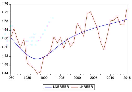
Figure 1.
Botswana pula misalignment (1980–2015).
The two types of exchange rate misalignment are macroeconomic-induced misalignment and structural misalignment. In theory, the former is prompted by inconsistent fiscal and monetary policy. In contrast, structural misalignment arises when exchange rate fundamentals are not reflected into changes of the REER. In developing economies such as Botswana, it is common for exchange rate misalignment to occur owing to inconsistent fiscal and monetary policies. This section evaluates whether misalignment of the pula was caused by unsustainable fiscal and monetary policies. The Toda and Yamamoto (1995) approach to Granger causality is applied to determine causation between REER misalignment , cyclical component of the current account , cyclical component of external debt , cyclical component of real GDP and excess broad money supply . The ADF test indicates that only is while and are . Following Wolde-Rufael (2005), the procedure is to augment the correct VAR order , by the highest order of integration . The next step is to estimate a order of the VAR. Serial correlation of the residuals was evaluated using the Breusch–Godfrey serial correlation LM test. The null hypothesis of no serial correlation was not rejected for all the tests. The data span is from 1980 to 2015 for all series. Table 4 presents the results of the causality test.
Table 4.
Causality between MISREER and its potential causes.
Drawing from the results of the causality test, Botswana’s REER misalignment is caused by the cyclical component of the current account. This indicates that REER misalignment is caused by current account imbalances. Further, REER misalignment had a significant influence on Botswana’s current account balance as shown by the reverse causality effect from REER misalignment to the cyclical component of the current account. There is no evidence of causality between REER misalignment and external debt and REER misalignment and excess broad money supply. This finding signals that exchange rate misalignment in Botswana was not caused by inconsistent fiscal and monetary policies. In addition, there was no evidence of causality between misalignment and the cyclical component of real GDP, revealing that REER misalignment had no significant impact on economic growth in Botswana.
4.1. The Causes of Capital Flight from Botswana
Before examining the impact of REER misalignment on capital flight, we have to determine the causes of capital flight from Botswana. Botswana experienced a high level of capital flight between the years 1980 and 1985 (see Figure A1 in the Appendix A). In 1980, capital flight amounted to 24.75% of GDP. The magnitude of capital flight declined to 2.05% of GDP in 1985. Between 1986 and 2000, Botswana experienced inward capital flight, which indicates the rapid development of the mining sector. In 2007, Botswana experienced inward capital flight of 16.35%, which declined drastically to 0.89% as outward capital flight in 2008. This marks the period of the 2007−2008 Global Financial Crisis as investors were seeking higher returns for their monetary assets in other economies. The general trend is that from 2012 to 2015, Botswana experienced increasing inward capital flight amounting to 6.34% of GDP in 2015. This may be attributed to the Sectoral Development and Business Linkages Unit developed in 2011, which was designed to attract FDI and promote skills transfer as part of the Economic Diversification Drive. On average, Botswana experienced inward capital flight over the period 1980−2015.
The general to specific approach is used to identify determinants of capital flight. Trade openness and the level of foreign reserves are found to be the determinants of Botswana’s capital flight. The other variables and are redundant and have no explanatory power on capital flight from Botswana. The results of the stationarity tests show that the variable is while and are . The F-test as described by Pesaran et al. (2001) is used for determining a long-run relationship for the variables and . The optimal lag established for the ARDL model using the SBIC is zero when is the dependent variable. The null hypothesis of no long-run equilibrium relationship is whereas the alternative is . The F-test for the restriction that when is the dependent variable is expressed as . The process is repeated by interchanging the dependent variable with the regressors. The F-statistic for with trend and intercept is greater than the upper limit of the critical bound (22.23 > 7.52). Consequently, the null hypothesis of no long-run equilibrium relationship is rejected at the 1% significance level. The test is also executed with constants only and the null of no long-run equilibrium relationship is still rejected at the 1% significance level. The null hypothesis of no long-run equilibrium relationship is rejected at the 5% level when is a dependent variable in all regressions. However, the variable indicated no evidence of a long-run equilibrium relationship with other variables when it is a dependent variable.
The next procedure is to estimate the short-run and long-run coefficients for and . The optimal lag length for SBIC and AIC is zero when is the dependent variable. AIC selected the same model as SBIC (1, 0, 1). Table 5 presents the results of the estimated coefficients.
Table 5.
Coefficients of the determinants of capital flight (KF).
The estimated error-correction model is robust since the short-run coefficients are significant. The diagnostic tests do not signal autocorrelation, endogeneity, non-normality of the residuals or heteroskedasticity. The estimated model is stable because the CUSUM plots suggested no systematic changes in the estimated coefficients. The coefficient for is positive and significant (62.3474), which signals that trade liberalisation increases the volume of outward capital flight. The coefficient suggests that the reported value of Botswana’s exports is understated, leading to net capital outflows through trade. According to Global Financial Integrity (Global Financial Integrity 2015), Botswana lost approximately 13 billion US dollars through trade misinvoicing in 2004–2013. The estimated value of Botswana’s under-invoiced exports is approximately 9 billion US dollars against 4 billion US dollars for over-invoiced exports during 2004–2013 (Global Financial Integrity 2015). In the case of imports, the disparity was small, which indicates that the economy experiences net capital outflows through trade. Ajayi and Ndikumana (2015) posit that trade misinvoicing occurs by understating the quantity of goods or prices. The seller sends the difference between the actual earnings and the understated values to foreign accounts. The results are consistent with those of Cheung and Qian (2010), who argue that increasing trade openness allows economic agents to falsify trade prices in China, resulting in a rise in capital flight.
The coefficient for is negative and statistically significant (−0.7727) indicating that a high level of foreign reserves11 reduces outward capital flight. An increase in reserves indicates that the central bank can intervene in the foreign exchange market to stabilise the local currency’s exchange rate, which reduces capital outflows. In addition, a high level of reserves indicates that the government can finance current account deficits by selling foreign currency in the foreign exchange market. This finding is consistent with that of Boyce (1992), who asserts that a higher level of reserves indicates a lower probability of a balance of payments crisis,12 which reduces capital flight. The results of the error-correction model show that only was not significant in the short-run. The coefficient for is positive with a lesser impact (9.9306) than the long-run coefficient (62.3474). This shows that trade misinvoicing is a process that intensifies over time. The value for the error-correction term = −0.4705) is significant at the 1% level, which indicates a speed of convergence to equilibrium at 47.05% per annum. The statistical significance and the negative sign of the error-correction term confirm the presence of a long-run equilibrium relationship between and .
The previous section indicated that trade openness and the level of foreign reserves are the determinants of capital flight from Botswana. The aim of the following sections is to examine the effects of exchange rate misalignment on capital flight by including dummy variables for overvaluation and undervaluation in the specification.
4.1.1. The Impact of Overvaluation on Capital Flight
The null of the first hypothesis proposed that overvaluation of the Botswana pula increases capital flight in the long-run. In this study, a 5% threshold for positive misalignment was used to create the overvaluation dummy variable . The variable is included in the regression to determine its effect on capital flight and other regressors. The F-test is used to determine a long-run relationship between and . The optimal lag established for the ARDL model using the SBIC is zero when is the dependent variable. The computed F-statistic when is the dependent variable with trend and intercept is greater than the upper limit of the critical bound (16.10 > 6.36). The null hypothesis of no long-run equilibrium relationship is rejected at the 1% significance level. The test is performed again with constants only and the null of no long-run equilibrium relationship is still rejected at the 1% significance level. The null hypothesis of no long-run equilibrium relationship is rejected at the 1% significance level when is a dependent variable in all cases. However, when the variables and are dependent variables, the null hypothesis of no long-run equilibrium relationship is not rejected in all cases. The optimal lag length for SBIC and AIC is zero when is the dependent variable. AIC selected the same model as SBIC (1, 0, 0, 1). Table 6 presents the results of the estimated regression coefficients.
Table 6.
Estimated coefficients of the overvaluation dummy (OVER) and other determinants of KF.
The estimated error-correction model above shows no challenges of endogeneity, non-normality of the residuals or heteroskedasticity. The estimated coefficients for the model are systematically stable. The coefficient for is positive (8.0067), indicating that an overvalued currency leads to increasing expectations of depreciation in the future resulting in substantial capital outflows13. Consequently, we fail to reject the null of . The results are consistent with those of Cuddington (1986), who shows that overvaluation of the Argentine Peso increased the probability of a major devaluation and was the cause of capital flight in 1980–1982. The coefficient for is positive and significant (49.3755) at the 5% significance level. This signals that when the currency is overvalued, trade liberalisation increases the volume of outward capital flight through exportable commodities. This finding is consistent with that of Cheung and Qian (2010).
The coefficient for is positive (0.2439), indicating that increasing the level of foreign reserves when the currency is overvalued does not reduce outward capital flight. This result is not consistent with that of Boyce (1992), who argues that a higher level of reserves reduces capital flight. This finding can be explained by Botswana’s history of devaluation of the pula for competitiveness of exports. The pula was devalued seven times between 1980 and 2005. The highest devaluation was 15% in 1985 and 12% in 2005. Investors may expect a larger depreciation of the pula, leading to high capital outflows. The fear of welfare losses from devaluation may be too high such that increasing foreign reserves does not deter investors from sending their assets abroad.
The results of the error-correction model show that only was significant in the short-run. The coefficient for is positive with a lower impact (27.7653) than the long-run coefficient (49.3755). This is because in the long-run, economic agents involved in trade misinvoicing have more experience, leading to higher capital outflows than in the short-run. In the short-run, still bears a positive sign (4.4302), indicating that overvaluation increases capital flight. The value for the error-correction term = −0.6547) is significant at the 1% significance level, which signals a speed of convergence to equilibrium at 65.47% annually. The statistical significance and the negative sign of the error-correction term further confirm the presence of a long-run equilibrium relationship between and .
4.1.2. The Impact of Undervaluation on Capital Flight
The null of the second hypothesis proposed that undervaluation of the Botswana pula decreases capital flight in the long-run. Similar to the procedure followed to determine overvaluation, a 5% threshold is used to create the undervaluation dummy variable . The F-test is used to determine a long-run relationship between and . The optimal lag established for the ARDL model using the SBIC is zero when is the dependent variable. The computed F-statistic when is the dependent variable with trend and intercept is greater than the upper limit of the critical bound (25.38 > 6.36). The null hypothesis of no long-run equilibrium relationship is rejected at the 1% significance level. When the variable is a dependent variable, the null hypothesis of no long-run equilibrium relationship is rejected at the 5% level in all regressions (RC, UC and UC + UT). However, when and are dependent variables, the null of no long-run equilibrium relationship is not rejected. The optimal lag length for SBIC and AIC is zero when is the dependent variable. Table 7 presents the results of the estimated regression coefficients.
Table 7.
Estimated coefficients of the undervaluation dummy (UNDER) and other determinants of KF.
The estimated error-correction model (Table 7) shows no problems of serial correlation, endogeneity, non-normality of the residuals or heteroskedasticity. The model is systematically stable as its CUSUM plots were within the 5% boundaries. The coefficient for is positive (3.8561), indicating that an undervalued currency increases outward capital flight. Consequently, we reject the null hypothesis of . The results are not consistent with the findings of Gouider and Nouira (2014), who argue that undervaluation has no effect on capital flight. This disparity can be explained by the methodology Gouider and Nouira (2014) used. The duo did not use any threshold for determining undervaluation. Undervaluation was assumed as cases where the calculated value for misalignment was negative. Therefore, the study included redundant observations in the analysis that may not qualify to be undervaluation. In the present study, a 5% threshold is used to capture only significant cases of undervaluation14. The results agree partially with those of Gouider and Nouira (2014) because the Chi-square statistic p-value (p = 0.5014) for the variable indicates that undervaluation is a minor determinant of capital flight. Therefore, for a restricted model, the variable can be deleted.
The coefficient for is positive and significant (64.0550) at the 5% significance level. This signals that when the currency is undervalued, removing trade barriers increases the volume of outward capital flight through exportable commodities. The coefficient for when the currency is undervalued is greater than when the currency is overvalued (64.0550 > 49.3755). This can be explained by an increase in the volume of exports when the currency is undervalued (Vo et al. 2019; Thuy and Thuy 2019). An undervalued currency raises competitiveness of exports, which allows more goods to be misinvoiced and results in high capital flight. However, when the currency is overvalued, the demand for exports is low. Consequently, there will be less trade misinvoicing and low capital flight. The coefficient for is negative (−0.8190), which indicates that an increase in the level of foreign reserves when the currency is undervalued reduces outward capital flight. This finding is consistent with economic theory that a higher level of reserves reduces capital flight (Boyce 1992).
The results of the error-correction model show that only and its lag were significant in the short-run. The coefficient for is positive with a lower impact (12.3948) than the long-run coefficient (64.0550). In the short-run, the coefficient for still bears a positive sign (0.3369), indicating that undervaluation induces capital flight. The value for the error-correction term = −0.5149) is significant at the 1% level, which signals a speed of convergence to equilibrium at 51.49% annually. The significant and negative error-correction term confirms a long-run equilibrium relationship between the variables and . The results of the F-test indicated a long-run relationship15 when is a dependent variable. The Gregory–Hansen cointegration test was used to account for structural breaks in the relationship between the variables. The results of the Gregory–Hansen cointegration test reject the null hypothesis of no cointegration when is the dependent variable which confirms the long-run relation between and the regressors.
The results of the ARDL bounds test show that a long-run equilibrium relationship exists between capital flight and its determinants. The estimated coefficients of the ARDL models do not indicate causality between the variables. Therefore, the Toda and Yamamoto (1995) approach to Granger causality is applied to determine causation between and . Table 8 presents the results of the causality test.
Table 8.
Causality between KF, OVER, UNDER and RESERVES.
The causality effect from overvaluation to capital flight supports the exchange rate expectations theory, which posits that overvaluation of the currency increases expectations of devaluation, leading to capital flight. In addition, the causality effect from foreign reserves to capital flight indicates that a decline in foreign reserves increases doubts about the ability of the government to solve economic problems, leading to capital flight. The results of the causality test show that undervaluation does not cause capital flight from Botswana. The lack of a causal relationship implies that when the currency is undervalued, investors are less likely to move their assets to foreign countries despite the rising inflation. Investors respond more to prospects of devaluation than to inflation. The causal relationship from capital flight to trade openness implies that capital leaving Botswana is used for importing more of Botswana’s goods. Since trade openness is a major conduit for capital flight from Botswana, the causal relationship implies a habit formation effect as economic agents gain more experience with trade misinvoicing.
5. Conclusions
To the best of the authors’ knowledge, this study is the first contribution to the literature that evaluates the impact of exchange rate misalignment on capital flight from Botswana. The principal aim of this study was to determine the impact of exchange rate misalignment on capital flight from Botswana over the period 1980–2015. The examination contributes to the literature in two important ways. First, previous studies posit that the pula is overvalued but there is no study that evaluates the impact of exchange rate misalignment on capital flight from Botswana. The present study filled this gap. The results of this study are important for implementing macroeconomic policies that support capital inflows for economic diversification in Botswana. Further, the World Bank (2019) indicates that Botswana’s diamond mines will be depleted by 2030. In the absence of diamonds, Botswana’s economic growth will decline drastically. Correcting exchange rate misalignment is necessary for early economic diversification and sustainable economic growth without diamonds. The results show that on average, Botswana experienced inward capital flight during 1980–2015. The most important determinant of capital flight from Botswana is trade openness, which indicates that exportable commodities are falsely invoiced, leading to net capital outflows. Overvaluation of the currency increased capital flight in the long-run since it increases expectations of devaluation. The Toda and Yamamoto (1995) causality test support the ARDL estimates that overvaluation and declining foreign reserves cause outward capital flight. There was no causality between undervaluation and capital flight, which suggests that undervaluation is a minor determinant of capital flight from Botswana. In summary, the results posit that in the long-run, when the currency is overvalued, the volume of capital flight through trade misinvoicing declines and increasing foreign reserves does not reduce capital flight. However, when the currency is undervalued, the volume of capital flight through trade misinvoicing increases and foreign reserves reduce outward capital flight.
The findings of this study would be vital for the implementation of macroeconomic policies in Botswana. The results of this study indicate that the major conduit of capital flight from Botswana is misinvoicing of exports. The government has to formulate trade regulations and monitor imported and exported commodities. This process will involve trading partner economies by promoting transparency in international trade. The SACU and SADC units should be involved in the process since they promote free trade and economic cooperation. Ajayi and Ndikumana (2015) suggest that trading partners should share invoice data, because this will help identify disparities in prices and quantities of goods between both sides of the trade transaction. Botswana should implement capital controls to limit capital smuggling and maintain monetary autonomy. Botswana has no capital controls to promote business efficiency and FDI inflows. However, the country experienced 14–21% of total trade as illicit financial outflows during 2005–2014 (Global Financial Integrity 2017). Capital controls can be implemented by increasing transaction costs and promoting regulation of the financial sector (Ajayi and Ndikumana 2015). In addition, the lack of capital controls interferes with macroeconomic policies implemented. The country should maintain stable reserves to support the currency in the case of a financial crisis. This study has some limitations. First, the lack of data for the Botswana economy restricted the choice of estimators. The nonlinear smooth transition model (STR) is a viable alternative to ARDL but it required quarterly data, which for Botswana is not available. Capital flight and REER misalignment are a concern in developing countries like Botswana. However, developing countries often lack sufficient data for meaningful results. In future, developing countries can be grouped together in a panel framework to obtain sufficient observations.
Supplementary Materials
The following are available online at https://www.mdpi.com/1911-8074/12/2/101/s1, Figure S1. Plots of CUSUM and CUSUM of squares (LNREER and fundamentals). Figure S2. Plots of CUSUM and CUSUM of squares (KF, LNOPENNESS, RESERVES). Figure S3. Plots of CUSUM and CUSUM of squares (KF, OVER, LNOPENNESS, RESERVES). Figure S4. Plots of CUSUM and CUSUM of squares (KF, UNDER, LNOPENNESS, RESERVES). Table S1. List of variables and data sources.
Author Contributions
Supervision, J.D. and A.N.; Writing—original draft, M.B.; Writing—review & editing, M.B. and J.D.
Funding
This research received no external funding.
Acknowledgments
We thank the anonymous reviewers and the managing editor.
Conflicts of Interest
The authors declare no conflict of interest.
Appendix A

Figure A1.
Botswana’s outward capital flight (KF). Positive values indicate resources leaving Botswana to other economies and less preference for domestic assets (outward capital flight). Negative values signal inward capital flight and less preference for foreign assets.
Figure A1.
Botswana’s outward capital flight (KF). Positive values indicate resources leaving Botswana to other economies and less preference for domestic assets (outward capital flight). Negative values signal inward capital flight and less preference for foreign assets.

References
- Agénor, Pierre-Richard, Jagdeep S. Bhandari, and Robert P. Flood. 1992. Speculative attacks and models of balance of payments crises. IMF Staff Papers 39: 357–94. [Google Scholar] [CrossRef]
- Ajayi, S. Ibi, and Leonce Ndikumana. 2015. Capital Flight from Africa: Causes, Effects, and Policy Issues. Oxford: Oxford University Press. [Google Scholar]
- Alam, Imam, and Rahim Quazi. 2003. Determinants of capital flight: An econometric case study of Bangladesh. International Review of Applied Economics 17: 85–103. [Google Scholar] [CrossRef]
- Balassa, Bela. 1964. The purchasing-power parity doctrine: A reappraisal. Journal of Political Economy 72: 584–96. [Google Scholar] [CrossRef]
- Banerjee, Anindya, Juan Dolado, and Ricardo Mestre. 1998. Error-correction mechanism tests for cointegration in a single-equation framework. Journal of Time Series Analysis 19: 267–83. [Google Scholar] [CrossRef]
- Bank of Botswana. 2016. Bank of Botswana Annual Report. Available online: http://www.bankofbotswana.bw/assets/uploaded/AR%202016%20Final%20PDF%20-Text%20Only.pdf (accessed on 15 April 2019).
- Bank of Botswana. 2017. Bank of Botswana Annual Report. Available online: http://www.bankofbotswana.bw/assets/uploaded/ANNUAL%20REPORT.pdf (accessed on 15 April 2019).
- Boyce, James K. 1992. The revolving door? External debt and capital flight: A Philippine case study. World Development 20: 335–49. [Google Scholar] [CrossRef]
- Cheung, Ying-Wong, and XingWang Qian. 2010. Capital flight: China’s experience. Review of Development Economics 14: 227–47. [Google Scholar] [CrossRef]
- Chinn, Menzie D. 2000. Before the fall: Were East Asian currencies overvalued? Emerging Markets Review 1: 101–26. [Google Scholar] [CrossRef]
- Chowdhury, Abdur R., and Mark Wheeler. 2015. The impact of output and exchange rate volatility on fixed private investment: Evidence from selected G7 countries. Applied Economics 47: 2628–41. [Google Scholar] [CrossRef]
- Coudert, Virginie, Cécil Couharde, and Valerie Mignon. 2013. On currency misalignments within the Euro Area. Review of International Economics 21: 35–48. [Google Scholar] [CrossRef]
- Cuddington, John T. 1986. Capital flight: Estimates, issues and explanations. Princeton Studies in International Finance 58: 1–39. [Google Scholar]
- Deléchat, Corrinne, and Matthew Gaertner. 2008. Exchange Rate Assessment in a Resource-Rich Dependent Economy: The Case of Botswana. IMF Working Paper, No. 08/83. Available online: https://www.imf.org/en/Publications/WP/Issues/2016/12/31/Exchange-Rate-Assessment-in-a-Resource-Dependent-Economy-The-Case-of-Botswana-21833 (accessed on 15 January 2019).
- Dooley, Michael P. 1986. Country-Specific Risk Premiums, Capital Flight and Net Investment Income Payments in Selected Developing Countries. Washington: International Monetary Fund. [Google Scholar]
- Dornbusch, Rudiger. 1984. External Debt, Budget Deficits and Disequilibrium Exchange Rates (Working Paper No. 1336). Available online: https://www.nber.org/papers/w1336.pdf (accessed on 15 April 2019).
- Dubas, Justin M. 2009. The importance of the exchange rate regime in limiting misalignment. World Development 37: 1612–22. [Google Scholar] [CrossRef]
- Edwards, Sebastian. 1988. Real and monetary determinants of real exchange rate behaviour: Theory and evidence from developing countries. Journal of Development Economics 29: 311–41. [Google Scholar] [CrossRef]
- Edwards, Sebastian. 1989. Exchange rate misalignment in developing countries. The World Bank Research Observer 4: 3–21. [Google Scholar] [CrossRef]
- Elliot, Graham, Thomas J. Rothenberg, and James H. Stock. 1996. Efficient tests for an autoregressive unit root. Econometrica 64: 813–836. [Google Scholar] [CrossRef]
- El-Shagi, Makram, Alex Linder, and Gregor Von Schweinitz. 2016. Real effective exchange rate misalignment in the Euro area: A counterfactual analysis. Review of International Economics 24: 37–66. [Google Scholar] [CrossRef]
- Engle, Robert F., and Clive W. J. Granger. 1987. Cointegration and error correction: Representation, estimation and testing. Econometrica 55: 251–76. [Google Scholar] [CrossRef]
- Erbe, Susanne. 1985. The flight of capital from developing countries. Intereconomics 20: 268–75. [Google Scholar] [CrossRef]
- Ghosh, Atish R., Jonathan David Ostry, and Mahvash S. Qureshi. 2015. Exchange rate management and crisis susceptibility: A reassessment. IMF Economic Review 63: 238–76. [Google Scholar] [CrossRef]
- Global Financial Integrity. 2015. Illicit Financial Flows to and from Developing Countries: 2004–2013. Available online: https://www.gfintegrity.org/wp-content/uploads/2015/12/IFF-Update_2015-Final-1.pdf (accessed on 15 April 2019).
- Global Financial Integrity. 2017. Illicit Financial Flows to and from Developing Countries: 2005–2014. Available online: https://www.gfintegrity.org/wp-content/uploads/2017/05/GFI-IFF-Report-2017_final.pdf (accessed on 15 April 2019).
- Gouider, Abdessalem, and Ridha Nouira. 2014. Relationship between the misalignment of the real exchange rate and capital flight in developing countries. Theoretical and Applied Economics 11: 121–40. [Google Scholar]
- Granger, Clive W. J. 1981. Some properties of time series data and their use in econometric model specification. Journal of Econometrics 16: 121–30. [Google Scholar] [CrossRef]
- Hermes, Niels, Robert Lensink, and Victor Murinde. 2004. Flight capital and its reversal for development financing. In External Finance for Private Sector Development. Edited by Matthew Odedokun. London: Palgrave Macmillan, pp. 207–33. [Google Scholar]
- Hillboom, Ellen. 2008. Diamonds or development? A structural assessment of Botswana’s forty years of success. The Journal of Modern African Studies 46: 191–214. [Google Scholar] [CrossRef]
- Hinkle, Lawrence, and Peter J. Montiel. 1999. Exchange Rate Misalignment: Concepts and Measurement for Developing Countries: A World Bank Research Publication. Oxford: Oxford University Press. [Google Scholar]
- Hodrick, Robert J., and Edward C. Prescott. 1997. Post-war U.S business cycles: An empirical investigation. Journal of Money, Credit and Banking 29: 1–16. [Google Scholar] [CrossRef]
- Hossain, Akhand Akhtar. 2011. Exchange rate policy and real exchange rate behaviour in Bangladesh: 1972–2008. Indian Economic Review 46: 191–216. [Google Scholar]
- International Monetary Fund. 2007. Botswana: Selected Issues and Statistical Appendix. IMF Country Report, No. 07/228. Available online: https://www.imf.org/external/pubs/ft/scr/2007/cr07228.pdf (accessed on 10 January 2019).
- Iyke, Bernard Njindan, and Nicholas M. Odhiambo. 2016. Modelling long-run equilibrium exchange rate in Botswana. Macroeconomics and Finance in Emerging Market 10: 268–85. [Google Scholar] [CrossRef]
- Jeong, Se-Eun, Jacques Mazier, and Jamel Saadaoui. 2010. Exchange rate misalignments at world and European levels: A FEER approach. International Economics 121: 25–57. [Google Scholar] [CrossRef]
- Johansen, S∅ren. 1988. Statistical analysis of cointegration vectors. Journal of Economic Dynamics and Control 12: 231–54. [Google Scholar] [CrossRef]
- Johansen, S∅ren, and Katarina Juselius. 1990. Maximum likelihood estimation and inference on cointegration with applications to the demand for money. Oxford Bulletin of Economics and Statistics 52: 169–210. [Google Scholar] [CrossRef]
- Kaminsky, Graciela, Sauk Lizondo, and Carmen M. Reinhart. 1998. Leading indicators of currency crises. IMF Staff Papers 45: 1–48. [Google Scholar] [CrossRef]
- Kganetsano, Tshokologo Alex. 2007. The Transmission Mechanism of Monetary Policy in Botswana. Available online: https://dspace.lboro.ac.uk/dspace-jspui/bitstream/2134/7988/3/17628.pdf (accessed on 15 April 2019).
- Kinkyo, Takuji. 2008. Disorderly adjustments to the misalignments in the Korean Won. Cambridge Journal of Economics 32: 111–24. [Google Scholar] [CrossRef][Green Version]
- Krugman, Paul. 1979. A model of balance of payments crises. Journal of Money, Credit and Banking 11: 311–25. [Google Scholar] [CrossRef]
- Lessard, Donald, and John Williamson. 1987. Capital Flight and Third World Debt. Washington: Institute for International Economics. [Google Scholar]
- Limi, Atsutshi. 2006. Exchange Rate Misalignment: An Application of the Behavioral Equilibrium Exchange Rate (BEER) to Botswana. IMF Working Paper, No. 06/140. Available online: https://www.imf.org/en/Publications/WP/Issues/2016/12/31/Exchange-Rate-Misalignment-An-Application-of-the-Behavioral-Equilibrium-Exchange-Rate-BEER-19208 (accessed on 15 March 2019).
- Lindgren, Philip, and Rasmus Wicklund. 2018. Determining Factors That Influence the Botswanian Pula and Their Respective Significance. Available online: http://www.diva-portal.org/smash/get/diva2:1213813/FULLTEXT01.pdf (accessed on 15 April 2019).
- Matlho, Kabo, Randell Madeleine, Refelwetswe Lebelonyane, Joseph Kefas, Tim Driscoll, and Joel Negin. 2019. HIV prevalence and related behaviours of older people in Botswana—Secondary analysis of the Botswana AIDS impact survey (BAIS) IV. The African Journal of AIDS Research 18: 18–26. [Google Scholar] [CrossRef] [PubMed]
- Mavrotas, George, and Roger Kelly. 2001. Old wine in new bottle: Testing causality between savings and growth. Manchester School Supplement 69: 97–105. [Google Scholar] [CrossRef]
- Narayan, Paresh Kumar. 2005. The saving and investment nexus for China: Evidence from cointegration tests. Applied Economies 37: 1979–90. [Google Scholar] [CrossRef]
- Ndikumana, Leonce, and James K. Boyce. 2003. Public debts and private assets: Explaining capital flight from Sub-Saharan African countries. World Development 31: 107–30. [Google Scholar] [CrossRef]
- Pastor, Manuel, Jr. 1990. Capital flight from Latin America. World Development 18: 1–18. [Google Scholar] [CrossRef]
- Pedace, Roberto. 2013. Econometrics for Dummies. Hoboken: Wiley. [Google Scholar]
- Pegg, Scott. 2010. Is there a Dutch disease in Botswana? Resources Policy 35: 14–19. [Google Scholar] [CrossRef]
- Pesaran, M. Hashem, and Yongcheoi Shin. 1999. An autoregressive distributed lag modelling approach to cointegration analysis. In Econometrics and Economic Theory in the 20th Century: The Ragnar Frisch Centennial Symposium. Edited by Steinar Str∅m. Cambridge: Cambridge University Press, pp. 371–413. [Google Scholar] [CrossRef]
- Pesaran, M. Hashem, Yongcheoi Shin, and Richard J. Smith. 2001. Bounds testing approaches to the analysis of level relationships. Journal of Applied Econometrics 16: 289–326. [Google Scholar] [CrossRef]
- Pfeffermann, Guy. 1985. Overvalued exchange rates and development. Finance and Development 22: 17–19. [Google Scholar]
- Pham, Dai van, and Sarath Delpachitra. 2015. Does real exchange rate depreciation boost capital accumulation? An intertemporal analysis. Australian Economic Papers 53: 230–44. [Google Scholar] [CrossRef]
- Phillips, Peter C. B., and Bruce E. Hansen. 1990. Statistical inference in instrumental variables regression with I(1) processes. Review of Economics Studies 57: 99–125. [Google Scholar] [CrossRef]
- Salim, Agus, and Kai Shi. 2019. A cointegration of the exchange rate and macroeconomic fundamentals: The case of the Indonesian Rupiah vis-á-vis currencies of primary trade partners. Journal of Risk and Financial Management 12: 87. [Google Scholar] [CrossRef]
- Samuelson, Paul A. 1964. Theoretical notes on trade problems. Review of Economics and Statistics 46: 145–54. [Google Scholar] [CrossRef]
- Sohrabji, Niloufer. 2011. Capital inflows and real exchange rate misalignment: The Indian experience. Indian Journal of Economics and Business 10: 407–23. [Google Scholar]
- Taye, Haile Kebret. 2012. Is the Botswana Pula misaligned? BIDPA Working Paper No. 33, 1–20. Available online: https://www.africaportal.org/documents/9274/Is_the_Botswana_Pula_Misaligned.pdf (accessed on 11 January 2019).
- Thuy, Vinh Nguyen Thi, and Duong Trinh Thi Thuy. 2019. The impact of exchange rate volatility on exports in Vietnam: A bounds testing approach. Journal of Risk and Financial Management 12: 6. [Google Scholar] [CrossRef]
- Toda, Hiro Y., and Taku Yamamoto. 1995. Statistical inference in vector autoregressions with possibly integrated process. Journal of Econometrics 66: 225–50. [Google Scholar] [CrossRef]
- Vo, Duc Hong, Anh The Vo, and Zhaoyong Zhang. 2019. Exchange rate volatility and disaggregated manufacturing exports: Evidence from an emerging country. Journal of Risk and Financial Management 12: 12. [Google Scholar] [CrossRef]
- Wolde-Rufael, Yemane. 2005. Energy demand and economic growth: The African experience. Journal of Policy Modeling 27: 891–903. [Google Scholar] [CrossRef]
- World Bank. 1984. Toward Sustained Development in Sub-Saharan Africa. Washington: World Bank. [Google Scholar]
- World Bank. 2019. Botswana: Country Brief. Available online: http://web.worldbank.org/archive/website01321/WEB/0__CONTE.HTM (accessed on 15 January 2019).
- Zhang, Rengui, Xueshen Xian, and Haowen Fang. 2019. The early warning system of stock market crises with investor sentiment: Evidence from China. International Journal of Finance and Economics 24: 361–69. [Google Scholar] [CrossRef]
| 1 | Estimated using EViews version 10. |
| 2 | Zhang et al. (2019) used 25% and 50% thresholds for their early warning system while Kaminsky et al. (1998) used a 10% threshold for the signal extraction early warning system. However, these thresholds are too high to capture misalignment in this study. The 5% threshold is selected because it is optimal for detecting significant REER misalignment. When the threshold was set to 3%, 4% and 5% the results were similar with minimum disparities between the coefficients. However, an increase in overvaluation beyond the 5% threshold causes high outward capital flight. Therefore, the 5% percent threshold is also an early warning indicator for high capital flight from Botswana. The maximum threshold value accommodated by observations was 8%. |
| 3 | Capital flight can be either massive capital leaving a particular country to other nations (outward capital flight) or massive capital from other nations entering the domestic economy (inward capital flight). This study evaluates the magnitude of capital flight from Botswana to other economies. |
| 4 | was calculated as % where VKF is the volume of capital flight measured using the residual method and GDP is Botswana’s total GDP. |
| 5 | In this study, is the difference between Botswana and South Africa’s real interest rate. An increase in is expected to reduce capital flight (δ4 < 0). However, if is taken as the difference between South Africa and Botswana’s real interest rate, an increase in will encourage capital flight (δ4 > 0). |
| 6 | Kganetsano (2007) argue that macroeconomic changes in South Africa are likely to affect Botswana, given the large size of the South African economy and the volume of its exports to Botswana. |
| 7 | For the exchange rate fundamentals, the value of the regressors was greater than 7, therefore only Pesaran et al. (2001) critical values were followed. |
| 8 | A variable is long-run forcing if there is no feedback from the long-run equilibrium relationship on the change of . Consequently, there will be no information on the marginal process for about the parameters of the relationship (Pesaran et al. 2001). |
| 9 | According to the International Monetary Fund (2007), South Africa’s competitive advantage overshadows Botswana’s competitive advantage, given the large domestic market and abundant labour supply in South Africa. Consequently, the International Monetary Fund (2007) recommends that Botswana should import from South Africa rather than produce goods domestically. |
| 10 | SACU was formed in 1910 to promote cross-border movement of goods produced by the member states without import tariffs or import quotas. Other goals of the organisation include promotion of regional integration, poverty reduction and stable democratic governments. Botswana is also a member of SADC, which promotes socioeconomic cooperation and political stability. |
| 11 | In addition to the pula, Botswana’s foreign reserves are held in the form of US dollars and the SDR. Bank of Botswana (2017) is responsible for the management of foreign reserves to ensure liquidity and return on reserve assets. |
| 12 | In early warning systems, a sharp decline in foreign reserves is an indicator of an imminent crisis (see Kaminsky et al. 1998). |
| 13 | At the 3% threshold, the coefficient for is 8.7746. The coefficient for OVER is 8.0067 at the 4% and 5% thresholds. When the threshold is 6%, 7%, and 8% the coefficient for OVER is three times greater (24.0354, 24.0354, and 24.2009) than the coefficient at the 5% threshold. This shows that the higher the overvaluation, the higher the expectations of devaluation resulting in large capital flight. Policymakers should tolerate overvaluation only up to 5%. The coefficient for LNOPENNESS increases from 49.4755 at the 5% level to 57.5182 at the 6% and 7% thresholds. There was less variation in the coefficients of RESERVES when the threshold was altered. |
| 14 | At the 3% threshold, the coefficient for is 3.3463. The coefficient is 4.0487 at the 4% threshold. The coefficient increases to 12.4325 at the 8% threshold level. There was less variation in the coefficients of LNOPENNESS and RESERVES when the threshold was altered. |
| 15 | Narayan (2005) critical values were further used to determine the long-run equilibrium relationship between and the regressors (unrestricted constant without the time trend). The computed F-statistic for F(KF│LNOPENNESS, RESERVES) is 5.1459 which is significant at the 5% level. The computed F-statistic for F(KF│OVER, LNOPENNESS, RESERVES) is 14.0664 which is significant at the 1% level. The computed F-statistic for F(KF│UNDER, LNOPENNESS, RESERVES) is 5.9052 which is significant at the 5% level. |

© 2019 by the authors. Licensee MDPI, Basel, Switzerland. This article is an open access article distributed under the terms and conditions of the Creative Commons Attribution (CC BY) license (http://creativecommons.org/licenses/by/4.0/).