Article

Trend Prediction Classification for High Frequency Bitcoin Time Series with Deep Learning

Graduate School of Arts and Sciences, International Christian University, Osawa 3-10-2, Mitaka, Tokyo 181-8585, Japan
*
Author to whom correspondence should be addressed.
J. Risk Financial Manag. 2019, 12(1), 17; https://doi.org/10.3390/jrfm12010017
Submission received: 25 December 2018 / Revised: 15 January 2019 / Accepted: 17 January 2019 / Published: 21 January 2019
(This article belongs to the Special Issue Alternative Assets and Cryptocurrencies)

Abstract

:
We provide a trend prediction classification framework named the random sampling method (RSM) for cryptocurrency time series that are non-stationary. This framework is based on deep learning (DL). We compare the performance of our approach to two classical baseline methods in the case of the prediction of unstable Bitcoin prices in the OkCoin market and show that the baseline approaches are easily biased by class imbalance, whereas our model mitigates this problem. We also show that the classification performance of our method expressed as the F-measure substantially exceeds the odds of a uniform random process with three outcomes, proving that extraction of deterministic patterns for trend classification, and hence market prediction, is possible to some degree. The profit rates based on RSM outperformed those based on LSTM, although they did not exceed those of the buy-and-hold strategy within the testing data period, and thus do not provide a basis for algorithmic trading.

1. Introduction

Machine learning (ML) methods adapted from among deep learning algorithms have been recently applied to financial time series prediction with a number of publications in computer science journals (Greff et al. 2017; Fe-Fei et al. 2003; Zhang et al. 2018), as well as in economics and finance journals (Koutmos 2018; Kristoufek 2018). There is a gap in the existing literature, however, which is pronounced in the uncovered field of the applications of machine learning methods for time series to cryptocurrency trading data. In this work, we aim to provide a benchmark as to how efficient the modern ML algorithms can be in view of their applicability to the high-frequency trading data on the minute scale. The application of deep learning techniques faces a difficult trade-off: deep learning algorithms require a large number of data samples to learn from, implying in practice high-frequency data, such as minute-sampled trade records, whereas the training patterns over long periods are not always stationary, meaning varying patterns may be extracted from different segments of the training dataset.
The applicability of deep learning to high-frequency market prediction is still an open problem. Recently, some empirical results (Mäkinen et al. 2018; Sirignano and Cont 2018; Zhang et al. 2018) with deep learning algorithms showed that there might be a universal price formulation for the deterministic part of trading behavior to some degree, which implies financial data at high frequency exhibit some stylized facts and could posses learnable patterns that are stationary over long time periods. The aforementioned references used order-driven data (limit order book) and trained recurrent neural networks with the huge number of data. In this paper, we take a different approach: we provide a metric learning-based (Cinbis et al. 2011; Koch 2015; Vinyals et al. 2016; Xing et al. 2003) method, which we call the random sampling method (RSM). We measure the similarity between the input pattern and the training samples with the novel sampling scheme, which we describe below. Then, the label of the most similar data point becomes an output candidate for the prediction of our model.
The present approach is motivated by the highly non-stationary dynamics in digital assets as volatile as cryptocurrencies, in particular Bitcoin. State-of-the-art deep learning algorithms for time series, such as the long short-term memory (LSTM) method (Gers et al. 2000; Hochreiter and Schmidhuber 1997) require large datasets for training, and thus suffer from the fact that the causal patterns in the cryptocurrency time series may change quite substantially in the training and testing datasets, resulting therefore in insufficient prediction performance, noise fitting, and inconsistent results. For Bitcoin, recent data patterns are more relevant for trend prediction than more distant data, which practically limits the number of samples for each class. Here, we therefore adapt the metric learning method in which the algorithm finds the best recent patterns to be labeled for optimal prediction (Fe-Fei et al. 2003; Lake et al. 2014, 2011, 2015; Li et al. 2006). The works in (Graves et al. 2014; Koch 2015; Santoro et al. 2016; Vinyals et al. 2016) showed how to deploy deep learning algorithms for such purposes in various applications.

2. Task Settings

2.1. Classification Problem

First, assume that there are three possible events where the price at time step t can move, i.e., up, down, or static (Equation (2)). Precisely, the meaning is given by taking the histogram of the logarithmic return defined as:
R t = log P t P t 1
and partitioning it by 1/3 and 2/3 quantiles. The distribution of R t is approximately symmetric and stationary. We will denote by p t ( u p ) , p t ( d o w n ) , and p t ( s t a t i c ) the probabilities with which each event happens, and we estimate them later in our model. Thus, we now have a classification problem,
X t { up , down , static }

2.2. Non-Stationarity

In particular, we consider the situation where p t ( u p ) , p t ( d o w n ) , and p t ( s t a t i c ) are changing as a function of time. From the viewpoint of machine learning algorithms, it may happen that the models trained on such a dataset are more biased to some class and possibly cannot deal with class imbalance correctly when these are evaluated on a totally different regime. In order to alleviate this problematic situation, we resort to the so-called walk forward optimization method (Dixon et al. 2017) (cf. Figure 1), which trains a model on limited data points in a train window and tests in a test window, then moves both windows to the right and trains the model again. This method enables us to utilize the assumption that the distribution behind the dataset is stationary, and the learning thus becomes more stable. However, data-driven methods such as deep learning could not generalize well with the limited train data, and a model may suffer from non-stationarity even on a limited length dataset.
The principle of the algorithm is as follows. We assume that if a pair of sequences (e.g., x t 1 , x t 2 , x t T 1 , and x i 1 , x i 2 , , x i T 1 ) is similar to some measure, the distribution p t ( u p ) , p t ( d o w n ) , and p t ( s t a t i c ) and p i ( u p ) , p i ( d o w n ) , and p i ( s t a t i c ) , which are conditioned on each sequence, are also similar. Therefore, we train our model to learn how to measure a pair of sequences in order to forecast the future trend label.

3. Random Sampling Method

In this section, we detail the sampling scheme and the model developed in this paper. The model is also compared to the reference baseline cases.

3.1. Concept

Our approach was broadly inspired by recent deep learning (DL) developments in the field of image processing. According to (Hilliard et al. 2018), “Learning high quality class representations from few examples is a key problem in metric-learning approaches to few-shot learning”. We faced the same problem, i.e., the limitation of the number of data relevant to training and the absence of knowledge about a suitable feature space transform that enters the similarity metric. Similar to (Hilliard et al. 2018), instead of using a static metric comparison, we trained the network to learn how to compare among sequence patterns belonging to different classes. The work in (Hilliard et al. 2018) found that such a flexible architecture provides superior results in the case of image classification task. In our case of cryptocurrency time series, it helped us to address the highly non-stationary character of the time series and to mitigate the class imbalance problem. Our metric learning implementation for the classification task of trend prediction follows (Lake et al. 2011; Li et al. 2006). Our approach is novel in adapting the above outlined classification framework to the field of time series and has yet to be applied to cryptocurrency data and Bitcoin in particular, according to the best of our knowledge.
In particular, we assumed that the similarity of a pair of sequences can be characterized by the classes to which they belong, e.g., a sequence labeled up was more similar to a sequence labeled up than sequences labeled down or static. In this sense, we optimized parametrized models (neural networks in this case) to output the hidden representations, where the hidden representations of inputs labeled by the same class were more similar to the predicted output than those of other classes, using the cosine similarity measure.
In our framework, the input was a pair of a sequence, which we wanted to classify, and sequences (there were three sequences labeled as up, down, and static, respectively) sampled from the recent past (Figure 2). Then, we obtained hidden representations by encoding each sequence independently and output the most similar class by comparing the hidden representation of the input sequence and the hidden representations of the sampled sequences.

3.2. Sampling Scheme

We set a sampling scheme based on the assumption that financial data are non-stationary. Therefore, we assumed we needed to sample sequences only observed recently. Formally, given input sequence x t , our sampling scheme was to sample sequences from the closed interval [ t k l , t k ] where k is a window size for the simple moving average (see Section 5.2 for details) and l is a hyperparameter to determine the size of this interval (we set it to 10,080). We perform an experiment on how changing the sampling scheme affects the model performance in a later section.
We did rather minimal preprocessing of the dataset, removing the obvious outliers. In particular, we removed a sequence labeled up or down if | R t |   > α was satisfied ( R t is defined in Equation (1)). Here, α is the threshold, and we set it to 0.3 for BTCCNY and 0.1 for BTCUSD.

3.3. Encoder

Encoder (Figure 2) was used to lift a sequence to a corresponding hidden representation. We used cosine similarity to measure the similarity of a pair of hidden representations.
Encoder is composed of two modules. Here, we call a t th input sequence x t ( i n p u t ) and the t th samples x t ( u p ) , x t ( d o w n ) , and x t ( s t a t i c ) . Then, a t th input sequence and the samples are converted to h t ( i n p u t ) , h t ( u p ) , h t ( d o w n ) and h t ( s t a t i c ) independently by LSTMNet defined in Equation (3) (we omit superscripts for simplicity). LSTMNet is an LSTM network (a recurrent neural network composed of LSTM units is called an LSTM network in this paper). In our settings, the LSTMNet had two layers, and each layer had 32 LSTM units.
h t = LSTMNet x t
Then, h t ( i n p u t ) , h t ( u p ) , h t ( d o w n ) , and h t ( s t a t i c ) are related to each other by a bi-directional LSTM network (Schuster and Paliwal 1997; Yao and Huang 2016), which takes as an input the aligned sequence of h t ( i n p u t ) , h t ( u p ) , h t ( d o w n ) , and h t ( s t a t i c ) . It processes the aligned sequence in the order h t ( i n p u t ) , h t ( u p ) , h t ( d o w n ) , and h t ( s t a t i c ) and in the reversed order h t ( s t a t i c ) , h t ( d o w n ) , h t ( u p ) , and h t ( i n p u t ) . It outputs the result of the addition (Equation (4)) where h t i is the ith output of the bi-directional LSTM network (on the t th sequence and the samples) in the aligned order, and h t i is the ith output in the reversed order. We refer to (Vinyals et al. 2016) for this operation. In our settings, the bi-directional LSTM network also had two layers, and each layer had 32 LSTM units. The total hidden feature h ^ t i is given by the encoder equation below.
h ^ t i = h t i + h t i + h t i
We measured the similarity between hidden representations of an input sequence and samples with cosine similarity and the class to which the sample that was the most similar belongs became the output.

4. Dataset

We used the OkCoin Bitcoin market (CNY and USD) time series data at a minute frequency. The dataset was provided commercially by Kaiko data. Figure 3 shows OHLC (Open, High, Low, Close) price time series in CNY and the transaction volume dynamics in Bitcoin. The horizontal axis is time, and the vertical axis is the price of Bitcoin in CNY. The data ranged from 13 June 2013–18 March 2017. We chose this dataset because as Figure 3 may suggest, the distribution behind each class changes rapidly, which is in accord with our non-stationarity assumption. Figure 4 shows the OHLC price time series in USD and the transaction volume dynamics in Bitcoin. The data ranged from 25 July 2014–29 March 2017. We have computed the high frequency returns on a minute scale and a half-an-hour scale for reference, which are shown in Figure 5. It can be seen that on the minute scale, there was a difference between the exchange markets in the two fiat currencies, with larger volatility in CNY minute prices; the difference almost disappeared, however, on the aggregation scale of 30 min. We have performed the Kolmogorov–Smirnov test, which strictly ruled out the Gaussian shape of all distributions, both for CNY and USD, on the scales of 1 min and 30 min. Heavy tails were observed in all datasets, which cannot be explained by the normal distribution hypothesis. These features are in good accord with the statistical analysis in (Bariviera et al. 2017; Gkillas and Katsiampa 2018; Gkillas et al. 2018), which provided a much more detailed record of the long-range behavior of Bitcoin returns and their stylized facts.

5. Preprocessing of Data

5.1. Input

We used raw OHLC time series as input. Each input sequence had a length j = 32 . Since OHLC time series are assumed non-stationary, we first extracted a sequence from the dataset and then applied max-min normalization (Equation (5)) to it. Here, x t i means the ith OHLC data in the t th time point’s input sequence, and the normalization reads
x ^ t i = x t i min ( x t ) max ( x t ) min ( x t ) ,
where the operations of taking the minimum and maximum are applied to the components of x t i for all i = 1 , , 4 in the range of [ t 31 , , t ] .

5.2. Target

The target is represented as one-hot vectors in which the true class was set to one and the others were set to zero. Our model was trained to minimize the cross-entropy loss function.
Let us denote by m t the average of prices over a moving window sized T = 30 min preceding time t. Then, the target labeling follows Equation (6),
y t = 1 , if m t > m t + T + ϵ 1 , if m t < m t + T ϵ 0 , otherwise
Here, ϵ is the threshold parameter to control the class balance (we set it to 1.55 for BTCCNY and 0.24 for BTCUSD to adjust the class balance over the entire dataset). The distribution of the labels in the training and testing datasets is shown in Figure 6.

6. Experiment

6.1. Settings

The rectified linear unit (ReLU) was used as the activation function in all layers (without the output layer,) which leverages sparsity and improves learning stabilization, even in deep architectures (Glorot et al. 2011). We used as the optimizer the method of Adam (Kingma and Ba 2014). The learning rate was set to 10 3 , and we used the same hyperparameter values as the reference paper suggested.
The dataset (BTCCNY) was separated into the training, validation, and testing segments, as follows. For the baseline models, the training set consisted of 920,484 min, validation of 120,000 min, and testing of 120,000 min. For the present method, RSM, the training period was shortened to 910,352 min, whereas the validation and testing sets were both 120,000 min long. Multiple evaluations were performed for each method and evaluated on the validation dataset using early stopping. The coefficient of variation of the validation results between various runs was at the level of 0.1%, meaning the first two significant digits were stable in the validation phase. The selected model was then benchmarked on the testing set using standard metrics for all tables reported in the following subsections.

6.2. Trend Prediction
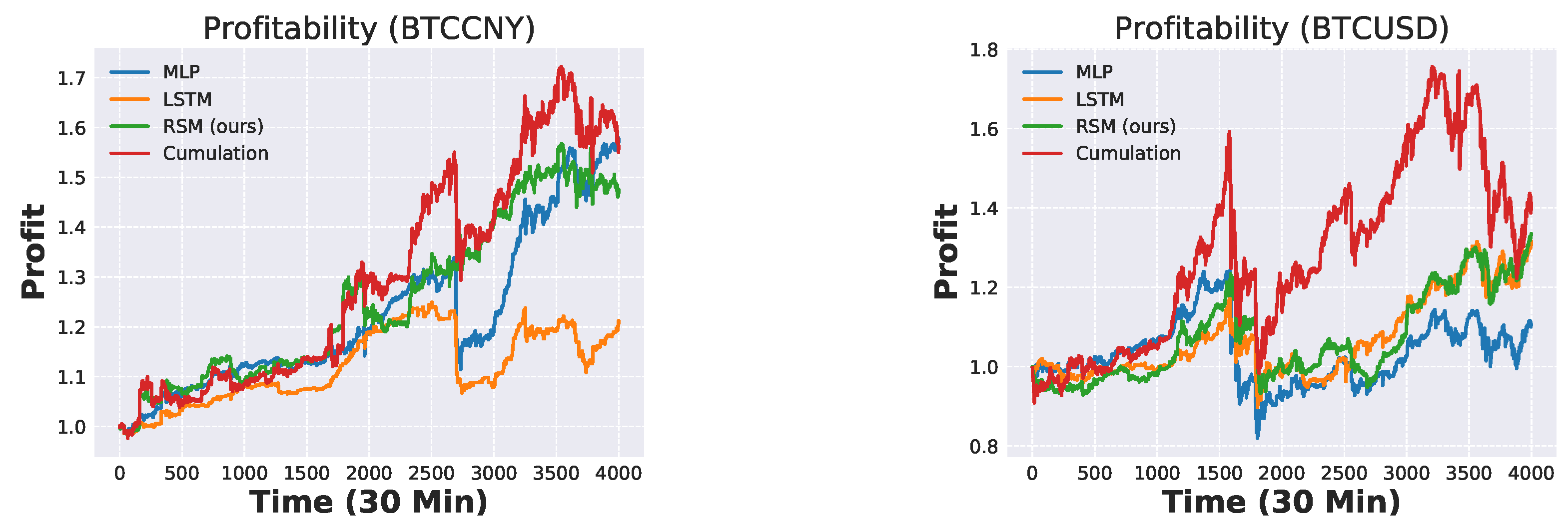
We have used multi-layer perceptron (MLP) and an LSTM network as baselines (see Appendix A for more details about LSTM). Both MLP and the LSTM network had two layers, and each layer had 32 hidden units. We computed the probability distribution and selected the class with the maximum probability. Metric scores of accuracy, recall, precision, and the F1 measure are given in Table 1 for BTCCNY dataset and in Table 2 for BTCUSD data set.
It can be seen that the three-valued classification F 1 measure increased with noise reduction and was the highest for the present model. Note that the LSTM network obtained the highest precision score because it was biased to output static. It follows that the numbers of the true positives for up and down decreased, and consequently the recall and F1 scores worsened. The reference levels for uniform class distribution in a purely-random process would be 0 . 33 3 ¯ , which were clearly exceeded by the present results by all methods. Confusion matrices for the LSTM methods and the present RSM method for both currencies, CNY and USD, are given in Figure 7 and Figure 8.

6.3. Profitability

We examine the profitability of baselines and our model, based on the prediction we obtained from the above experiment: up, down, or static for the simple moving average (the result is shown in Table 3). We define a simple trading strategy: buy Bitcoin (all funds) for prediction up; sell Bitcoin (all funds to CNY or USD) for down prediction; and no change in position (either BTC or CNY, based on the current situation) if the prediction is static. Using the present dataset sampled by minutes and the predicted classes for half-an-hour averages, we evaluated the prediction performance using a half-an-hour sampling step. The length of the testing dataset was 120k-min steps. In this setting, we used the log return defined in Equation (7) where P t is the closing price at time t and k = 30 .
R t = log P t P t k
Dynamic trading results measured on a half-an-hour trading scale are given in Figure 9. The green curve (our method) should be compared with the red curve (buy-and-hold strategy). While all strategies remained profitable in the long run, none of them outperformed the market, except for very rare intermittent periods.
It remains to be established whether a more elaborate trading scheme based on the present classification method would be able to outperform the market. An example could be using n-grams of past prediction labels, evaluating their correctness, and conditioning the next trading move based on the results. We remark here that the present success in predicting the market trend already rules out the applicability of the strong form of the efficient market hypothesis; in addition, a profitable trading strategy would rule out also its weaker form, which forbids the existence of such algorithms. Practical differences may arise for instance from the transaction fees or because of the time required to record the transactions in the blockchain (about 10 min for Bitcoin).

6.4. Alternative Sampling Schemes

We studied how changing the sampling scheme affects the performance (Table 4). We evaluated our model using the original and the alternative sampling methods. If the sampling scheme does not affect the performance, this may imply that the market dynamics does not change between the two sampling selections. To test this hypothesis, we compared sample sequences from the very first part of the dataset to classify the input sequences around the very end of the dataset, which is the essence of the alternative sampling method.
The alternative sampling thus took all samples from the first week. Interestingly, the performance of BTCUSD did not change much, whereas the performance of BTCCNY degraded dramatically. BTCCNY price at the end of 2013 went up sharply and heavily fluctuated during a few months. This degradation might be caused by this strong fluctuation, which is not observed in BTCUSD time series. The global sampling scheme used the option that all samples are taken from the whole past.

6.5. Universal Patterns

For the sake of completeness, we studied the degree of the existence of universal patterns (see (Sirignano and Cont 2018) for the formulation) empirically. We deployed the pre-trained model with fixed settings and evaluated it on the different dataset. If there were any relation among distributions of an asset on which a model was trained and another asset on which the model was tested, we could deploy the same model among different assets. The work in (Sirignano and Cont 2018) studied this type of universality extensively. Here, we used Lite Coin (LTC) in the same market as a test dataset. We used RSM, which was trained on BTCUSD (we used the same number of train data points as the experiment above) to test it on the last 120k data points of LTCCNY and LCTUSD, which were not observed in the training data. The results are shown in Table 5 and Table 6. Both the LSTM network and our model worked reasonably, and our model performed better for most information metric scores, except the precision score, for which the reason is the same as in the above section.

7. Conclusions

We proposed a new trend prediction classification learning method and showed that it performed well in the domain where taking the non-stationarity assumption was quite fair. We conducted experiments with very small scaled models to distinguish the effect of our method and confirmed its superiority in comparison with the MLP and LSTM baselines. The present method can be applied to other financial time series and is not confined to cryptocurrency markets.

Author Contributions

Conceptualization, L.P., T.S.; methodology, T.S., L.P.; software, T.S.; validation, T.S., L.P.; formal analysis, T.S., L.P.; investigation, T.S., L.P.; resources, L.P.; data curation, T.S., L.P.; writing—original draft preparation, T.S., L.P.; writing—review and editing, L.P., T.S.; visualization, T.S., L.P.; supervision, L.P.; project administration, L.P.; funding acquisition, L.P.

Funding

This research received no external funding.

Conflicts of Interest

The authors declare no conflict of interest.

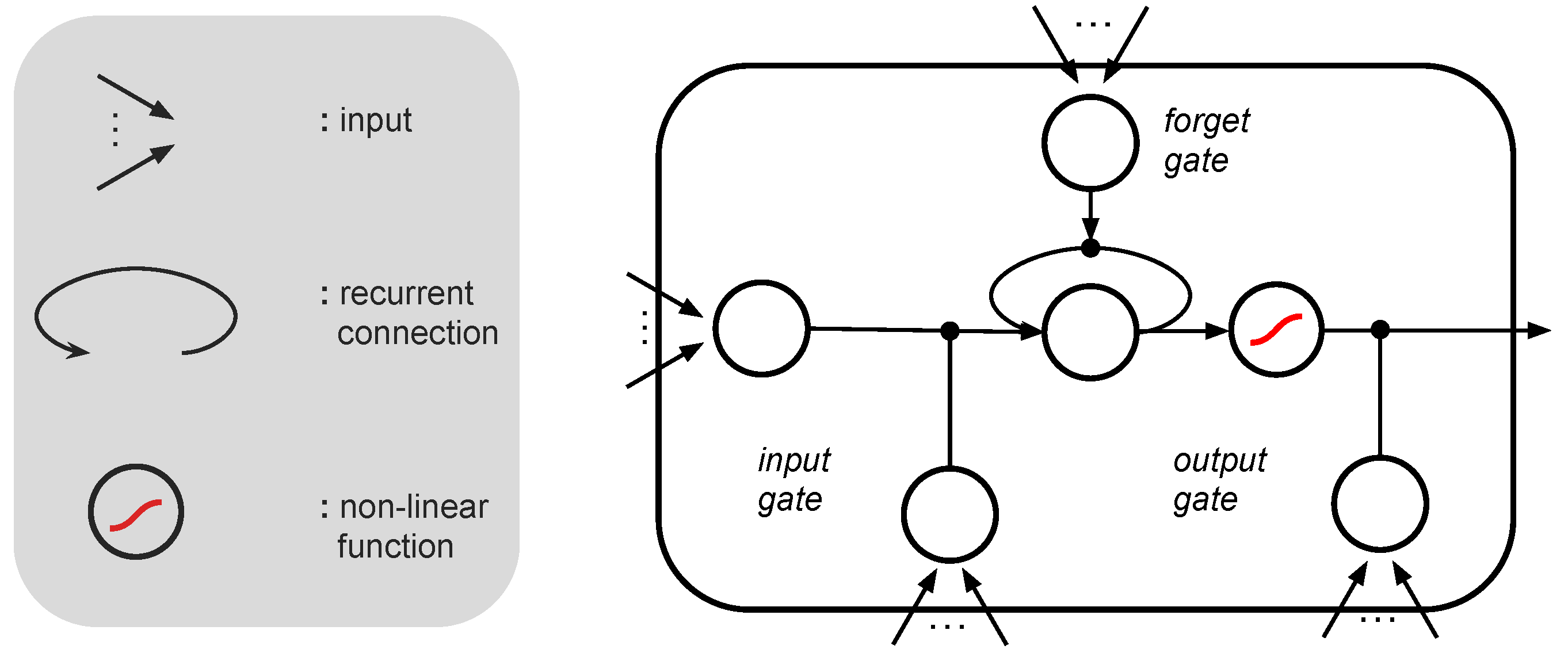
Appendix A. Long Short-Term Memory

Long short-term memory (LSTM) (Gers et al. 2000; Hochreiter and Schmidhuber 1997) is a unit for recurrent neural networks (Figure A1). LSTM deploys the gating mechanism, which is designed to solve input (output) weight conflict. It enables LSTM to capture long time dependencies and encode relatively long sequences ((Greff et al. 2017) conducted experiments on the performance of the varieties of LSTM models extensively). Because of this advantageous property, LSTM has been used in many research works (Andrychowicz et al. 2016; Bahdanau et al. 2014; Luong et al. 2015; Sutskever et al. 2014; Ravi and Larochelle 2017; Wu et al. 2016) as a core technique. Equations (A1)–(A6) are the formulation (we refer to (Greff et al. 2017)),
z t = g W z x t + R z y t 1 + b z
i t = σ W i x t + R i y t 1 + b i
f t = σ W f x t + R f y t 1 + b f
c t = z t i t + c t 1 f t
o t = σ W o x t + R o y t 1 + b o
y t = h c t o t
where W z , W i , W f , and W o are weight parameters for input, R z , R i , R f , and R o are weight parameters for recurrent input, and b z , b i , b f , and b o are biases, respectively. x t and y t 1 are input and recurrent input (note that y t 1 has a gap in time because it is a recurrent input). g , σ , and h are non-linear functions (usually, the hyperbolic tangent function is selected as g and h and the logistic sigmoid function as σ ). Capital letters in bold denote matrices, whereas lower case in bold is used for vectors. ⊙ stands for element-wise multiplication.
Figure A1. Abstract visualization of LSTM. A set of components on the left describes their roles in a unit on the right.
Jrfm 12 00017 g0a1
In Equation (A1), LSTM selectively extracts information necessary to output desired values, and the information extracted passes the input gate where LSTM determines how much information should be loaded into its memory (memory at time step t is represented as c t ) in Equation (A2). If the gate outputs one, then all the extracted information flows into its memory, and if it outputs zero, none of the extracted information is read in its memory. The forget and output gates work in the same way to adjust information flow in memory-to-memory and memory-to-output propagation segments.

References

  1. Andrychowicz, Marcin, Misha Denil, Sergio Gomez, Matthew W. Hoffman, David Pfau, Tom Schaul, Brendan Shillingford, and Nando De Freitas. 2016. Learning to learn by gradient descent by gradient descent. In Advances in Neural Information Processing Systems. Cambridge: The MIT Press, pp. 3981–89. [Google Scholar]
  2. Bahdanau, Dzmitry, Kyunghyun Cho, and Yoshua Bengio. 2014. Neural machine translation by jointly learning to align and translate. arXiv, arXiv:1409.0473. [Google Scholar]
  3. Bariviera, Aurelio F., Maria Jose Basgall, Waldo Hasperue, and Marcelo Naiouf. 2017. Some stylized facts of the bitcoin market. Physica A: Statistical Mechanics and its Applications 484: 82–90. [Google Scholar] [CrossRef]
  4. Cinbis, Ramazan Gokberk, Jakob Verbeek, and Cordelia Schmid. 2011. Unsupervised metric learning for face identification in tv video. Paper presented at the 2011 IEEE International Conference on Computer Vision (ICCV), Barcelona, Spain, November 6–13; pp. 1559–66. [Google Scholar]
  5. Dixon, Matthew, Diego Klabjan, and Jin Hoon Bang. 2017. Classification-based financial markets prediction using deep neural networks. Algorithmic Finance 6: 67–77. [Google Scholar] [CrossRef]
  6. Gers, Felix A., Jürgen Schmidhuber, and Fred A. Cummins. 2000. Learning to forget: Continual prediction with lstm. Neural Computation 12: 2451–71. [Google Scholar] [CrossRef] [PubMed]
  7. Gkillas, Konstantinos, and Paraskevi Katsiampa. 2018. An application of extreme value theory to cryptocurrencies. Economics Letters 164: 109–11. [Google Scholar] [CrossRef]
  8. Gkillas, Konstantinos, Stelios Bekiros, and Costas Siriopoulos. 2018. Extreme Correlation in Cryptocurrency Markets. Available online: https://ssrn.com/abstract=3180934 (accessed on 14 January 2019).
  9. Glorot, Xavier, Antoine Bordes, and Yoshua Bengio. 2011. Deep sparse rectifier neural networks. In Paper presented at the Proceedings of the Fourteenth International Conference on Artificial Intelligence and Statistics, Ft. Lauderdale, FL, USA, April 11–13; pp. 315–23. [Google Scholar]
  10. Graves, Alex, Greg Wayne, and Ivo Danihelka. 2014. Neural turing machines. arXiv, arXiv:1410.5401. [Google Scholar]
  11. Greff, Klaus, Rupesh K. Srivastava, Jan Koutník, Bas R. Steunebrink, and Jürgen Schmidhuber. 2017. Lstm: A search space odyssey. IEEE Transactions on Neural Networks and Learning Systems 28: 2222–32. [Google Scholar] [CrossRef] [PubMed]
  12. Hilliard, Nathan, Lawrence Phillips, Scott Howland, Artem Yankov, Courtney D. Corley, and Nathan O. Hodas. 2018. Few-shot learning with metric-agnostic conditional embeddings. arXiv, arXiv:1802.04376. [Google Scholar]
  13. Hochreiter, Sepp, and Jürgen Schmidhuber. 1997. Long short-term memory. Neural Computation 9: 1735–80. [Google Scholar] [CrossRef] [PubMed]
  14. Kingma, Diederik P., and Jimmy Ba. 2014. Adam: A method for stochastic optimization. arXiv, arXiv:1412.6980. [Google Scholar]
  15. Koch, Gregory. 2015. Siamese neural networks for one-shot image recognition. Paper presented at the 32 nd International Conference on Machine Learning, Lille, France, July 6–11. [Google Scholar]
  16. Koutmos, Dimitrios. 2018. Bitcoin returns and transaction activity. Economics Letters 167: 81–85. [Google Scholar] [CrossRef]
  17. Kristoufek, Ladislav. 2018. On bitcoin markets (in)efficiency and its evolution. Physica A: Statistical Mechanics and its Applications 503: 257–62. [Google Scholar] [CrossRef]
  18. Lake, Brenden, Chia-ying Lee, James Glass, and Josh Tenenbaum. 2014. One-shot learning of generative speech concepts. Paper presented at Annual Meeting of the Cognitive Science Society, Quebec City, QC, Canada, July 23–26; vol. 36. [Google Scholar]
  19. Lake, Brenden, Ruslan Salakhutdinov, Jason Gross, and Joshua Tenenbaum. 2011. One shot learning of simple visual concepts. Paper presented at Annual Meeting of the Cognitive Science Society, Boston, MA, USA, July 20–23; vol. 33. [Google Scholar]
  20. Lake, Brenden M., Ruslan Salakhutdinov, and Joshua B. Tenenbaum. 2015. Human-level concept learning through probabilistic program induction. Science 350: 1332–38. [Google Scholar] [CrossRef] [PubMed]
  21. Li, Fe-Fei, Rob Fergus, and Pietro Perona. 2003. A bayesian approach to unsupervised one-shot learning of object categories. Paper presented at the 2003 Ninth IEEE International Conference on Computer Vision, Nice, France, October 13–16; pp. 1134–41. [Google Scholar]
  22. Li, Fei-Fei, Rob Fergus, and Pietro Perona. 2006. One-shot learning of object categories. IEEE Transactions on Pattern Analysis and Machine Intelligence 28: 594–611. [Google Scholar] [Green Version]
  23. Luong, Minh-Thang, Hieu Pham, and Christopher D. Manning. 2015. Effective approaches to attention-based neural machine translation. arXiv, arXiv:1508.04025. [Google Scholar]
  24. Mäkinen, Milla, Juho Kanniainen, Moncef Gabbouj, and Alexandros Iosifidis. 2018. Forecasting of jump arrivals in stock prices: New attention-based network architecture using limit order book data. arXiv, arXiv:1810.10845. [Google Scholar]
  25. Ravi, Sachin, and Hugo Larochelle. 2017. Optimization as a model for few-shot learning. Paper presented at International Conference on Learning Representations (ICLR), Toulon, France, April 24–26. [Google Scholar]
  26. Santoro, Adam, Sergey Bartunov, Matthew Botvinick, Daan Wierstra, and Timothy Lillicrap. 2016. One-shot learning with memory-augmented neural networks. arXiv, arXiv:1605.06065. [Google Scholar]
  27. Schuster, Mike, and Kuldip K Paliwal. 1997. Bidirectional recurrent neural networks. IEEE Transactions on Signal Processing 45: 2673–81. [Google Scholar] [CrossRef]
  28. Sirignano, Justin, and Rama Cont. 2018. Universal Features of Price Formation in Financial Markets: Perspectives From Deep Learning. Available online: https://ssrn.com/abstract=3141294 (accessed on 1 December 2018).[Green Version]
  29. Sutskever, Ilya, Oriol Vinyals, and Quoc V. Le. 2014. Sequence to sequence learning with neural networks. In Advances in Neural Information Processing Systems. Cambridge: The MIT Press, pp. 3104–12. [Google Scholar]
  30. Vinyals, Oriol, Charles Blundell, Timothy Lillicrap, Koray Kavukcuoglu, and Daan Wierstra. 2016. Matching networks for one shot learning. In Advances in Neural Information Processing Systems. Cambridge: The MIT Press, pp. 3630–38. [Google Scholar]
  31. Wu, Yonghui, Mike Schuster, Zhifeng Chen, Quoc V. Le, Mohammad Norouzi, Wolfgang Macherey, Maxim Krikun, Yuan Cao, Qin Gao, Klaus Macherey, and et al. 2016. Google’s neural machine translation system: Bridging the gap between human and machine translation. arXiv, arXiv:1609.08144. [Google Scholar]
  32. Xing, Eric P., Michael I. Jordan, Stuart J. Russell, and Andrew Y. Ng. 2003. Distance metric learning with application to clustering with side-information. In Advances in Neural Information Processing Systems. Cambridge: The MIT Press, pp. 521–28. [Google Scholar]
  33. Yao, Yushi, and Zheng Huang. 2016. Bi-directional LSTM recurrent neural network for chinese word segmentation. arXiv, arXiv:1602.04874. [Google Scholar]
  34. Zhang, Zihao, Stefan Zohren, and Stephen Roberts. 2018. Deeplob: Deep convolutional neural networks for limit order books. arXiv, arXiv:1808.03668. [Google Scholar]
Figure 1. Visualization for walk-forward optimization. It uses the data points in a train window (green box) and a test window (red box), one at a time. After finishing training a model with the dataset, the two windows move to the right, and training begins again until the windows hit the end of the time series.
Jrfm 12 00017 g001
Figure 2. Visualization of the pipeline. Given inputs x t ( i n p u t ) , sequences x t ( u p ) , x t ( d o w n ) , x t ( s t a t i c ) are randomly sampled in the red window. Then, the input and samples are independently encoded with LSTMNet (Equation (3)) and bi-directional LSTMNet (Equation (4)). Refer to the text for more details.
Jrfm 12 00017 g002
Figure 3. OHLC plot (Bitcoin price in CNY). The price peaks at the end of 2013 and gradually decreases toward the middle of 2015. Then, it recovers and peaks at the beginning of 2017. The price forms a u-shape in the long run. Note that the price highly fluctuates at the beginning of 2017 when Bitcoin markets were regulated in China. This caused class imbalance in the testing dataset (Figure 6).
Jrfm 12 00017 g003
Figure 4. OHLC plot (Bitcoin price in USD). The dataset begins at the latter half of 2014. The price peaks at the beginning of 2017 in the same way as CNY, cf. Figure 3. Transaction volume was relatively constant before June 2016, whereas the volume of BTCCNY transactions in Figure 3 increased dramatically after the beginning of 2016.
Jrfm 12 00017 g004
Figure 5. Distribution of high-frequency returns computed from closing prices on a minute scale and a half-an-hour scale for Bitcoin prices in CNY (black) and USD (red). A non-Gaussian shape is observed in all cases.
Jrfm 12 00017 g005
Figure 6. Comparative histogram of training and testing data points (BTCCNY in the OkCoin market). It shows that there was a crucial class imbalance in the testing data, whereas the data points in the training data were relatively balanced. This imbalance is also implied in Figure 3.
Jrfm 12 00017 g006
Figure 7. Confusion matrices (LSTM). The x-axis is the prediction, and the y-axis is the true label. Matrices at the top are unnormalized, and the ones at the bottom are normalized. Both unnormalized and normalized matrices are given because there was a crucial class imbalance (Figure 6). As compared to the matrices of Figure 8, the ratio of static prediction became higher.
Jrfm 12 00017 g007
Figure 8. Confusion matrices (RSM). Refer to Figure 7 for the axis labels. As compared to the confusion matrices of an LSTM network, it can be seen that our model was less biased to the static class.
Jrfm 12 00017 g008
Figure 9. Visualization for profitability of BTCCNY (left) and BTCUSD (right) at each time step. Cumulation on each graph denotes the exponential of the cumulative log return value at that time step. Refer to Figure 3 and Figure 4 for price.
Jrfm 12 00017 g009
Table 1. Model evaluation scores on accuracy, recall, precision, and F1 measure. Bitcoin price in Chinese yuan (BTCCNY) from the OkCoin market is used as the dataset. We use the last 120k data points for the evaluation, which were not used in training and validation. RSM, random sampling method. The highest score among the methods is printed in bold in each column.
AccuracyRecallPrecisionF1 Score
MLP0.47660.45700.48220.4511
LSTM0.46880.48770.55810.4657
RSM (ours)0.53530.51820.54580.5092
Table 2. Model evaluation scores on accuracy, recall, precision, and F1 measure. Bitcoin price in U.S. dollar (BTCUSD) from the OkCoin market was used as the dataset. We used the last 120k data points for the evaluation, which were not used in training and validation.
AccuracyRecallPrecisionF1 Score
MLP0.55590.49450.49780.4786
LSTM0.57590.54640.57170.5034
RSM (ours)0.62640.55380.54880.5367
Table 3. The profitability factor of BTCCNY and BTCUSD in the OkCoin market. BTCCNY and BTCUSD prices showed two bubble bursts (Figure 3 and Figure 4). The values are exponentials of the log return accumulated from trades. Market reference values were 1.5643 for BTCCNY and 1.4122 for BTCUSD (a value of 1 represents 100% of the initial investment). Refer to the text for details.
CNYUSD
MLP1.57871.1055
LSTM1.21241.3157
RSM (ours)1.47611.3346
Table 4. Model evaluation scores on BTCCNY. We deployed 2 different sampling schemes. Refer to the text for details.
AccuracyRecallPrecisionF1 Score
first week0.40310.48600.60760.4152
global0.53640.52380.55030.5124
Table 5. Universal patterns (LTCCNY). Model evaluation scores use the same metric as in Table 1. We evaluated the same baselines and our model on a different dataset from the dataset on which they were trained. Lite Coin Chinese yuan (LTCCNY) in the OkCoin market was used as the evaluation dataset. We used the parameters optimized on BTCUSD.
AccuracyRecallPrecisionF1 Score
MLP0.49920.50040.51760.5005
LSTM0.54750.54520.56680.5492
RSM (ours)0.57460.56950.57620.5713
Table 6. Universal patterns (LTCUSD). Model evaluation scores use the same metric as in Table 1. We evaluated the same baselines and our model on a different dataset from the dataset on which they were trained. Lite Coin US dollar (LTCUSD) in the OkCoin market was used as the evaluation dataset. We used the parameters optimized on  BTCUSD.
AccuracyRecallPrecisionF1 Score
MLP0.49170.49270.50520.4905
LSTM0.52420.53320.57520.5291
RSM (ours)0.55260.55040.56370.5499

