Does the Assumption on Innovation Process Play an Important Role for Filtered Historical Simulation Model?

Abstract

Most of the financial institutions compute the Value-at-Risk (VaR) of their trading portfolios using historical simulation-based methods. In this paper, we examine the Filtered Historical Simulation (FHS) model introduced by Barone-Adesi et al. (1999) theoretically and empirically. The main goal of this study is to find an answer for the following question: “Does the assumption on innovation process play an important role for the Filtered Historical Simulation model?”. For this goal, we investigate the performance of FHS model with skewed and fat-tailed innovations distributions such as normal, skew normal, Student’s-t, skew-T, generalized error, and skewed generalized error distributions. The performances of FHS models are evaluated by means of unconditional and conditional likelihood ratio tests and loss functions. Based on the empirical results, we conclude that the FHS models with generalized error and skew-T distributions produce more accurate VaR forecasts.

1. Introduction

The most well known risk measure, Value-at-Risk (VaR), is used to measure and quantify the level of financial risk within a firm or investment portfolio over a specific holding period. The VaR measures the potential loss of risky asset or portfolio over a defined period and for a given confidence level. The VaR is defined as

$$Va{R}_p=F^{-1}(1-p),$$

(1)

where F is the cumulative distribution function (cdf) of financial losses, $F^{-1}$ denotes the inverse of F and p is the quantile at which VaR is calculated. The approaches to VaR could be investigated in three categories: (i) fully parametric models approach based on a volatility models; (ii) non-parametric approaches based on the Historical Simulation (HS) methods and (iii) Extreme Value Theory approach based on modeling the tails of the return distribution.

In this paper, we focus on the non-parametric HS models. The HS model is based on the assumption that historical distribution of returns will remain the same over the next periods. The HS model assumes that price change behaviour repeats itself over the time. Thus, future distribution of asset returns could be described by the empirical one. The one-day-ahead VaR R forecast for HS model is given by

$$Va{R}_{t+1}=Quantile\left\{{\left\{X_t\right\}}_{t=1}^n,p\right\},$$

(2)

where p is the quantile at which VaR is calculated. Mögel and Auer (2017) compared the performance of HS model with several competitive VaR models and stated that HS model produces the similar VaR forecasts with unconditional generalized Pareto distribution.

The HS model has several advantages. For instance, it is easy to understand and implement. It is a nonparametric model and does not require any distributional assumption. However, the HS model has also several shortcomings. The HS model ignores the time-varying volatility dynamics. In order to remove lack of HS model, Hull and White (1998) and Barone-Adesi et al. (1999) introduced the FHS model. This approach can be viewed as mixture of the HS and the Generalized Autoregressive Conditional Heteroskedasticity (GARCH) models. Specifically, it does not make any distributional assumption about the standardized returns, while it forecasts the variance through a volatility model. Hence, it is mixture of parametric and non-parametric statistical procedures. Barone-Adesi and Giannopoulos (2001) demonstrated the usefulness of the FHS model over the historical one. Kuester et al. (2006) compared the forecasting performance of several advanced VaR models. Kuester et al. (2006) concluded that GARCH-Skew-T, Extreme Value Theory (EVT) approach with normal and Skew-T innovations and FHS model with normal and Skew-T innovations perform the best. Angelidis et al. (2007) compared the FHS model with GARCH models specified under different innovation distributions such as normal, Student’s-t and Skewed-T. Roy (2011) estimated the VaR of the daily return of Indian capital market using FHS model. Omari (2017) compared FHS, Exponentially Weighted Moving Average (EWMA), GARCH-normal, GARCH-Student’s-t, GJR-GARCH-normal and GJR-GARCH-Student’s-t models in terms of accuracy of VAR forecasts. Omari (2017) demonstrated that GJR-GARCH-Stundet’s-t approach and Filtered Historical Simulation method with GARCH volatility specification perform competitively accurate in estimating VaR forecasts for both standard and more extreme quantiles thereby generally out-performing all the other models under consideration.

The goal of this paper is to investigate the VaR forecasting performance of the FHS model specified under skewed and fat-tailed innovations distributions. For this goal, the comprehensive introduction to the FHS and GARCH models is given. The FHS model under six innovation distributions are introduced. Rolling window estimation produce is used to obtain both unknown parameters of GARCH models and VaR forecasts. The performance of the FHS models, in terms of accuracy of VaR forecasts, are evaluated by means of backtesting methods and loss functions.

The rest of the paper is organized as follows: Section 2 is devoted to theoretical properties of the FHS and GARCH models under normal, Student’s-t, skew-normal, skew-T, generalized error and skewed generalized error innovation distributions. Backtesting methodology is given in Section 3. Empirical findings and model comparisons are presented in Section 4. Concluding remarks are given in Section 5.

2. Filtered Historical Simulation Models

In this section, the FHS model is defined. Then, the log-likelihood functions of GARCH model specified under normal, skew-normal, Student’s-t, skew-T, generalized error and skewed genealized error innovation distributions are presented.

FHS model can be summarized as follows:

√

Let $R_t$ denotes the daily log-returns. The benchmark GARCH(1,1) model, introduced by Bollerslev (1986), is defined by

$$\begin{array}{c}{R}_t=\mu +e_t,\hfill \\ e_t={\epsilon }_t{h}_t,{\epsilon }_t\sim i.i.d.\hfill \\ h_t^2=\omega +{\gamma }_1{e}_{t-1}^2+{\gamma }_2{h}_{t-1}^2,\hfill \end{array}$$

(3)

where $\omega >0$, ${\gamma }_1>0$,${\gamma }_2>0$, ${\mu }_t$ and $h_t^2$ are the conditional mean and variance, respectively, and ${\epsilon }_t$ is the innovation distribution with zero mean and unit variance. Maximum Likelihood Estimation (MLE) method is widely used to estimate parameters of GARCH models. Under the assumption of independently and identically distributed (iid) innovations with $f\left({\epsilon }_t;\tau \right)$ density function, the log-likelihood function of $r_t$ for a sample of T observations is given by

$$\ell \left(\psi \right)={\displaystyle \sum _{t=1}^T}\left[\ln \left(f\left({\epsilon }_t;\tau \right)\right)-\frac{1}{2}\ln \left(h_t^2\right)\right]$$

(4)

where $\psi =\left(\mu ,\omega ,{\gamma }_1,{\gamma }_2,\tau \right)$ is the parameter vector of GARCH model, $\tau$ is the shape parameter(s) of $f\left({\epsilon }_t;\tau \right)$ and ${\epsilon }_t=\frac{e_t}{h_t}$.

The standardized residuals of estimated GARCH(1,1) model are extracted as follows:

$${\epsilon }_t=\frac{{\widehat{e}}_t}{{\widehat{h}}_t},$$

(5)

where ${\widehat{e}}_t$ is the estimated residual and ${\widehat{h}}_t$ is the corresponding daily estimated volatility.

Now, we can generate the first simulated residual by randomly (with replacement) draw standardized residuals from the dataset with multiplying the one-day ahead volatility forecast:

$$z_{t+1}^{\ast }=e_1^{\ast }{h}_{t+1}.$$

(6)

The first simulated return for period $t+1$ can be obtained as follows:

$$R_{t+1}^{\ast }={\mu }_{t+1}+z_{t+1}^{\ast },$$

(7)

where $z_{t+1}^{\ast }$ is the first simulated residual for period $t+1$.

This procedure is repeated B times of length T. Here, B represents the number of bootstrapped samples and T represents the each of bootstrapped sample size. Then, VaR for period $t+1$ can be forecasted as follows:

$$Va{R}_{t+1}=\frac{{\displaystyle \sum _{b=1}^B}Quantile\left\{{\left\{R_t^{\ast }\right\}}_{t=1}^T, 100p\right\}}{B}.$$

(8)

The rest of this section is devoted to present the log-likelihood functions of GARCH model under normal, skew-normal, Student’s-t, skew-T, generalized error and skewed generalized error distributions.

2.1. Normal Distribution

The log-likelihood function of the GARCH model specified under normal innovations is given by

$$\ell (\psi )=-0.5\left(T \ln 2\pi +{\displaystyle \sum _{t=1}^T}\ln h_t^2+{\displaystyle \sum _{t=1}^T}{\epsilon }_t^2\right),$$

(9)

where $\psi =(\mu ,\omega ,{\gamma }_1,{\gamma }_2)$ denotes the parameter vector of the GARCH-normal (GARCH-N) model and $h_t^2=\omega +{\gamma }_1{e}_{t-1}^2+{\gamma }_2{h}_{t-1}^2$.

2.2. Skew-Normal Distribution

The first skew extension of normal distribution was proposed by Azzalini (1985). The probability density function (pdf) of skew-normal (SN) distribution is given by

$$\varphi \left(z;\lambda \right)=2\varphi \left(z\right)\Phi \left(z\lambda \right),\mathrm{z}\in \Re , \lambda \in \Re ,$$

(10)

where $\lambda$ is an additional parameter that controls the skewness. When $\lambda <0$, the SN distribution is left skewed, otherwise, it is right skewed. If $\lambda =0$, the SN distribution reduces to standard normal distribution. The kth moment of SN distribution is given by

$$E\left(Z^{2k+1}\right)=\sqrt{\frac{2}{\pi }}\frac{\left(2k+1\right)!}{2^{k}k!}{\displaystyle \sum _{i=0}^k}{\left(-1\right)}^i\left(\begin{array}{c}k\hfill \\ i\hfill \end{array}\right)\frac{{\delta }^{2i+1}}{2i+1}.$$

(11)

here, $k=0,1,2,\dots ,n$ and $\delta =\lambda /\phantom{\lambda \sqrt{1+{\lambda }^2}}\sqrt{1+{\lambda }^2}$. Note that the even moments of the SN distribution are equal to standard normal distribution. The mean and variance of SN distribution is, respectively, given by,

$$\begin{array}{c}\mu =b\delta \hfill \\ {\sigma }^2=1-{\left(b\delta \right)}^2\hfill \end{array}$$

(12)

where $b=\sqrt{\frac{2}{\pi }}$. The standardized SN distribution is obtained using the transformed random variable $\epsilon =\left(z-\mu \right)/\phantom{\left(z-\mu \right)\sigma }\sigma$ where $E\left(\epsilon \right)=0$ and $\mathrm{var}\left(\epsilon \right)=1$. The random variable z can be expressed as $z=\epsilon \sigma +\mu$ and $\partial z/\phantom{\partial z\partial \epsilon }\partial \epsilon =\sigma$. Thus, the pdf of the standardized SN distribution is given by

$$f\left(\epsilon ;\lambda \right)=2\sigma \varphi \left((\epsilon \sigma +\mu )\right)\Phi \left((\epsilon \sigma +\mu )\lambda \right)$$

(13)

Hereafter, using the standardized SN distribution, the log-likelihood function of GARCH model with SN innovation distribution is given by

$$\ell \left(\psi \right)={\displaystyle \sum _{t=1}^T}\ln \left[2\sigma \varphi \left({\epsilon }_t\sigma +\mu \right)\right]+{\displaystyle \sum _{t=1}^T}\ln \left[\Phi \left(\left({\epsilon }_t\sigma +\mu \right)\lambda \right)\right]-\frac{1}{2}{\displaystyle \sum _{t=1}^T}\ln \left(h_t^2\right),$$

(14)

where $\psi =\left(\mu ,\omega ,{\gamma }_1,{\gamma }_2,\lambda \right)$ is the parameter vector.

2.3. Student’s-t Distribution

Since financial return series has fatter tails than normal distribution, Bollerslev (1986, 1987) proposed the GARCH model with the Student’s-t innovations. GARCH model with the Student’s-t innovations enables to model both fat-tail and excess kurtosis observed in financial return series. The log-likelihood function of the GARCH-Student’s-t (GARCH-T) model is given by

$$\begin{array}{c}\ell (\psi )=T\left[\ln \Gamma \left(\frac{\upsilon +1}{2}\right)-\ln \Gamma \left(\frac{\upsilon }{2}\right)-\frac{1}{2}\ln \left[\pi (\upsilon -2)\right]\right]\hfill \\ -\frac{1}{2}{\displaystyle \sum _{t=1}^T}\left[\ln h_t^2+\left(1+\upsilon \right)\ln \left(1+\frac{{\epsilon }_t^2}{\upsilon -2}\right)\right]\hfill \end{array},$$

(15)

where $\psi =(\mu ,\omega ,{\gamma }_1,{\gamma }_2,\upsilon )$ is the parameter vector, $\Gamma (\upsilon )$ is the gamma function and parameter $\upsilon$ controls the tails of the distribution.

2.4. Skew-T Distribution

The pdf of skew-T distribution obtained by Azzalini and Capitanio (2003) is given by

$$f\left(x;\lambda ,\upsilon \right)=2t\left(x;\upsilon \right)T\left(\sqrt{\frac{1+\upsilon }{x^2+\upsilon }}\lambda t;\upsilon +1\right), x\in \Re ,$$

(16)

where $t\left(·\right)$ and $T\left(·\right)$ are pdf and cdf of Student’s-t distribution, respectively, and $\lambda$ controls the skewness. When $\lambda =0$, ST distribution reduces to Student’s-t distribution in Equation (16). The moments of ST distribution are given by

$$E\left(X^k\right)=\frac{{\left(\frac{\upsilon }{2}\right)}^{\frac{k}{2}}\Gamma \left(\frac{\left(\upsilon -k\right)}{2}\right)}{\Gamma \left(\frac{\upsilon }{2}\right)}E\left(Z^k\right),$$

(17)

The mean and variance of ST distribution are, respectively, given by

$$\begin{array}{c}\mu =\frac{{\left(\frac{\upsilon }{\pi }\right)}^{\frac{1}{2}}\Gamma \left(\frac{\left(\upsilon -1\right)}{2}\right)}{\Gamma \left(\frac{\upsilon }{2}\right)}\frac{\lambda }{\sqrt{1+{\lambda }^2}}\hfill \\ ,{\sigma }^2=\left(\frac{\upsilon }{\upsilon -2}-{\mu }^2\right).\hfill \end{array}$$

(18)

The standardized ST distribution is obtained using the transformed random variable $\epsilon =\left(z-\mu \right)/\phantom{\left(z-\mu \right)\sigma }\sigma$, where $E\left(\epsilon \right)=0$ and $\mathrm{var}\left(\epsilon \right)=1$. The random variable z can be expressed as $z=\epsilon \sigma +\mu$ and $\partial z/\phantom{\partial z\partial \epsilon }\partial \epsilon =\sigma$. Thus, the pdf of standardized ST distribution is given by

$$f\left(\epsilon ;\lambda ,\upsilon \right)=2\sigma t\left(\left(\epsilon \sigma +\mu \right);\upsilon \right)T\left(\sqrt{\frac{1+\upsilon }{{\left(\epsilon \sigma +\mu \right)}^2+\upsilon }}\lambda \left(\epsilon \sigma +\mu \right);\upsilon +1\right), \upsilon >2$$

(19)

where $\mu$ and $\sigma$ are mean and standard deviation of ST distribution, respectively. The log-likelihood function of GARCH model with the ST innovation distribution is given by

$$\begin{array}{c}\ell \left(\psi \right)=T \ln \left(2\right)+T \ln \left(\sigma \right)+{\displaystyle \sum _{t=1}^T}\ln \left[t\left(\left({\epsilon }_t\sigma +\mu \right);\upsilon \right)\right]\hfill \\ +{\displaystyle \sum _{t=1}^T}\ln \left[T\left(\sqrt{\frac{1+\upsilon }{{\left({\epsilon }_t\sigma +\mu \right)}^2+\upsilon }}\lambda \left({\epsilon }_t\sigma +\mu \right);\upsilon +1\right)\right]-\frac{1}{2}{\displaystyle \sum _{t=1}^T}\ln \left(h_t^2\right)\hfill \end{array}$$

(20)

where $\psi =\left(\mu ,\omega ,{\gamma }_1,{\gamma }_2,\lambda ,\upsilon \right)$ is the parameter vector.

2.5. Generalized Error Distribution

Nelson (1991) introduced the GARCH volatility model of generalized error distribution (GED). The log-likelihood function of GARCH-GED model is given by

$$\ell (\psi )={\displaystyle \sum _{t=1}^T}\left[\ln \left(\frac{\upsilon }{2}\right)-\frac{1}{2}{\left|\frac{{\epsilon }_t}{\lambda }\right|}^{\upsilon }-(1+{\upsilon }^{-1})\ln (2)-\ln \Gamma \left(\frac{1}{2}\right)-\frac{1}{2}\ln \left(h_t^2\right)\right]$$

(21)

where $\psi =\left(\mu ,\omega ,{\gamma }_1,{\gamma }_2,\upsilon \right)$ is the parameter vector, $\upsilon$ is tail-thickness parameter and

$$\lambda ={\left(\frac{\Gamma \left(\frac{1}{\upsilon }\right)}{2^{\frac{2}{\upsilon }}\Gamma \left(\frac{3}{\upsilon }\right)}\right)}^{\frac{1}{2}}.$$

(22)

Note that the normal distribution is a special case of the GED when $\upsilon =2$. If $\upsilon <2$, the GED has heavier tails than the Gaussian distribution.

2.6. Skewed Generalized Error Distribution

Skewed Generalized Error Distribution (SGED) provides an opportunity to model skewness and excess kurtosis observed in financial return series. Lee et al. (2008) introduced the GARCH-SGED model and concluded that GARCH model with SGED innovation process outperformed the GARCH-N model for all confidence levels.

The pdf of standardized SGED is given by,

$$f({\epsilon }_t)=C\exp \left(-\frac{{\left|{\epsilon }_t+\delta \right|}^{\kappa }}{{\left[1+sign({\epsilon }_t+\delta )\lambda \right]}^{\kappa }{\theta }^{\kappa }}\right)$$

(23)

where

$$\begin{array}{c}C=\frac{\kappa }{2\theta }\Gamma {\left(\frac{1}{\kappa }\right)}^{-1},\theta =\Gamma {\left(\frac{1}{\kappa }\right)}^{0.5}\Gamma {\left(\frac{3}{\kappa }\right)}^{0.5}S{(\lambda )}^{-1}\hfill \\ S(\lambda )=\sqrt{1+3{\lambda }^2-4A^2{\lambda }^2},\delta =\frac{2\lambda A}{S(\lambda )}\hfill \\ A=\Gamma \left(\frac{2}{\kappa }\right)\Gamma {\left(\frac{1}{\kappa }\right)}^{-0.5}\Gamma {\left(\frac{3}{\kappa }\right)}^{-0.5},\hfill \end{array}$$

(24)

where $\kappa >0$ is the shape parameter, $-1<\lambda <1$ is skewness parameter. The SGED turns out to be the standard normal distribution when $\kappa =2$ and $\lambda =0$. The log-likelihood function of GARCH-SGED model is given by

$$\ell (\psi )=-{\displaystyle \sum _{t=1}^T}\left(\frac{{\left|{\epsilon }_t+\delta \right|}^{\kappa }}{{\left[1+sign\left({\epsilon }_t+\delta \right)\lambda \right]}^{\kappa }{\theta }^{\kappa }}\right)+T \ln \left(c\right)-{\displaystyle \sum _{t=1}^T}\ln \left(h_t\right)$$

(25)

where $\psi =\left(\mu ,\omega ,{\gamma }_1,{\gamma }_2,\lambda ,\kappa \right)$ is the parameter vector.

3. Evaluation of VaR Forecasts

Now, we introduce backtesting methodology that is used to compare VaR forecast accuracy of the models. Statistical accuracy of the models is evaluated by backtests of Kupiec (1995), Christoffersen (1998), Engle and Manganelli (2004) and Sarma et al. (2003). Recently, some alternative backtesting methods for VaR forecasts were proposed by Ziggel et al. (2014) and Dumitrescu et al. (2012).

Kupiec (1995) proposed a likelihood ratio (LR) test of unconditional coverage ($L{R}_{uc}$) to evaluate the model accuracy. The test examines whether the failure rate is equal to the expected value. The LR test statistic is given by

$$LR=-2\ln \left[\frac{p^{n_1}{(1-p)}^{n_0}}{{\widehat{\pi }}^{n_1}{(1-\pi )}^{n_0}}\right]\sim {\chi }_1^2,$$

(26)

where $\widehat{\pi }=n_1/(n_0+n_1)$ is the MLE of p, $n_1$ represents the total violation and $n_0$ represents the total non-violations forecasts. Violation means that if $Va{R}_t>r_t$, violation occurs, opposite case indicates the non-violation. Under the null hypothesis $(H_0:p=\widehat{\pi })$, the LR statistic follows a chi-square distribution with one degree of freedom.

The $L{R}_{uc}$ test fails to detect if violations are not randomly distributed. Christoffersen (1998) proposed a LR test of conditional coverage $L{R}_{cc}$ to remove the lack of Kupiec (1995) test. The $L{R}_{cc}$ test investigates both equality of failure rate and expected one and also independently distributed violations. The $L{R}_{cc}$ test statistic under the null hypothesis shows that the failures are independent and equal to the expected one. It is given by

$$L{R}_{cc}=-2\ln \left[\frac{{\left(1-\alpha \right)}^{n_0}{\alpha }^{n_1}}{{\left(1-{\pi }_{01}\right)}^{n_{00}}{{\pi }_{01}}^{n_{01}}{\left(1-{\pi }_{11}\right)}^{n_{10}}{{\pi }_{11}}^{n_{11}}}\right]\sim {\chi }_2^2,$$

(27)

where $n_{ij}$ is the number of observations with value i followed by j for $i,j=0,1$ and ${\pi }_{ij}=n_{ij}/{\displaystyle \sum _j}{n}_{ij}$ is the probability, for $i,j=1$. It denotes that the violation occurred, otherwise indicates the opposite case. The $L{R}_{cc}$ statistic follows a chi-square distribution with two degrees of freedom.

The Dynamic Quantile (DQ) test, proposed by Engle and Manganelli (2004), examines if the violations is uncorrelated with any variable that belongs to information set ${\Omega }_{t+1}$ when the VaR is calculated. The main idea of DQ test is to regress the current violations on past violations in order to test for different restrictions on the parameters of the model. The estimated linear regression model is given by

$$I_t={\beta }_0+{\displaystyle \sum _{i=1}^p}{\beta }_i{I}_{t-i}+{\displaystyle \sum _{i=1}^q}{\mu }_j{X}_j+{\epsilon }_t$$

(28)

where

$$I_t=\left\{\begin{array}{c}1, {\mathrm{r}}_{\mathrm{t}}<\mathrm{Va}{\mathrm{R}}_{\mathrm{t}}\hfill \\ 0, {\mathrm{r}}_{\mathrm{t}}\ge \mathrm{Va}{\mathrm{R}}_{\mathrm{t}}\hfill \end{array}\right.$$

(29)

This regression model tests whether the probability of violation depends on the level of the VaR. Here, p and q are used as 5 and 1, respectively, for illustrative purpose.

In most instances, evaluating the performance of VaR models by means of $L{R}_{uc}$, $L{R}_{cc}$ and $DC$ tests may not be sufficient to decide the most adequate model among others. For instance, some models may have the same violation number with different forecast errors. Sarma et al. (2003) defined a test on the basis of regulator’s loss function (RLF) to take into account differences between realized returns and VaR forecasts. The RLF is given by

$$RL{F}_{t+1}=\left\{\begin{array}{ccc}{\left(r_{t+1}-Va{R}_{t+1}\right)}^2,\hfill & \mathrm{if}\hfill & r_{t+1}<Va{R}_{t+1}\hfill \\ 0,\hfill & \mathrm{if}\hfill & r_{t+1}\ge Va{R}_{t+1}\hfill \end{array}\right.$$

(30)

where $Va{R}_{t+1}$ represents the one-day-ahead VaR forecast for a long position.

The unexpected loss (UL) is equal to average value of differences between realized return and VaR forecasts. The one-day-ahead magnitude of the violation for long position is given by

$${\mathrm{UL}}_{t+1}=\left\{\begin{array}{ccc}\left(r_{t+1}-Va{R}_{t+1}\right)\hfill & \mathrm{if}\hfill & r_{t+1}<Va{R}_{t+1}\hfill \\ 0,\hfill & \mathrm{if}\hfill & r_{t+1}\ge Va{R}_{t+1}\hfill \end{array}\right.$$

(31)

The QLF and UL loss functions do not consider the case in which the realized returns exceed the VaR forecast. The appropriate loss function should take into consideration the cost of excess capital. Because, overestimated VaR forecasts yield firms to hold much more capital value than required one. The main objective of any firm is to maximize the their profits. For this reason, Sarma et al. (2003) is proposed the new loss function, called Firm’s Loss Function (FLF). The FLF is given by

$$FL{F}_{t+1}=\left\{\begin{array}{ccc}{\left(r_{t+1}-Va{R}_{t+1}\right)}^2,\hfill & \mathrm{if}\hfill & r_{t+1}<Va{R}_{t+1}\hfill \\ -\beta Va{R}_{t+1},\hfill & \mathrm{if}\hfill & r_{t+1}\ge Va{R}_{t+1}\hfill \end{array}\right.$$

(32)

where $\beta$ is the cost of excess capital.

4. Empirical Results

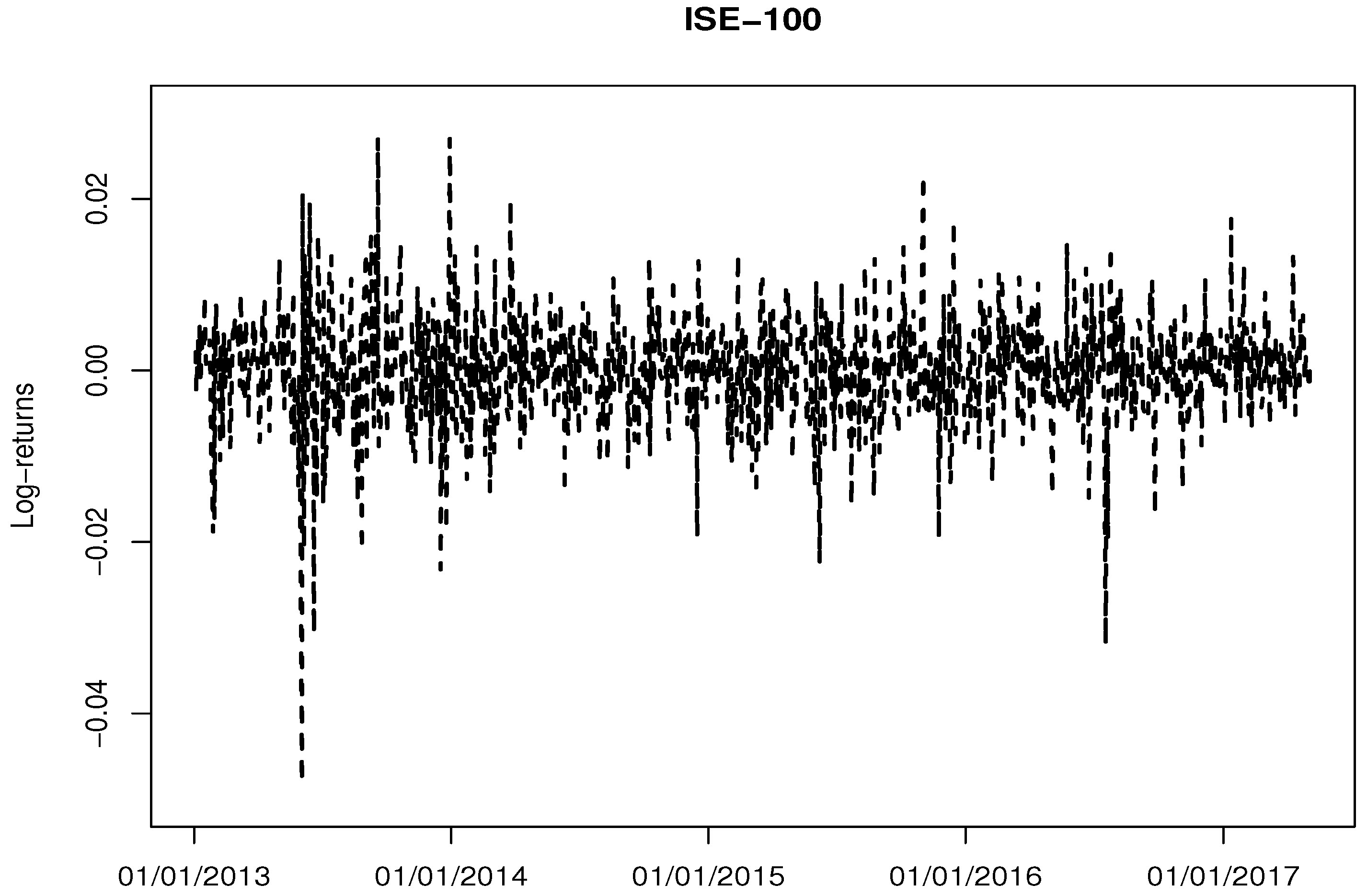
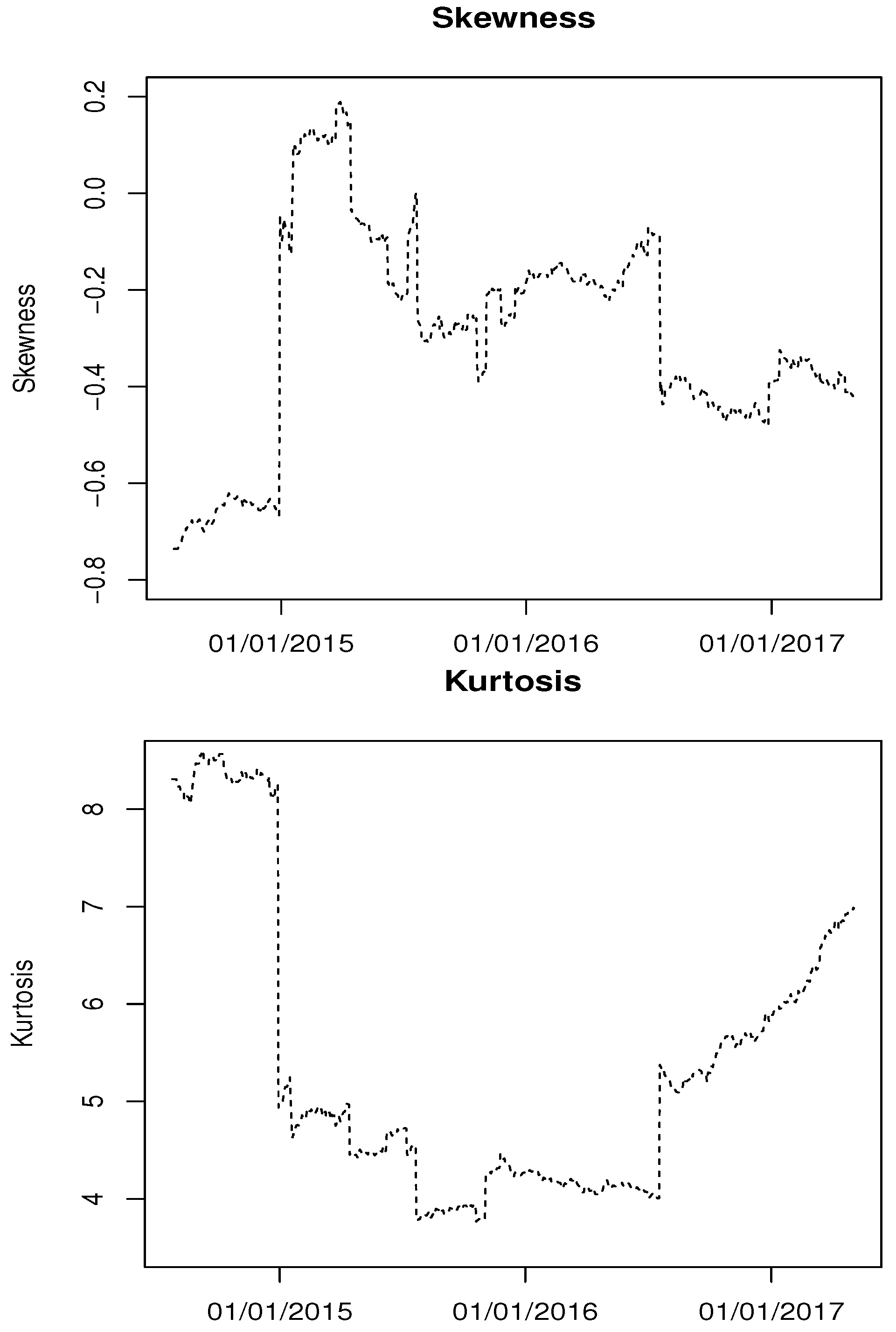
4.1. Data Description

To evaluate the performance of FHS models in terms of accuracy of VaR forecasts, ISE-100 index of Turkey is used. The used time series data contains 1092 daily log-returns from 3 January 2013 to 4 May 2017. The descriptive statistics of the log-returns of ISE-100 index are given in

Table 1. Summary statistics for the ISE-100 index.

ISE-100
Number of observations	1092
Minimum	−0.048
Maximum	0.027
Mean	$6.6\times {10}^{-5}$
Median	$2\times {10}^{-4}$
Std. Deviation	0.006
Skewness	−0.603
Kurtosis	4.957
Jarque-Bera	1190.970 (p <0.001)

.

Table 1 shows that the mean return is closed to 0. The results of the Jarque-Bera test prove that the null hypothesis of normality is rejected at any level of significance. It shows strong evidence for high excess kurtosis and negative skewness. Thus, it is clear that log return of ISE-100 index has non-normal characteristics, excess kurtosis, and fat tails. Figure 1 displays the daily log-returns of ISE-100 index.

Figure 2 displays the time-varying skewness and kurtosis of ISE-100. For Figure 2, window length is determined as 392 and the rolling window procedure is used. Based on Figure 2, it is clear that skewness and kurtosis of ISE-100 index exhibit great variability across the time.

The benchmark model, GARCH(1,1), is estimated with six different innovation distributions: Normal, SN, Student’s-t, ST, GED and SGED.

Table 2. In-sample performance of GARCH models under skewed and fat-tailed innovation distributions.

Parameters	Normal	Student-T	ST	SN	GED	SGED
$\mu$	$5.24\times {10}^{-4}$	$5.67\times {10}^{-4}$	$8.56\times {10}^{-4}$	$4.05\times {10}^{-4}$	$5.67\times {10}^{-4}$	$3.51\times {10}^{-4}$
	$3.41\times {10}^{-4}$	$3.04\times {10}^{-4}$	$3.60\times {10}^{-4}$	$3.34\times {10}^{-4}$	$3.77\times {10}^{-4}$	$3.26\times {10}^{-4}$
$\omega$	$3.69\times {10}^{-6}$	$2.01\times {10}^{-6}$	$2.27\times {10}^{-6}$	$3.65\times {10}^{-6}$	$2.72\times {10}^{-6}$	$2.63\times {10}^{-6}$
	$1.50\times {10}^{-6}$	$1.53\times {10}^{-6}$	$6.71\times {10}^{-6}$	$1.73\times {10}^{-6}$	$1.66\times {10}^{-6}$	$1.57\times {10}^{-6}$
${\gamma }_1$	0.1194	0.0759	0.1510	0.1460	0.0930	0.0873
	0.0413	0.0336	0.2940	0.0560	0.0393	0.0353
${\gamma }_2$	0.8234	0.8908	0.8240	0.7950	0.8600	0.8650
	0.0449	0.0485	0.3130	0.0662	0.0518	0.0486
$\nu$	-	4.7490	4.8760	-	1.2020	-
	-	1.1600	0.5620	-	0.1040	-
$\lambda$	-	-	−0.2750	−1.5050	-	0.8860
	-	-	2.4260	0.2630	-	0.0440
$\kappa$	-	-	-	-	-	1.2200
	-	-	-	-	-	0.1093
$-\ell$	−1381.1100	−1405.003	−1402.2630	−1388.1800	−1401.0600	−1402.7300

shows the estimated parameters of GARCH models. The rugarch package in R software is used to obtain parameter estimation of normal, Student’s-t, GED and SGED models. The constrOptim function in R software is used to minimize negative log-likelihood functions of GARCH-ST and GARCH-SN models.

Based on Table 2, we conclude that GARCH-T and GARCH-SGED models have the lower log-likelihood value among others. Since GARCH-T model has the lowest log-likelihood value, it could be chosen as best model for in-sample period. Table 2 also shows that the conditional variance parameters ${\gamma }_2$ are highly significant for all GARCH models.

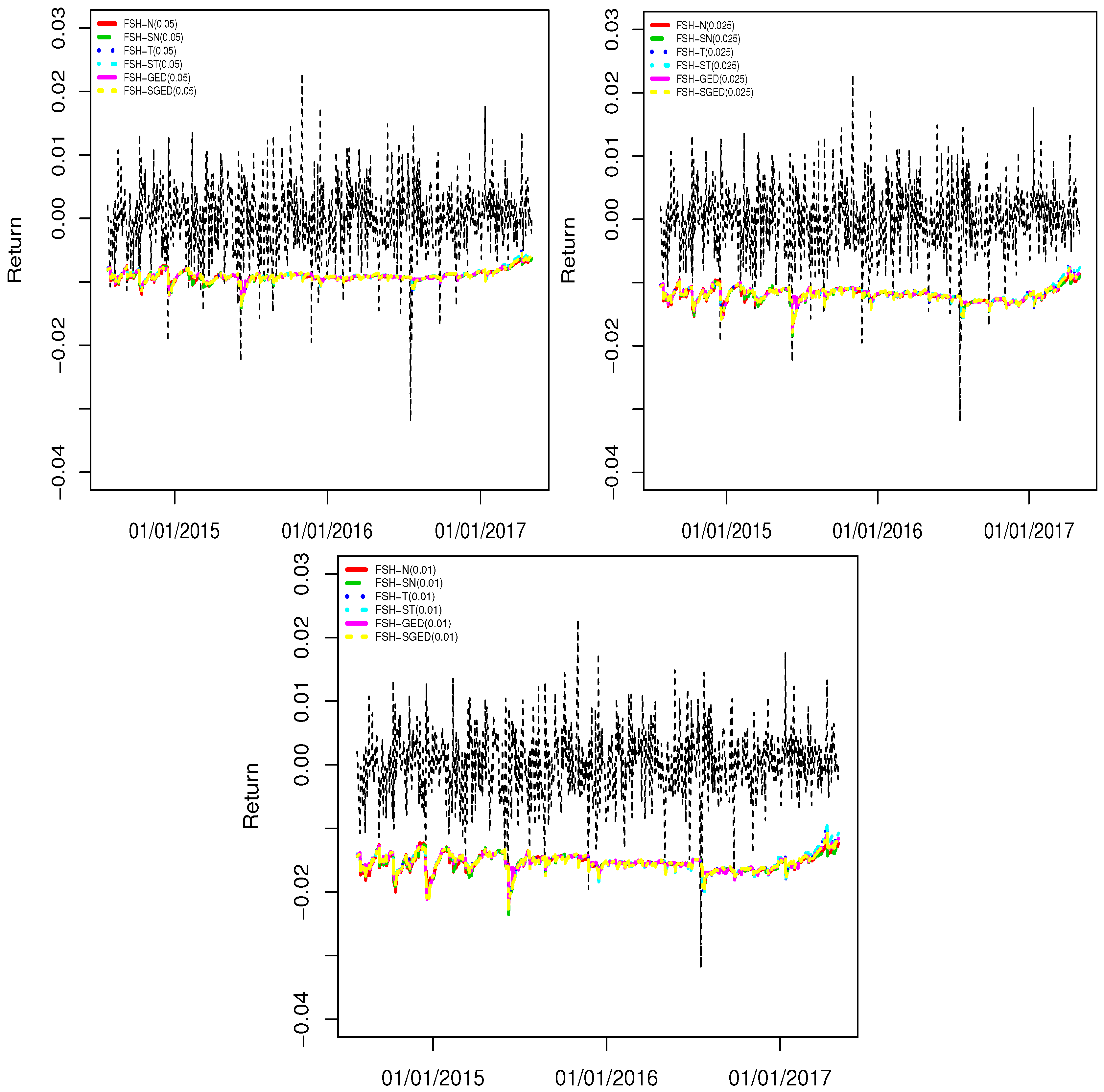
4.2. Backtesting Results

In this subsection, rolling window estimation procedure is used to estimate parameters of GARCH models. Then, VaR forecasts of FHS models are obtained by using estimated parameters of GARCH models, one-day-ahead forecasts of conditional mean and conditional variance and standardized residuals extracted from estimated GARCH models. Rolling window estimation produce allows us to capture time-varying characteristics of the time series in different time periods. Window length is determined as 392 and next 700 daily returns are used to evaluate the out of sample performance of VaR models.

Table 3. Backtesting results of FHS models for long position ($p=0.05$, $p=0.025$, and $p=0.01$).

p = 0.05
Models	Mean VaR (%)	N. Of Vio.	Failure Rate	LR-uc	LR-cc	DQ
FSH-N	−0.910	29	0.041	1.146 (0.284)	1.186 (0.552)	4.586 (0.710)
FSH-SN	−0.911	29	0.041	1.146 (0.284)	1.186 (0.552)	4.545 (0.715)
FSH-T	−0.897	32	0.046	0.278 (0.597)	0.459 (0.794)	2.996 (0.885)
FSH-GED	−0.899	30	0.043	0.788 (0.374)	0.863 (0.649)	4.041 (0.775)
FSH-SGED	−0.904	30	0.043	0.788 (0.374)	0.863 (0.649)	4.255 (0.749)
FSH-ST	−0.897	32	0.046	0.278 (0.597)	0.459 (0.794)	3.187 (0.867)
p = 0.025
Models	Mean VaR (%)	N. Of Vio.	Failure Rate	LR-uc	LR-cc	DQ
FSH-N	−1.193	20	0.029	0.350 (0.554)	0.630 (0.729)	6.820 (0.448)
FSH-SN	−1.196	20	0.029	0.350 (0.554)	0.630 (0.729)	6.805 (0.449)
FSH-T	−1.177	20	0.029	0.350 (0.554)	0.630 (0.729)	4.056 (0.773)
FSH-GED	−1.179	20	0.029	0.350 (0.554)	0.630 (0.729)	4.579 (0.711)
FSH-SGED	−1.187	20	0.029	0.350 (0.554)	0.630 (0.729)	5.102 (0.647)
FSH-ST	−1.177	20	0.029	0.350 (0.554)	0.630 (0.729)	4.051 (0.774)
Models	Mean VaR (%)	N. Of Vio.	Failure Rate	LR-uc	LR-cc	DQ
FSH-N	−1.546	9	0.013	0.529 (0.466)	0.764 (0.682)	15.479 (0.030)
FSH-SN	−1.549	9	0.013	0.529 (0.466)	0.764 (0.682)	16.338 (0.022)
FSH-T	−1.526	9	0.013	0.529 (0.466)	0.764 (0.682)	13.185 (0.067)
FSH-GED	−1.530	8	0.011	0.137 (0.710)	0.323 (0.851)	16.115 (0.024)
FSH-SGED	−1.538	9	0.013	0.529 (0.466)	0.764 (0.682)	14.620 (0.041)
FSH-ST	−1.526	9	0.013	0.529 (0.466)	0.764 (0.682)	12.893 (0.075)

p values of LR-uc, LR-cc and DC tests are presented in parentheses.

shows the backtesting results for FHS-N, FHS-T, FHS-ST, FHS-SN, FHS-GED and FHS-SGED models. The two step decision making procedure is applied to decide the best VaR model. In first step, the performance of VaR models are evaluated according to results of $L{R}_{u}c$, $L{R}_{c}c$ and $DC$ tests. In second step, the models, achieved to pass these three backtest, considered as accurate model and obtained the results of loss functions of these VaR models. Finally, the lowest values of loss functions indicate the best VaR models.

Table 4. Loss functions results of FHS models for long position ($p=0.05$, $p=0.025$, and $p=0.01$).

p = 0.05
Models	ARLF	Min.-Max. ARLF	UL	Min.-Max. UL	FLF	Min.-Max. FLF
FSH-N	0.0172063	($1\times {10}^{-4}$, 5.133)	−0.0179110	(−2.265, −0.010)	0.0283988	($1\times {10}^{-4}$, 5.133)
FSH-SN	0.0171900	($1\times {10}^{-4}$, 5.121)	−0.0178643	(−2.263, −0.011)	0.0283877	($1.37\times {10}^{-4}$, 5.121)
FSH-T	0.0173740	($5.84\times {10}^{-8}$, 5.150)	−0.0181385	(−2.269, $-2\times {10}^{-4}$)	0.0284271	($5.84\times {10}^{-8}$, 5.150)
FSH-GED	0.0172983	($1.89\times {10}^{-6}$, 5.135)	−0.0180858	(−2.266, −0.001)	0.0283820	($1.89\times {10}^{-6}$, 5.135)
FSH-SGED	0.0173162	($2.05\times {10}^{-5}$, 5.145)	−0.0179867	(−2.268, −0.004)	0.0284463	($2.05\times {10}^{-5}$, 5.145)
FSH-ST	0.0173437	($9.28\times {10}^{-6}$, 5.127)	−0.0181591	(−2.264, −0.003)	0.0283897	($9.28\times {10}^{-6}$, 5.127)
p = 0.025
Models	ARLF	Min.-Max. ARLF	UL	Min.-Max. UL	FLF	Min.-Max. FLF
FSH-N	0.0097984	(0.003, 3.896)	−0.0108364	(−1.974, −0.058)	0.0228029	(0.003, 3.896)
FSH-SN	0.0097622	(0.001, 3.863)	−0.0107498	(−1.965, −0.033)	0.0227883	(0.001, 3.863)
FSH-T	0.0098350	(0.002, 3.886)	−0.0108600	(−1.971, −0.049)	0.0226889	(0.002, 3.886)
FSH-GED	0.0097898	(0.004, 3.876)	−0.0108694	(−1.968, −0.063)	0.0226529	(0.004, 3.876)
FSH-SGED	0.0098099	(0.002, 3.893)	−0.0107848	(−1.973, −0.040)	0.0227502	(0.002, 3.893)
FSH-ST	0.0098287	(0.002, 3.884)	−0.0108752	(−1.971, −0.049)	0.0226755	(0.002, 3.884)
p = 0.01
Models	ARLF	Min.-Max. ARLF	UL	Min.-Max. UL	FLF	Min.-Max. FLF
FSH-N	0.0052475	($7.17\times {10}^{-5}$, 2.885)	−0.0051635	(−1.698, −0.008)	0.0212668	($7.17\times {10}^{-5}$, 2.885)
FSH-SN	0.0052483	( $8.22\times {10}^{-5}$, 2.893)	−0.0051776	(−1.700, −0.009)	0.0213011	($8.22\times {10}^{-5}$, 2.893)
FSH-T	0.0052399	($1\times {10}^{-4}$, 2.914)	−0.0051979	(−1.707, −0.011)	0.0210625	($1.15\times {10}^{-4}$, 2.914)
FSH-GED	0.0052125	($3\times {10}^{-4}$, 2.882)	−0.0051546	(−1.697, −0.017)	0.0210964	($2.81\times {10}^{-4}$, 2.882)
FSH-SGED	0.0052148	($4\times {10}^{-4}$, 2.883)	−0.0051849	( −1.697, −0.019)	0.0211543	($3.98\times {10}^{-4}$, 2.883)
FSH-ST	0.0052135	($3.32\times {10}^{-5}$, 2.895)	−0.0051634	(−1.701, −0.006)	0.0210319	($3.32\times {10}^{-5}$, 2.895)

p values of LR-uc and LR-cc tests are presented in parentheses.

shows that all FHS models perform well based on the results of $L{R}_{uc}$, $L{R}_{cc}$ and $DC$ tests results at $p=0.05$ ad $p=0.025$ levels. However, FHS model with Student’s-t and ST innovation distributions provide better VaR forecasts than other competitive models at $p=0.01$ level based on the result of $DC$ test. Therefore, it can be concluded that FHS model specified under skewed and fat-tailed innovation distributions provides more accurate VaR forecasts especially for high quantiles.

Even if FHS models have similar results in view of $L{R}_{uc}$, $L{R}_{cc}$ and $DC$ results, they have different failure rates and forecast errors. Loss functions are useful to compare VaR models with their forecast errors. Based on the ARLF, UL and FLF results, we conclude following results: (i) FHS-SN is the best performed model at $p=0.05$ and $p=0.025$ levels according to ARLF and UL criteria. Based on the FLF results, FHS-GED model has the lowest excess capital value than other models at $p=0.05$ and $p=0.025$ levels. Therefore, FHS-GED model could be chosen as best model for $p=0.05$ and $p=0.025$ levels; (ii) Based on the three backtesting results, FHS-T and FHS-ST models provide the most accurate VaR forecasts among others at $p=0.01$ level. According to loss functions results, it is easy to see that FHS-ST model has lower values of ARLF, UL and FLF results than FHS-T model. Therefore, FHS-ST model could be chosen as the best model for $p=0.01$ model.

Figure 3 displays the VaR forecasts of FHS models specified under six innovation distributions. As seen in Figure 3, the assumption on innovation process does not affect the VaR forecasts of FHS model soulfully. However, the GED and ST distributions could be preferable to reduce the forecast error of the FHS model.

5. Conclusions

In this study, we investigate FHS models with skewed and fat-tailed innovation distributions both theoretically and empirically. For this aim, we use Normal, Student’s-t, ST, SN, GED and SGED as the innovation distributions. The empirical findings show that all of FHS models perform well based on the $L{R}_{uc}$, $L{R}_{cc}$ and $DC$ results at $p=0.05$ and $p=0.025$ levels. However, only two FHS model, FHS-T and FHS-ST models achieve to pass $L{R}_{uc}$, $L{R}_{cc}$ and $DC$ tests at $p=0.01$ level. Based on the results of loss functions, FHS-GED is the best performed model at $p=0.05$ and $p=0.025$ levels and FHS-ST model is the best performed model at $p=0.01$ level. We conclude that skewed and fat-tailed distributions are preferable to reduce the VaR forecast error of FHS models. We hope that the results given in this study will be useful for both researchers and practitioners.

References

1. Angelidis, Timotheos, Alexandros Benos, and Stavros Degiannakis. 2007. A robust VaR model under different time periods and weighting schemes. Review of Quantitative Finance and Accounting 28: 187–201. [Google Scholar] [CrossRef]
2. Azzalini, Adelchi. 1985. A class of distributions which includes the normal ones. Scandinavian Journal of Statistics 12: 171–78. [Google Scholar]
3. Azzalini, Adelchi, and Antonella Capitanio. 2003. Distributions generated by perturbation of symmetry with emphasis on a multivariate skew t-distribution. Journal of the Royal Statistical Society: Series B (Statistical Methodology) 65: 367–89. [Google Scholar] [CrossRef]
4. Barone-Adesi, Giovanni, Kostas Giannopoulos, and Les Vosper. 1999. VaR without correlations for nonlinear portfolios. Journal of Futures Markets 19: 583–602. [Google Scholar] [CrossRef]
5. Barone-Adesi, Giovanni, and Kostas Giannopoulos. 2001. Non parametric var techniques. myths and realities. Economic Notes 30: 167–81. [Google Scholar] [CrossRef]
6. Bollerslev, Tim. 1986. Generalized autoregressive conditional heteroskedasticity. Journal of Econometrics 31: 307–27. [Google Scholar] [CrossRef]
7. Bollerslev, Tim. 1987. A conditionally heteroskedastic time series model for speculative prices and rates of return. The Review of Economics and Statistics 69: 542–47. [Google Scholar] [CrossRef]
8. Christoffersen, Peter F. 1998. Evaluating interval forecasts. International Economic Review 39: 841–62. [Google Scholar] [CrossRef]
9. Dumitrescu, Elena-Ivona, Christophe Hurlin, and Vinson Pham. 2012. Backtesting value-at-risk: from dynamic quantile to dynamic binary tests. Finance 33: 79–112. [Google Scholar]
10. Engle, Robert F., and Simone Manganelli. 2004. CAViaR: Conditional autoregressive value at risk by regression quantiles. Journal of Business & Economic Statistics 22: 367–81. [Google Scholar]
11. Hull, John, and Alan White. 1998. Incorporating volatility updating into the historical simulation method for value-at-risk. Journal of Risk 1: 5–19. [Google Scholar] [CrossRef]
12. Kupiec, Paul H. 1995. Techniques for verifying the accuracy of risk measurement models. The Journal of Derivatives 3: 73–84. [Google Scholar] [CrossRef]
13. Kuester, Keith, Stefan Mittnik, and Marc S. Paolella. 2006. Value-at-risk prediction: A comparison of alternative strategies. Journal of Financial Econometrics 4: 53–89. [Google Scholar] [CrossRef]
14. Lee, Ming-Chih, Jung-Bin Su, and Hung-Chun Liu. 2008. Value-at-risk in US stock indices with skewed generalized error distribution. Applied Financial Economics Letters 4: 425–31. [Google Scholar] [CrossRef]
15. Mögel, Benjamin, and Benjamin R. Auer. 2017. How accurate are modern Value-at-Risk estimators derived from extreme value theory? Review of Quantitative Finance and Accounting, 1–52. [Google Scholar]
16. Nelson, Daniel B. 1991. Conditional heteroscedasticity in asset returns: A new approach. Econometrica 59: 347–70. [Google Scholar] [CrossRef]
17. Omari, Cyprian Ondieki. 2017. A Comparative Performance of Conventional Methods for Estimating Market Risk Using Value at Risk. International Journal of Econometrics and Financial Management 5: 22–32. [Google Scholar]
18. Roy, Indrajit. 2011. Estimating Value at Risk (VaR) using Filtered Historical Simulation in the Indian capital market. Reserve Bank of India Occasional Papers 32: 81–98. [Google Scholar]
19. Sarma, Mandira, Susan Thomas, and Ajay Shah. 2003. Selection of Value-at-Risk models. Journal of Forecasting 22: 337–58. [Google Scholar] [CrossRef]
20. Ziggel, Daniel, Tobias Berens, Gregor N. F. Weiß, and Dominik Wied. 2014. A new set of improved Value-at-Risk backtests. Journal of Banking & Finance 48: 29–41. [Google Scholar]
Figure 1. Daily log-returns of the ISE-100 index.
Jrfm 11 00007 g001
Figure 2. Time varying skewness and kurtosis plots of ISE-100 index.
Jrfm 11 00007 g002
Figure 3. Daily VaR forecast of GARCH models with different innovation distributions for 97.5% and 99% confidence levels.
Jrfm 11 00007 g003