Hierarchical Transmuted Log-Logistic Model: A Subjective Bayesian Analysis

Abstract

In this study, we propose to apply the transmuted log-logistic (TLL) model which is a generalization of log-logistic model, in a Bayesian context. The log-logistic model has been used it is simple and has a unimodal hazard rate, important characteristic in survival analysis. Also, the TLL model was formulated by using the quadratic transmutation map, that is a simple way of derivating new distributions, and it adds a new parameter $\lambda$, which one introduces a skewness in the new distribution and preserves the moments of the baseline model. The Bayesian model was formulated by using the half-Cauchy prior which is an alternative prior to a inverse Gamma distribution. In order to fit the model, a real data set, which consist of the time up to first calving of polled Tabapua race, was used. Finally, after the model was fitted, an influential analysis was made and excluding only $0.1\%$ of observations (influential points), the reestimated model can fit the data better.

1. Introduction

The genetic prepotency of cows is an important issue since the development of livestock is directly related to the growth of the food production. Brazilians institutes are concerned with the development of a particular race, the Tabapua, which was the first humped cattle developed in the country. Due to the economic results of this particular race, this study is twofold: present the TLL model and fit the times up to the first calving of the cows pointing characteristics of this race.

Proposed by Granzotto and Louzada-Neto (2014), the TLL model presents important characteristics of a good model: it is flexible, tractable, interpretable and simple. Following the Shaw and Buckley (2007) idea, this new distribution incorporates a new third parameter $\lambda$ that introduces skewness and preserve the moments of the baseline distribution. Several studies can be cited that proposed similar generalizations of survival models, see for example (Aryal and Tsokos 2009; Aryal and Tsokos 2011).

Due to good characteristics of the TTL model along with its simplicity (the main functions are analytically expressed) and the hazard properties (it has a larger range of choices for the shape of the hazard function most commonly observed in the survival analysis field), this paper present an application of the model in a Bayesian context.

In order to fit this new model, the subjective Bayesian analysis was used. For that, the half-Cauchy prior distribution, cited by several authors such as (Polson and Scott 2012; Gelman 2006), as an alternative prior to a inverse Gamma distribution, was used. Specially, Gelman (2006) made use of this particular prior for variance parameters in hierarchical models which is our case.

Furthermore, in order to provide an indication of bad model fitting or influential observations, an influential analysis was made, see for example (Ortega et al. 2003; Fachini et al. 2008).

The paper is organized as follows. The hierarchical log-logistic model built by using the half-Cauchy prior distribution is presented in Section 2. In Section 3 we presented an application by using a real data set on a polled Tabapua race time up to first calving data. An influence diagnostic was presented in Section 4 and the data set was re-analyzed refitting the model. Final remarks and conclusions are presented in Section 5.

2. Hierarchical TLL Model

Proposed by Granzotto and Louzada-Neto (2014), the TLL is a generalization of the log-logistic model containing the baseline model as a particular case (for log-logistic distribution see (Bennett 1983; Chen et al. 2001)). Tractable, Interpretable and flexible enough, the new construction can be used to analyze more complex dataset, introducing skew to a base distribution and preserving its moments. Let X be a nonnegative random variable denoting the lifetime of an individual in some population then, the probability density function (pdf) and the cumulative function of the TLL distribution are respectively given by

$$\begin{array}{ccc}\hfill f\left(x\right)& =& \frac{e^{\mu }\beta x^{\beta -1}\left[\left(1+e^{\mu }{x}^{\beta }\right)-\lambda \left(e^{\mu }{x}^{\beta }-1\right)\right]}{{\left(1+e^{\mu }{x}^{\beta }\right)}^3}.\hfill \end{array}$$

(1)

and

$$\begin{array}{ccc}\hfill F\left(x\right)& =& \frac{e^{\mu }{x}^{\beta }}{{\left(1+e^{\mu }{x}^{\beta }\right)}^2}\left(1+e^{\mu }{x}^{\beta }+\lambda \right).\hfill \end{array}$$

(2)

where $\beta >0$, $\mu \in \mathbb{R}$ and $-1\le \lambda \le 1$. Since the distribution was proposed to model experiments in reliability analysis, Figure 1 presents several examples of survival, probability density and hazard rate functions for different values of the parameters.

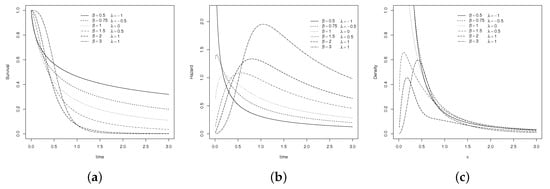
Figure 1. Transmuted model curves: (a) Survival, (b) hazard and (c) probability density function.

According to Chen and Ibrahim (2006), one of most common ways of combining several sources of information is though hierarchical modeling. Thus, the authors show us the relationship between the power prior and hierarchical models using as example the regression models.

Also, Gelman (2006) show us that several studies by using multilevel models are central to modern Bayesian statistics for both conceptual and practical reasons. The authors suggest to use the half-t family as a prior distribution for variance parameters such the half-Cauchy distribution, that is a special conditionally-conjugate folded-noncentral-t family case of prior distributions for parameters that represent the discrepancy. Even though several studies use the half-Cauchy prior for scale parameter (see for example Polson and Scott 2012), Gelman (2006) used this prior not for scale but for variance parameters and illustrated serious problems with the inverse-Gamma prior which is the most commonly used prior for variance component, see Daniels and Daniels (1998).

In this paper we proposed to use the hierarchical models in two levels, for that, suppose the hierarchical model given as $[X|\mu ,\beta ,\lambda ]\sim f(x|\mu ,\beta ,\lambda )$, $\mu |{\sigma }^2\sim {\pi }_{\mu }(\mu |{\sigma }^2)$, $\beta |\theta \sim {\pi }_{\beta }(\beta |\theta )$, $\lambda \sim {\pi }_{\lambda }\left(\lambda \right)$, ${\sigma }^2\sim {\psi }_{\sigma }\left({\sigma }^2\right)$ and $\theta \sim {\psi }_{\theta }\left(\theta \right)$. The posterior distribution can be constructed as following.

Proposition 1.

Let us suppose that, in the first stage, we considered a class Γ of priors that led to following

$$\begin{array}{ccc}\hfill \Gamma & =& \left\{\left.\pi (\mu ,\beta ,\lambda |{\sigma }^2,\theta ):\pi (\mu ,\beta ,\lambda |{\sigma }^2,\theta )={\pi }_{\mu }\left(\mu \right|{\sigma }^2){\pi }_{\beta }\left(\beta \right|\theta ){\pi }_{\lambda }\left(\lambda \right)\right|\right.\hfill \\ & & {\pi }_{\mu }\mathrm{being}\mathrm{N}(\tau ,{\sigma }^2),(\tau ,{\sigma }^2)\in \mathbb{R}\times {\mathbb{R}}^{+};{\pi }_{\beta }\mathrm{being}\mathrm{HC}\left(\theta \right),\theta \in {\mathbb{R}}^{+};\hfill \\ & & \left.{\pi }_{\lambda }\mathrm{being}\mathrm{U}(a,b),(a,b)\in \mathbb{R}\times \mathbb{R},a<b\right\}.\hfill \end{array}$$

Also, the second stage (sometimes called a hyperprior), would consist of putting a prior distribution ${\psi }_k(·)$ on the hyperparameters ${\sigma }^2$ and θ where

$$\begin{array}{ccc}\hfill {\Psi }& =& \left\{\psi ({\sigma }^2,\theta ):\psi ({\sigma }^2,\theta )={\psi }_{{\sigma }^2}\left({\sigma }^2\right){\psi }_{\theta }\left(\theta \right){\psi }_{{\sigma }^2}\mathrm{being}\mathrm{Gamma}(\alpha ,\zeta ),\right.\hfill \\ & & (\alpha ,\zeta )\in {\mathbb{R}}^{+}\times {\mathbb{R}}^{+};{\psi }_{\beta }\mathrm{being}\mathrm{Gamma}(\eta ,\vartheta ),(\eta ,\vartheta )\in {\mathbb{R}}^{+}\times {\mathbb{R}}^{+};\hfill \\ & & \left.\alpha ,\zeta ,\eta ,\vartheta \mathrm{are}\mathrm{known}\mathrm{and}\mathrm{does}\mathrm{not}\mathrm{depend}\mathrm{on}\mathrm{any}\mathrm{other}\mathrm{hyperparameter}\right\}.\hfill \end{array}$$

Thus, the hyerarchical log-logistic posterior distribution is written as

$$\begin{array}{ccc}\hfill \pi (\mu ,\beta ,\lambda |\mathbf{x})& \propto & \frac{e^{\mu }\beta \theta }{\sigma }\left[x^{\beta +\alpha +\eta -3}\frac{\left[(1+e^{\mu }{x}^{\beta })-\lambda (e^{\mu }{x}^{\beta }-1)\right]}{{(1+e^{\mu }{x}^{\beta })}^3}\right]\hfill \\ & & \times exp\left\{-\left(\zeta +\vartheta +\frac{x}{2{\sigma }^2}\right)\right\}.\hfill \end{array}$$

(3)

Proof. 

The demonstration is direct.

Note that, the $\beta$ parameter is supposed to be a half-Cauchy distribution which probability density function given by

$$f\left(x\right)=\frac{2\theta }{\pi \left(x^2+{\theta }^2\right)},x>0,\theta >0,$$

(4)

where $\theta$ is a scale parameter which has a broad peak at zero and, in limit, $\theta \to \infty$ this becomes a uniform prior density. However, large finite values for $\theta$ represent prior distributions which we call “weakly informative”. For example, Gelman (2006) show us that, for $\theta =25$, the half-Cauchy is nearly flat although it is not completely. ☐

3. Application to Real Data

Founded in 70’s, the Brazilian Agricultural Research Corporation (Embrapa) is under the aegis of the Brazilian Ministry of Agriculture, Livestock, and Food Supply. Since the foundation, they have taken on the challenge to develop a genuinely Brazilian model of tropical livestock (and agriculture as well), to keep increasing the production of food. As a result of the intense research work, the beef and pork supply were quadrupled, helping the Brazilian food to one of the world’s largest food producers and exporters.

One of the special research is related to the genetic prepotency of cows whereas the economic results is directly related to beef cattle, see for example Pereira (2000). Granzotto and Louzada-Neto (2014) study the Tabapua race time up to first calving of $\mathrm{17,026}$ animals observed from 1983 to 2007, held at Embrapa. Firstly, as the minimum observed calving was 721 days, we subtract this amount of the observed times and the distribution of the first calving times can be observed in the Figure 2b.

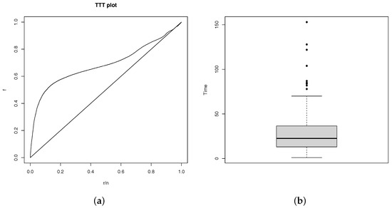
Figure 2. (a) TTT Plot and (b) boxplot of times.

Also, the TTT plot, presented in Figure 2a shows the possible unimodal hazard rate as it is concave, convex and then concave again, see for example Barlow and Campo (1975).

After initial analysis, we are considering the hierarchical TLL model, as we specify in Section 2, to fit the data. The posterior samples were generated by the Metropolis-Hastings technique. Three chains of the dimension $\mathrm{100,000}$ was considered for each parameter, discarding the first 10,000 iterations (in order to eliminate the effect of the initial values), a lag size 10 was used to avoid the correlation problems, resulting in a final sample size 10,000. The posterior summaries for $\mu ,\beta ,\lambda ,{\sigma }^2$ and $\theta$ are present in Table 1 and the $95\%$ credible intervals by considering the priors above-mentioned can be seem in Table 2.

Table 1. Posterior model summary of the hierarchical TLL model parameters.

Parameter	Mean	Standard Deviation	Percentiles
			25%	50%	75%
$\mu$	$-17.865$	$0.138$	$-17.958$	$-17.871$	$-17.775$
$\beta$	$3.043$	$0.022$	$3.029$	$3.044$	$3.058$
$\lambda$	$-0.815$	$0.012$	$-0.823$	$-0.815$	$-0.807$
${\sigma }^2$	$900.100$	$822.500$	$333.800$	$640.400$	$1208.100$
$\theta$	$198.800$	$195.100$	$60.171$	$139.800$	$273.400$

Table 2. 95% Credible Interval of parameters estimated.

Parameter	Equal-Tail Interval		HPD Interval
$\mu$	$-18.123$	$-17.576$	$-18.118$	$-17.571$
$\beta$	$2.997$	$3.085$	$2.997$	$3.084$
$\lambda$	$-0.838$	$-0.791$	$-0.838$	$-0.790$
${\sigma }^2$	$96.474$	$3044.600$	$37.837$	$2516.300$
$\theta$	$5.395$	$733.800$	$0.008$	$594.800$

The convergence of the chain was verified by Gelman and Rubin’s convergence diagnostic criterion, see for example (Gelman and Rubin 1992), which demonstrate that these criteria is satisfied (Table 3). Also, the convergence can be seem in Figure 3a–j.

Table 3. Gelman and Rubin’s criterion to verify the parameters convergence of the hierarchical TLL distribution.

Parameter	Estimate	Upper Bound
$\mu$	$1.0085$	$1.0060$
$\beta$	$1.0082$	$1.0057$
$\lambda$	$1.0020$	$1.0017$
${\sigma }^2$	$1.0016$	$1.0019$
$\theta$	$1.0004$	$1.0009$

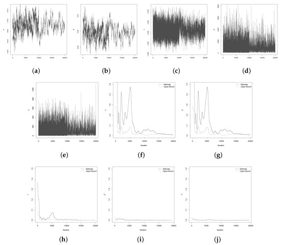
Figure 3. Traceplots and convergence plots, respectively, for: (a,f): $\mu$; (b,g): $\beta$; (c,h): $\lambda$; (d,i): ${\sigma }^2$ and; (e,j): $\theta$.

Also, the marginal posterior densities for $\mu$, $\beta$ and $\lambda$, respectively, can be analyzed by the Figure 4a–e.

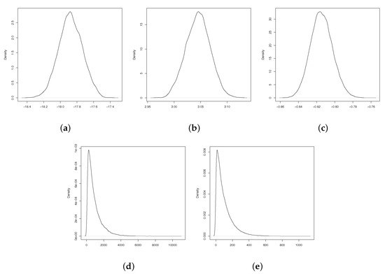
Figure 4. Marginal posteriors densities for: (a) $\mu$, (b) $\beta$, (c) $\lambda$, (d) ${\sigma }^2$ and (e) $\theta$.

After estimate and analyze the convergence of the model, Figure 5a,b show us, respectively, the hazard estimate curve, with the ${\widehat{T}}_{max}$ and the $T_{max}$ $95\%$ confidence interval; the survival curves estimated vs empirical and the histograma which are possible to see how well it fits a set of observations.

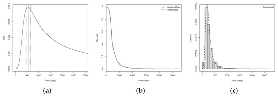
Figure 5. (a) hazard estimate curve, with the ${\widehat{T}}_{max}$ and the $T_{max}$ $95\%$ confidence interval, (b) survival curves and (c) histogram.

Considering the hyerarchical TLL fitting, the ${\widehat{T}}_{max}$ is equals to $546.77$ days ($18.23$ months) and its $95\%$ confidence interval is given by IC$\left[T_{max},95\%\right]=\left(460.04;652.86\right)$ days (see Figure 5a). Furthermore, the median time up to first calving is equals to $452.48$ days (or approximately $15.08$ months), and the mean of time is $540.13$ days (or approximately 18 months), with standard deviation equals to $13.34$ months.

4. Influence Analysis

In this section we present an analysis of global influence for the data set given, using the TLL model in a bayesian context.

In few words, the influence analysis is a case-deletion, that we study the effect of withdraw of the ith element sampled. Several measures of global influence analysis are presented in the literature. In this study we are considering two: the generalized Cook’s distance (CD) and the likelihood difference (LD). The first one, CD, defined as the standard norm of ${\mathbf{\zeta }}_i=({\mu }_i,{\beta }_i,{\lambda }_i,{\sigma }_i^2,{\theta }_i)$ and $\widehat{\mathbf{\zeta }}=(\widehat{\mu },\widehat{\beta },\widehat{\lambda },{\widehat{\sigma }}^2,\widehat{\theta })$, and the LD are given, respectively, by

$$C{D}_i\left(\mathbf{\zeta }\right)={\left[\begin{array}{c}{\mathbf{\zeta }}_i-\widehat{\mathbf{\zeta }}\end{array}\right]}^T\left[-\ddot{L}\left(\mathbf{\zeta }\right)\right]\left[\begin{array}{c}{\mathbf{\zeta }}_i-\widehat{\mathbf{\zeta }}\end{array}\right],$$

(5)

and

$$L{D}_i(\mathbf{\zeta })=2\{l(\widehat{\mathbf{\zeta }})-l({\mathbf{\zeta }}_i)\}.$$

(6)

According to Lee et al. (2006), $\ddot{L}\left(\mathbf{\zeta }\right)$ can be approximated by the estimated covariance and variance matrix. Some possible influence points are identified in the LD plot, Figure 6.

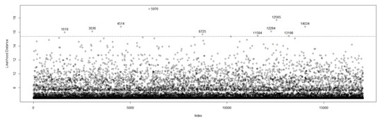
Figure 6. Likelihood distance.

Furthermore, the impact of the identified influential points should be measured. For that, we consider the relative changes that can be measured as ${\mathrm{RC}}_{{\zeta }_j}=\left|\frac{{\widehat{\zeta }}_j-{\widehat{\zeta }}_{j\left(I\right)}}{{\widehat{\zeta }}_j}\right|\times 100\%,j=1,\dots ,p+1$, where ${\widehat{\zeta }}_{j\left(I\right)}$ denotes the MLE of ${\zeta }_j$ after the set I of observations has been removed.

Three measures of influential observations are considered: TRC is the total relative changes, MRC the maximum relative changes and LD the likelihood displacement, see for example (Lee et al. 2006; Granzotto and Louzada-Neto 2014). Table 4 presents the values when we withdrew from 0.01 to 5% of the outstand identified points in Figure 6.

Table 4. RC (in %) and the corresponding TRC, MRC and LD${}_{\left(I\right)}$.

Removed Case	Parameter	RC	TRC	MRC	LD${}_{\left(\mathit{I}\right)}$
Identify Points	$\mu$	$8.271$	$86.438$	$68.336$	$142$
	$\beta$	$5.142$
	$\lambda$	$68.336$
	${\sigma }_2$	$2.877$
	$\theta$	$1.811$
0.1%	$\mu$	$0.844$	$3.598$	$1.358$	$217$
	$\beta$	$0.818$
	$\lambda$	$0.123$
	${\sigma }_2$	$0.456$
	$\theta$	$1.358$
0.5%	$\mu$	$2.098$	$8.634$	$3.219$	$949$
	$\beta$	$2.073$
	$\lambda$	$0.098$
	${\sigma }_2$	$1.144$
	$\theta$	$3.219$
1%	$\mu$	$3.257$	$9.782$	$3.257$	$1821$
	$\beta$	$3.250$
	$\lambda$	$0.368$
	${\sigma }_2$	$1.700$
	$\theta$	$1.207$
2%	$\mu$	$5.843$	$17.064$	$5.855$	$3519$
	$\beta$	$5.855$
	$\lambda$	$0.393$
	${\sigma }_2$	$2.911$
	$\theta$	$2.062$
3%	$\mu$	$8.096$	$22.086$	$8.162$	$5178$
	$\beta$	$8.162$
	$\lambda$	$1.460$
	${\sigma }_2$	$3.111$
	$\theta$	$1.258$
4%	$\mu$	$10.458$	$28.558$	$10.547$	$6775$
	$\beta$	$10.547$
	$\lambda$	$0.785$
	${\sigma }_2$	$6.566$
	$\theta$	$0.201$
5%	$\mu$	$12.463$	$34.232$	$12.627$	$8383$
	$\beta$	$12.627$
	$\lambda$	$2.160$
	${\sigma }_2$	$6.277$
	$\theta$	$0.704$

By considering the RC’s, 10 most influential points were withdrew and the model was re-fitted. Again, by using the Metropolis-Hastings technique we generated a chain of $\mathrm{100,000}$ observations, burn in of $\mathrm{10,000}$ and lag 10, resulting in a final sample size $\mathrm{10,000}$. Table 5 and Table 6 shows the posterior summaries and the $95\%$ credible intervals.

Table 5. Posterior model summary of the hierarchical TLL model parameters.

Removed Case	Parameter	Mean	Standard Deviation	Percentiles
				25%	50%	75%
Identify Points	$\mu$	$-19.343$	$1.269$	$-20.522$	$-20.327$	$-17.975$
	$\beta$	$3.200$	$0.130$	$3.062$	$3.285$	$3.319$
	$\lambda$	$-0.258$	$0.519$	$-0.813$	$0.153$	$0.232$
	${\sigma }^2$	$926.00$	$840.30$	$348.70$	$664.10$	$1224.00$
	$\theta$	$202.40$	$204.70$	$59.08$	$139.20$	$282.00$
0.1%	$\mu$	$-18.016$	$0.129$	$-18.098$	$-18.015$	$-17.933$
	$\beta$	$3.068$	$0.021$	$3.055$	$3.068$	$3.082$
	$\lambda$	$-0.814$	$0.012$	$-0.822$	$-0.814$	$-0.806$
	${\sigma }^2$	$904.20$	$826.40$	$334.50$	$651.90$	$1207.20$
	$\theta$	$196.10$	$194.80$	$56.84$	$137.20$	$270.50$
0.5%	$\mu$	$-18.240$	$0.135$	$-18.336$	$-18.238$	$-18.146$
	$\beta$	$3.107$	$0.022$	$3.091$	$3.106$	$3.122$
	$\lambda$	$-0.816$	$0.012$	$-0.824$	$-0.816$	$-0.808$
	${\sigma }^2$	$910.40$	$842.80$	$339.00$	$643.80$	$1203.30$
	$\theta$	$205.20$	$203.70$	$61.83$	$142.40$	$284.10$
1%	$\mu$	$-18.447$	$0.131$	$-18.536$	$-18.441$	$-18.352$
	$\beta$	$3.142$	$0.021$	$3.127$	$3.142$	$3.157$
	$\lambda$	$-0.818$	$0.012$	$-0.826$	$-0.818$	$-0.810$
	${\sigma }^2$	$915.40$	$853.70$	$337.50$	$647.80$	$1221.70$
	$\theta$	$196.40$	$195.20$	$56.19$	$136.90$	$273.10$
2%	$\mu$	$-18.909$	$0.144$	$-19.007$	$-18.907$	$-18.811$
	$\beta$	$3.222$	$0.023$	$3.206$	$3.221$	$3.238$
	$\lambda$	$-0.818$	$0.013$	$-0.827$	$-0.818$	$-0.810$
	${\sigma }^2$	$926.30$	$826.60$	$353.60$	$667.40$	$1235.00$
	$\theta$	$202.90$	$199.40$	$60.53$	$143.40$	$279.70$
3%	$\mu$	$-19.312$	$0.142$	$-19.410$	$-19.304$	$-19.222$
	$\beta$	$3.292$	$0.023$	$3.277$	$3.291$	$3.308$
	$\lambda$	$-0.827$	$0.012$	$-0.835$	$-0.827$	$-0.819$
	${\sigma }^2$	$928.10$	$849.10$	$352.20$	$668.20$	$1215.20$
	$\theta$	$196.30$	$193.30$	$56.37$	$139.00$	$275.50$
4%	$\mu$	$-19.734$	$0.154$	$-19.834$	$-19.737$	$-19.641$
	$\beta$	$3.364$	$0.025$	$3.350$	$3.365$	$3.381$
	$\lambda$	$-0.821$	$0.013$	$-0.830$	$-0.821$	$-0.813$
	${\sigma }^2$	$959.20$	$858.50$	$365.20$	$698.70$	$1267.90$
	$\theta$	$198.40$	$195.60$	$58.00$	$137.50$	$277.00$
5%	$\mu$	$-20.092$	$0.175$	$-20.221$	$-20.093$	$-19.967$
	$\beta$	$3.428$	$0.028$	$3.407$	$3.428$	$3.448$
	$\lambda$	$-0.832$	$0.013$	$-0.842$	$-0.833$	$-0.824$
	${\sigma }^2$	$956.60$	$854.00$	$372.90$	$704.10$	$1259.10$
	$\theta$	$200.20$	$198.30$	$59.91$	$141.00$	$273.20$

Table 6. 95% Credible Interval of parameters estimated.

Removed Case	Parameter	Equal-Tail Interval		HPD Interval
Identify Points	$\mu$	$-20.709$	$-17.754$	$-20.713$	$-17.760$
	$\beta$	$3.026$	$3.351$	$3.027$	$3.352$
	$\lambda$	$-0.833$	$0.293$	$-0.837$	$0.284$
	${\sigma }^2$	$104.300$	$3096.600$	$43.226$	$2603.000$
	$\theta$	$5.211$	$746.000$	$0.143$	$601.600$
0.1%	$\mu$	$-18.2762$	$-17.7678$	$-18.2845$	$-17.7776$
	$\beta$	$3.0289$	$3.11$	$3.0283$	$3.1093$
	$\lambda$	$-0.8365$	$-0.7896$	$-0.8372$	$-0.7906$
	${\sigma }^2$	$94.0797$	$3151.6$	$40.6435$	$2574.8$
	$\theta$	$5.2045$	$728.6$	$0.1098$	$586.3$
0.5%	$\mu$	$-18.4967$	$-17.9843$	$-18.4981$	$-17.9863$
	$\beta$	$3.0654$	$3.1476$	$3.0664$	$3.1483$
	$\lambda$	$-0.8391$	$-0.7905$	$-0.84$	$-0.7918$
	${\sigma }^2$	$98.81$	$3143.7$	$28.4125$	$2605.9$
	$\theta$	$5.1449$	$745.1$	$0.0156$	$613.7$
1%	$\mu$	$-18.7121$	$-18.205$	$-18.7066$	$-18.2029$
	$\beta$	$3.103$	$3.1855$	$3.1015$	$3.1829$
	$\lambda$	$-0.8407$	$-0.793$	$-0.8421$	$-0.7948$
	${\sigma }^2$	$102.2$	$3172.8$	$34.7775$	$2578.2$
	$\theta$	$4.6184$	$727.6$	$0.0235$	$591.8$
2%	$\mu$	$-19.1832$	$-18.6319$	$-19.184$	$-18.6338$
	$\beta$	$3.1769$	$3.266$	$3.1779$	$3.2663$
	$\lambda$	$-0.8415$	$-0.7927$	$-0.8428$	$-0.7944$
	${\sigma }^2$	$106.2$	$3111.3$	$39.5096$	$2606.1$
	$\theta$	$5.4845$	$729.9$	$0.0306$	$600.2$
3%	$\mu$	$-19.5917$	$-19.0343$	$-19.5817$	$-19.0259$
	$\beta$	$3.247$	$3.3364$	$3.2482$	$3.3373$
	$\lambda$	$-0.8504$	$-0.8013$	$-0.851$	$-0.8023$
	${\sigma }^2$	$107.5$	$3224.1$	$30.9968$	$2597.3$
	$\theta$	$4.8582$	$710.8$	$0.0153$	$578.9$
4%	$\mu$	$-20.0252$	$-19.4068$	$-20.0321$	$-19.4161$
	$\beta$	$3.312$	$3.4113$	$3.3143$	$3.4124$
	$\lambda$	$-0.8458$	$-0.7955$	$-0.8459$	$-0.7958$
	${\sigma }^2$	111	$3307.1$	$50.2358$	$2671.5$
	$\theta$	$5.2325$	$734.3$	$0.0631$	$604.8$
5%	$\mu$	$-20.4078$	$-19.7676$	$-20.418$	$-19.7839$
	$\beta$	$3.3762$	$3.4789$	$3.3778$	$3.4802$
	$\lambda$	$-0.8572$	$-0.8055$	$-0.8581$	$-0.8066$
	${\sigma }^2$	119	$3273.2$	$56.2007$	$2652.8$
	$\theta$	$5.0109$	$743.8$	$0.0992$	$605.8$

Clearly, the most affected estimate parameter was $\lambda$ if we compare to the parameters estimated by using the original dataset. Further, withdrawing $0.1\%$ of sample, i.e., just 17 observations, we do not lose much information and also improve the fitted model, see Figure 7a–c, that show us the fitted model.

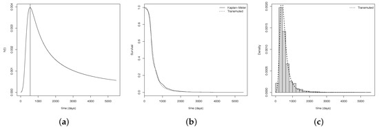
Figure 7. (a) Hazard estimate curve, with the ${\widehat{T}}_{max}$, (b) survival curves and (c) histogram.

5. Concluding Remarks

In this paper study the model propose by Granzotto and Louzada-Neto (2014), the TLL distribution, in a Bayesian context. The two levels hierarchical TLL model was formulated by using the half-Cauchy as a prior to the parameter of discrepancy.

Techniques of influential analysis were used to identify and measure the influence of the outstanding observed points. It is important to observe that the re-fitted model presents a reduction in the estimated likelihood value plus a reduction in the estimated standard deviation, which shortens the range of the confidence interval obtained for the most probable time up to first calving.

Finally, considering the final fitted model, the ${\widehat{T}}_{\max }$ changes to $547.71$ against $546.77$ days ($18.26$ months) and its $95\%$ confidence interval is given by IC$\left[T_{max},95\%\right]=\left(15.56;21.47\right)$ months. The median time up to first calving is equals to $452.41$ days (or approximately $15.08$ months), and the mean of time is $538.54$ days (or approximately $17.95$ months), with standard deviation equals to $13.11$ months.

References

- Aryal, Gokarna R., and Chris P. Tsokos. 2009. On the transmuted extreme value distribution with applications. Nonlinear Analysis 71: 1401–7. [Google Scholar] [CrossRef]
- Aryal, Gokarna R., and Chris P. Tsokos. 2011. Transmuted Weibull distribution: A generalization of the Weibull probability distribution. European Journal of Pure and Applied Mathematics 4: 89–102. [Google Scholar]
- Barlow, Richard E., and Rafael A. Campo. 1975. Total Time on Test Processes and Applications to Failure Data Analysis. Berkeley: California University Berkeley Operations Research Center. [Google Scholar]
- Bennett, Steve. 1983. Log-logistic regression models for survival data. Journal of the Royal Statistical Society Series C: Applied Statistics 32: 165–71. [Google Scholar] [CrossRef]
- Chen, Ming-Hui, Joseph G. Ibrahim, and Debajyoti Sinha. 2001. Bayesian Survival Analysis. Springer Series in Statistics; New York: Springer. [Google Scholar]
- Chen, Ming-Hui, and Joseph G. Ibrahim. 2006. The relationship between the power prior and hierarchical models. Bayesian Analysis 1: 551–74. [Google Scholar] [CrossRef]
- Daniels, Michael J. 1998. A prior for the variance in hierarchical models. The Canadian Journal of Statistics/La Revue Canadienne de Statistique 27: 567–78. [Google Scholar] [CrossRef]
- Fachini, B. Juliana, Edwin M. M. Ortega, and Francisco Louzada. 2008. Influence diagnostics for polyhazard models in the presence of covariates. Statistical Methods and Applications 17: 413–33. [Google Scholar] [CrossRef]
- Gelman, Andrew. 2006. Prior distributions for variance parameters in hierarchical models. Communications in Statistics. Theory and Methods 1: 515–33. [Google Scholar]
- Gelman, Andrew, and Donald B. Rubin. 1992. Inference from iterative simulation using multiple sequences. Statistical Science 7: 457–511. [Google Scholar] [CrossRef]
- Granzotto, Daniele Cristina Tita, and Louzada-Neto Francisco. 2014. The Transmuted Log-Logistic distribution: modeling, inference and an application to a polled tabapua race time up to first calving data. Communications in Statistics—Theory and Methods 44: 3387–402. [Google Scholar] [CrossRef]
- Lee, Sik-Yum, Bin Lu, and Xin-Yuan Song. 2006. Assessing local influence for nonlinear structural equation models with ignorable missing data. Computational Statistics & Data Analysis 50: 1356–77. [Google Scholar]
- Ortega, Edwin M. M., Heleno Bolfarine, and Gilberto A. Paula. 2003. Influence diagnostics in generalized log-gamma regression models. Computational Statistics and Data Analysis 42: 165–86. [Google Scholar] [CrossRef]
- Pereira, Jonas C. C. 2000. Contribuição genética do Zebu na pecuária bovina do Brasil. Informe Agropecuário 21: 30–38. [Google Scholar]
- Polson, Nicholas G., and James G. Scott. 2012. On the half-Cauchy prior for a global scale parameter. Bayesian Analysis 7: 887–902. [Google Scholar] [CrossRef]
- Shaw, William T., and Ian R. C. Buckley. 2007. The alchemy of probability distributions: Beyond Gram-Charlier expansions, and a skew-kurtotic-normal distribution from a rank transmutation map. arXiv, arXiv:0901.0434. [Google Scholar]
© 2018 by the authors. Licensee MDPI, Basel, Switzerland. This article is an open access article distributed under the terms and conditions of the Creative Commons Attribution (CC BY) license (http://creativecommons.org/licenses/by/4.0/).