A Novel Method for Evaluation of Ore Minerals Based on Optical Microscopy and Image Analysis: Preliminary Results

Abstract

Natural or artificial light allows us to see and analyze matter with our eyes, which are the first tools used in several experiments. In geosciences, particularly in mineralogy, light is used for optical microscopy observations. Reflected and transmitted light applied to the study of ore deposits can be useful to discriminate between gangue from precious phases. Knowledge of the structural and morphological characteristics, combined with the quantitative evaluation of mineral abundance, is fundamental for determining the grade of ore deposits. The accuracy and reliability of the information are closely linked to the ability of the mineralogist, who more and more often uses Scanning Electron technology and automated mineralogy systems to validate the observations or solve complex mineralogy. While highly accurate, these methods are often prohibitively expensive. The use of image analysis using standard algorithms and artificial intelligence, available as open source, and commercial packages (such as ImageJ, Fiji or MATLAB), can provide advantages in fast, cost-effective, and robust mineral analysis. Recently, the application of neural networks provided increasingly effective image analysis and, among the different types of neural networks available today, the self-organizing maps of Kohonen (SOM) seem to be among the most promising, given their capacity to receive many images as inputs and reduce them to a low number of neuronal outputs that represent all the input characteristics in a lower-dimensional space. In this work, we will show the preliminary results of a new method based on SOM and the combined use of images acquired in transmitted and reflected light to reconstruct false 3D surfaces, which were able to show the presence of intergrow between gangue phases and precious minerals.

1. Introduction

Optical microscopy (OM) was among the first techniques applied to study geological materials [1] and is commonly used for rock sample observations. The progress made in sample preparation and the advances reached in the optic field, combined with the invention of the Nicol prism in 1828 and the improved understanding of the polarized light potential [2,3,4,5,6,7,8,9,10], resulted in the widespread use of advanced microscopes (polarized light microscopes), making use of thin slices of rocks (up to 30 μm thick), allowing accurate discrimination of rocks and minerals under Transmitted Light Microscopy (TLM). Growth of this technique resulted in the development of modern petrography devoted to the observation of opaque and non-opaque minerals with the application of increasingly refined techniques and methods for the analysis of morphological and textural features of the rocks, up to modern techniques for modal analysis and advanced techniques for calculating the grain size distribution (GSD) [2,3,4,5,6,7,8,9].

Together with TLM, Reflected Light Microscopy (RLM) on opaque minerals was applied in the second half of the nineteenth century for metal and meteorite studies [10,11,12,13]. Until a few years ago, RLM was the primary technique used to observe and study ore minerals [14,15,16,17,18,19,20], but in the last 20 years, it has been integrated and/or replaced by modern and expensive automated mineralogy (AM) systems, used for both opaque and non-opaque minerals, that take advantage of the analytical potential of the Scanning Electron Microscopy (SEM) combined with Energy Dispersive X-ray Spectroscopy (EDX) [21,22,23,24,25,26,27]. AM Systems, such as QEMSCAN^®, MLA, Mineralogic, and TIMA-X [2,28,29,30], allow obtaining very high-resolution micro-photos and use automated image analysis (IA) tools to quantify the mineral phases and obtain statistical information on grain and particle sizes, morphology, texture, liberation degree, etc., by rastering electron beams and X-rays on specimen surfaces [31,32,33]. Accurate mineralogic information is crucial to the mining industry, as it serves to optimize hydro- and pyro-metallurgic processing [34]. Additionally, in recent years, Laser-Induced Breakdown Spectroscopy (LIBS) has had a very rapid development in the field of applied mineralogy [35]. LIBS is a highly accurate atomic spectroscopy technique based on the use of a high-power laser which focuses on a small spot of the sample to generate ionization of a micro-volume of material. The plasma light is thus generated through a spectrometer. The proposed approaches for the use of LIBS in the field of mineralogy can be divided into two main categories: low speed, automatic on a low-speed laser (Hz < 20) [36,37,38,39,40], and high speed, with laser with speeds up to kHz [41,42,43].

Although AM systems are valuable methods in mineral deposit studies, their accuracy and amount of information that can be acquired on a single sample and their use are often limited to a selected number of samples because of their prohibitive costs.

IA is the extraction of meaningful information, for diagnostic purposes, directly from the digital image of an object. This research area was first established in the 1950s by MIT laboratories as a branch of artificial intelligence and robotics [44]. Thanks to technological advancement and the wide availability of increasingly powerful and low-cost computers, different algorithms developed for IA are now applied to many sectors, from industry to pure research. These also include the industry of optical microscopy [11,12,13,14,15,16,17,18,45,46,47,48,49,50,51].

The current IA systems range from simple image thresholding to artificial intelligence capable of segmenting peculiar image features and helping their identification and quantification [52]. Among the methods used for image segmentation, the most promising seems to be the application of self-organized maps [50,51,52,53,54]; given several input images greater than three, containing different features of an object, this method allows reducing this dimension to a few output images containing a representative grouping of these features.

Following the study of Lee and Rhodes [55], we used a contrast-enhancing method based on kernel convolution. Furthermore, to increase the feature space, we added the entropy [56], the standard deviation [57], and the pixel range [58] of the ore minerals images acquired by RLM, increasing the number of input images. Among the most useful analytical methods in RLM for ore minerals is the reflectivity index (R%), which is the quantity of light reflected by an opaque mineral relative to an incident natural or artificial light source. In this work, we tested a method based on a calibration line built on three reference materials: white (R% = 100), gray (R% = 50), and black (R% = 0). The correlation between the luminance value (L*) in the color space L* a* b* was defined, and its coefficients were used to recalculate the R% of the minerals present in the thin section micro-photo. Among the most evident problems with the automatic calculation of reflectivity in RLM is that some minerals, although non-opaque, often have very high reflectivity due to their structure, internal reflections, and the presence of opaque minerals trapped inside them. If these problems are not well understood, they can lead to misinterpretations. Good operators know how to overcome these issues, but if not properly trained, an automatic system could read these reflectivities as belonging to opaque minerals. Our method provides a valuable tool to quickly understand and detect this type of problem, guiding the operator to discard these outliers and to consider only those values coming from truly opaque minerals. We have implemented a method based on a pseudo-3D surface (P3DS) of the minerals, which is helpful to immediately visualizing the portions of the image that are occupied by opaque and non-opaque minerals and those portions of the image occupied by non-opaque minerals overlapping the opaque minerals.

The current work aimed to develop a method that could also be good for those approaching the world of IA for the first time, maintaining a certain degree of comprehensibility of the physical relationship between the input and output of the neural network. In recent approaches proposed, such as in Koh et al. [8], understanding the relationship between input and output of the convolutional network (CNN) is more difficult for operators who are not specifically trained on the subject. In this work, we present the results of an experimental combination of images obtained by reflected and transmitted light observation on ore minerals with image analysis algorithms. Furthermore, the combination of reflected light and transmitted light to obtain a pseudo-surface (P3Ds) has never been used by other authors.

2. Materials and Methods

For this work, we selected a thin section of a rock sample containing magnetite (Fe₃O₄) and goethite (FeOOH) in a quartz-rich (SiO₂) and tourmaline ((Na⁺, K⁺, Ca²⁺)(Li⁺, Mg²⁺, Fe²⁺, Al³⁺, Ti⁴⁺, Mn²⁺)₃(Al³⁺, Cr³⁺, Fe³⁺, V³⁺)₆(BO₃)₃[Si₆O₁₈](OH)₄) gangue (Figure 1). The observations were carried out using a polarizing microscope (Axio Plan, Zeiss, Germany) equipped with a d65 illuminator capable of using both transmitted and reflected light. The micro-photos were taken with a 14 Mpx USB CCD camera microscope (HD200VP-UM, AmScope, USA), coupled to the microscope using a 0.5× lens placed on the trinocular head, orthogonally to the observation plane. For the observation, we decided to use a low-magnification objective, 2.5× (Plan-Neofluar), to obtain a comprehensive overview of the sample and greater representativeness of the sample features. As a result, we have a micro-photo at 5× (2.5×/0.5×). The metric calibration of the images was performed using a calibration slide with a step of 0.1mm per division.

SEM-EDS analyses were performed to validate the results by point analyses, X-ray and high-resolution quantitative maps of the selected area. The analyses were collected at University of Torino, using a SEM JEOL IT300LV, EDS Oxford Instruments Inca Energy 200, X-act SDD detector. Working conditions were E = 20 kV, I probe = 6 nA, EDS process time = 1105 counts/s, dwell time 10 µs, 4 frames (X-ray maps), dwell time 1 ms, multispectral quantitative maps were processed by the Quantmap and Autophase map tool (Aztec Suite, v.3.3, Oxford Instrument, Abington, UK). A greyscale phase map was also acquired using the same analytical conditions as reported above and processed by the Feature tool (Aztec Suite, v. 3.3).

For the analysis, a live script in Matlab environment (version R2020a, MathWorks, USA) has been developed. It combines the functions of some proprietary packages (ANN Tool) with original code written within our research group. The script is divided into four parts: (i) acquisition and balancing of images in reflected and transmitted light; (ii) data augmentation; (iii) spatial reduction and SOM segmentation; (iv) production of outputs and data extraction from segments.

2.1. White and Dark Calibration

For the white balance and the correction of the electronic noise of the CCD camera, two photos were taken: the first one was acquired with the shutter of the camera closed (dark), and the second one by placing a standard white (BaSO₄ pellet) as a reference under the objective of the microscope. Subsequently, these images were used to correct all the acquired photos, keeping constant the shooting parameters and the microscope settings. For the correction of the micro-photos, we used the following Equation (1):

$$I_{corr}=\frac{\left(I_{x,y}-B{l}_{x,y}\right)}{\left(W{h}_{x,y}-B{l}_{x,y}\right)}$$

(1)

where I_corr is the intensity of all the pixels of the corrected image, I_x,y is the intensity of each pixel of the original image, Bl_x,y is the intensity of each pixel in the dark image (for electronic noise), and Wh_x,y is the intensity of each pixel of the white reference image.

2.2. Color Spaces and Features Extraction

Images acquired in the RGB (Red, Green, and Blue) color space were subsequently transformed into the HSV (Hue, Saturation and Value) and L* a* b* (CIE 1976-luminance, and color opponent value a* and b*) color spaces and decomposed into individual grayscale images, resulting in a total of 9 images (3 for RGB, 3 for HSV and 3 for L* a* b*). For each image acquired as described, additional images of the entropy filter, standard deviation filter, and the range filter, respectively in Figure 2a–f, were added; the last step (i.e., the inclusion of filter-derived images) was pivotal to add further accurate information on the features of the original acquired photo.

Moreover, a kernel-based filter, Kernfilt1(Figure 3a) and Kernfilt2 (Figure 3b), was further used to enhance the contrast at the edges of the grains (Figure 3). The kernel filter is obtained from the convolution of a kernel of 3 × 3 pixels, whose central pixel alone has a gray value of 127.5, while all the contour pixels have 0 value. The kernel is convolved with each image pixel, increasing its contrast without saturating towards the values closest to white [56]. The filter obtained on the reflected light (Figure 3a) and transmitted light (Figure 3b) returns an image with grey shades that are substantially like the original one but with enhanced contrast (Figure 3).

2.3. Self-Organized Maps

Artificial neural networks are mathematical modeling of the behavior of biological neural networks [45,46,47,48,49,50,51,52,53,54]. These are fewer complex algorithms than biological functioning but are well suited to modeling and solving various problems related to computer vision, chemometry, engineering, etc. [50,51,52,53,54]. Several types of artificial neural networks exist and can be applied for different purposes. In the current work, the image segmentation on the micro-photos was carried out using Kohonen’s Self-Organized Maps (SOM), an algorithm based on competitive learning [45,46,47]. The algorithm calculates the Euclidean distance between the target sample and all the weight vectors of the network. The neuron with the weight vector whose distance is closest to 0 is called the Best Matching Unit (BMU). The weights of the BMU and neurons close to it in the SOM lattice are updated and brought closer to the input vector. This updating process decreases with and as a function of the distance of the neurons from the BMU. It was originally developed to reduce the dimensionality of samples by grouping standard features into clusters and to produce a set of new features with a dimensional space (R) reduced to the number of neurons the operator decided to use based on his knowledge of the analyzed sample. In our case, the input space consisted of 25 two-dimensional images (R²⁵), while the output space was set to 4 (R⁴) after several tests. The computational time for a single image processing is approximately 5′:35″ with a Ryzen 7 processor and 32 Gb RAM. The SOM segmentation output results in four binary images (0 = black and 1 = white), to which it is possible to apply morphological operators to determine the grain size distribution directly. Working on images where the components of the valuable minerals were already discriminated from the gangue allows a more accurate evaluation of the valuable mineral areas compared to the outputs obtained by working through the segmentation of a single image in which all the mineral components are mixed. A modal analysis was carried out for each segment based on morphological operators. After a few tests, several particulate area classes with a diameter equal to 100 were chosen by application of this analytical setting it was able to obtain eight parameters: (i) area; (ii) major axis; (iii) minor axis; (iv) eccentricity; (v) orientation; (vi) Euler number; (vii) equivalent diameter; (viii) perimeter.

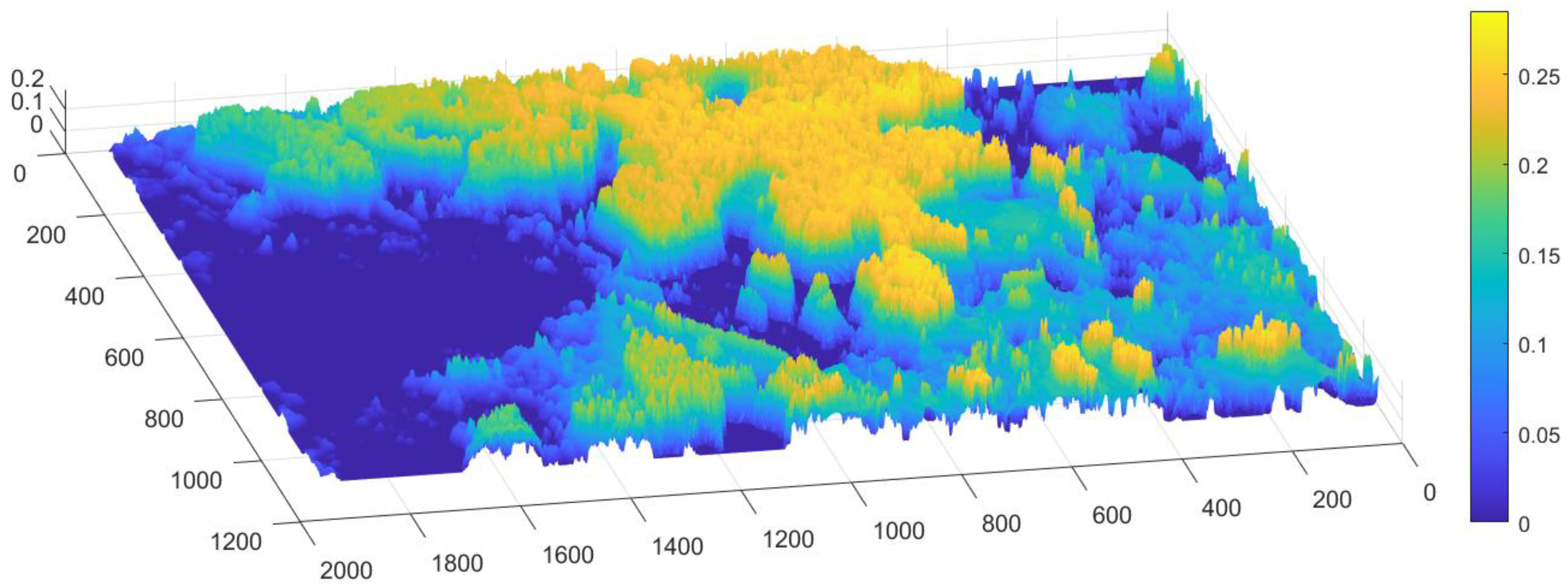
2.4. The Pseudo-3D Surface

An opaque mineral will undoubtedly be black in transmitted light because there is no way for light to pass through it. In polarized transmitted light, on the other hand, even non-opaque minerals show a certain intensity of reflected light on their own, but also due to internal reflections caused by anisotropy. These internal reflection effects are not present in a few cases, and the non-opaque mineral or the porosity is black in the reflected light. To overcome this reading difficulty in reflected light images and optimize the segmentation, we have implemented a method capable of simultaneously mapping minerals that exclusively transmit light and those that reflect it on the same surface. Among these, some reflect and partially transmit light. The method we have identified involves the construction of a three-dimensional surface whose z-axis provides information on which are the minerals that entirely transmit light, those that transmit/reflect it partially, and those that reflect it. To obtain a pseudo-3D surface (P3DS), we have added in addition to the two-dimensional information (x, y) a different z-axis which is the Euclidean distance between the intensity in a grayscale of the image acquired by reflected light and the one in transmitted light (Figure 4). In this way, when the CCD captures the light coming exclusively from an opaque mineral, the distance between the focal plane of the sample and the CCD detector will be shorter. Hence, the resulting difference will be equal to the intensity of the reflected light, and vice versa; if the light comes entirely from a non-opaque mineral, a long-distance beyond the focal plane of the reflected light will result and the Euclidean distance will be equivalent to the value of the intensity of the transmitted light, in shades of gray (Figure 5).

Following the diagram in Figure 4, the z-axis was obtained from the following Formula (2):

$$d=\sqrt{{\left(T_l-R_l\right)}^2}$$

(2)

where d is the Euclidean distance between the value (in shades of gray) of the transmitted light and the reflected light, T_l is the transmitted light, and R_l is the reflected light. The obtained values were then multiplied by the image metric scale calibration factor and used to determine the z-axis of the reconstructed pseudo-3D surface. In this way, the Euclidean distance d (a.u.) is reported in millimeters (mm).

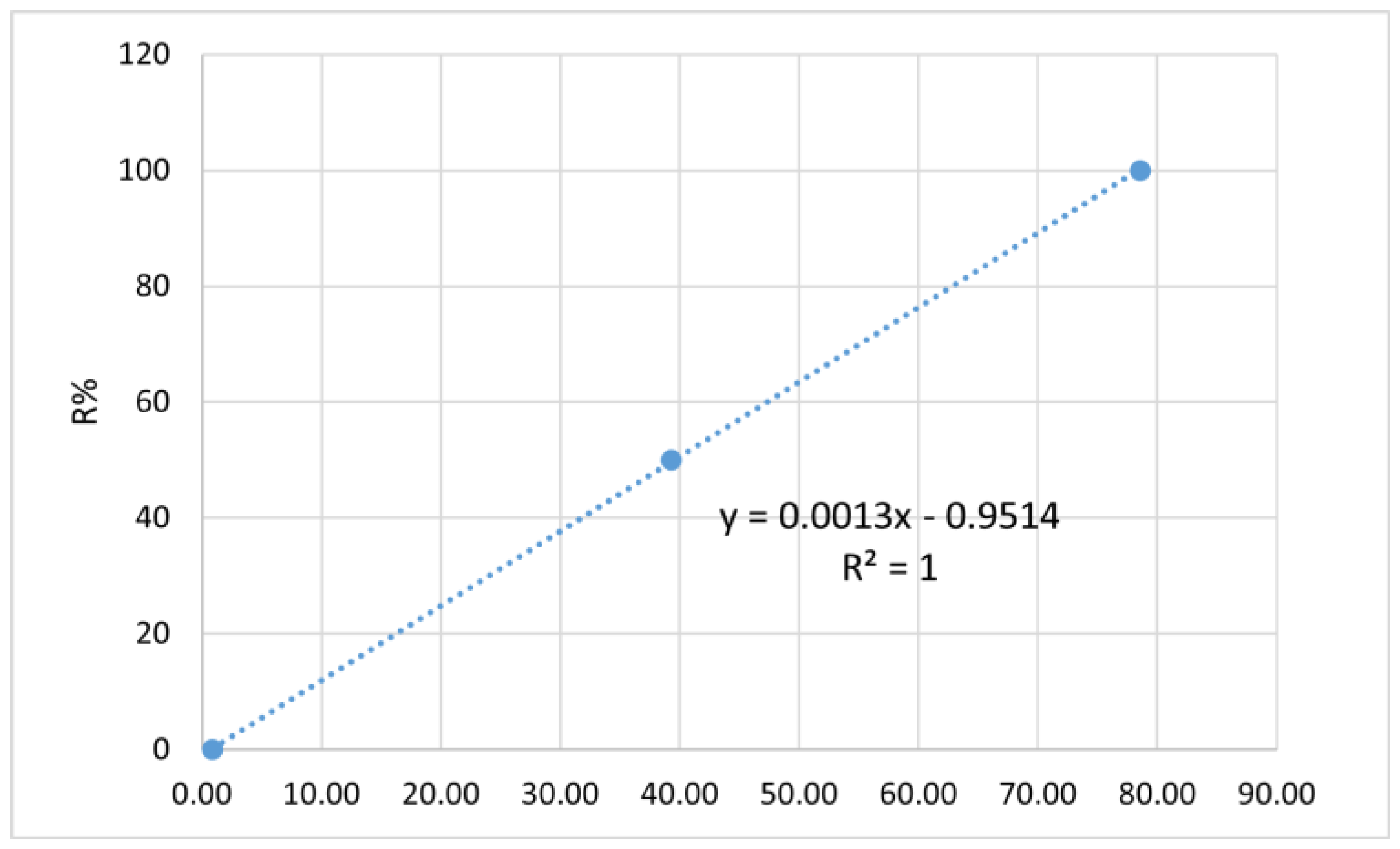
2.5. Calibration Curve and Reflectivity

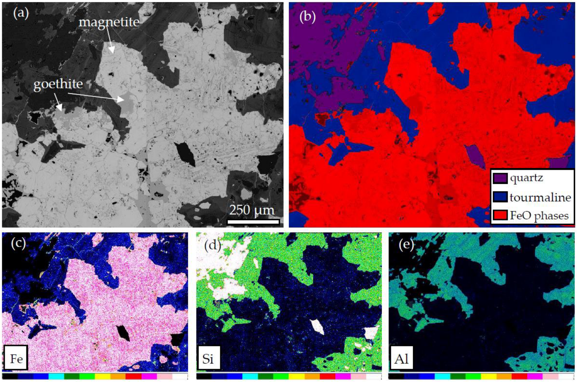
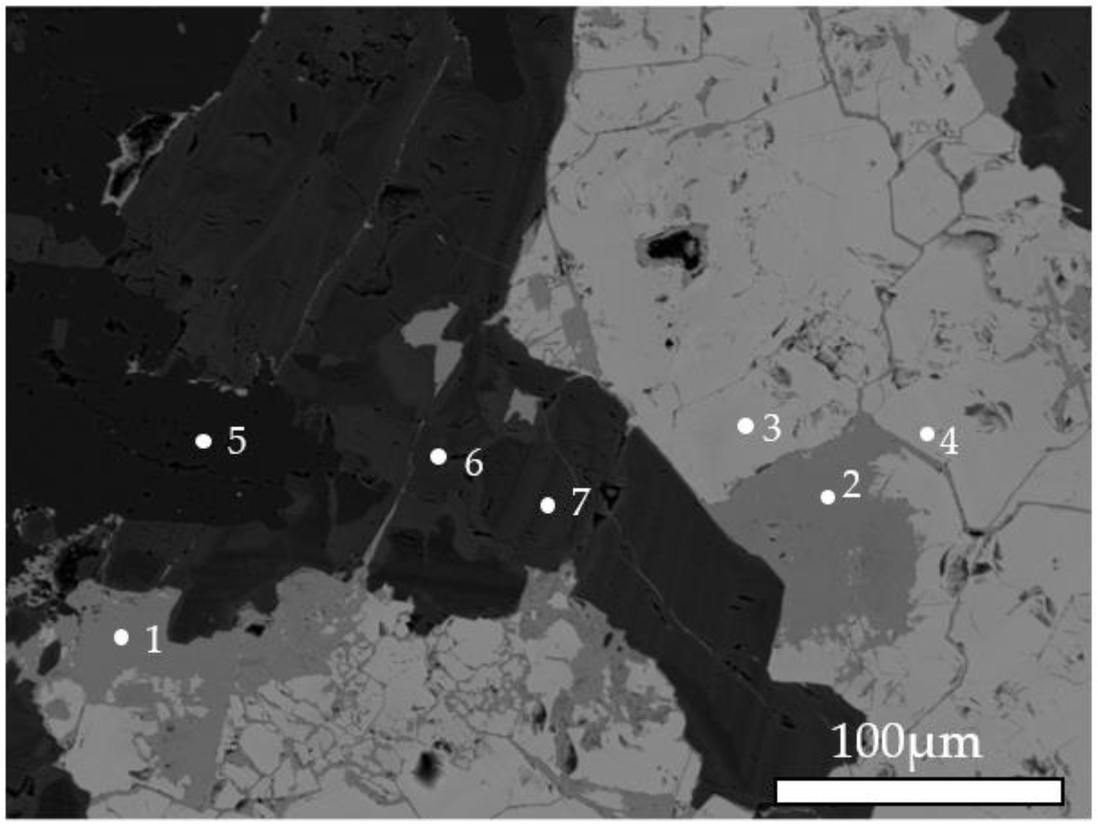
According to Craig et al. [19], the reflectivity (R%) is given by the ratio between the intensity of the reflected light at certain wavelength, multiplied by 100, and then divided by the intensity of the light incident on the sample (in our case, 100%) as in the following Equation (3).

$$\mathrm{R}\%=\frac{I_{Rl}·100}{I_{Il}}$$

(3)

where I_Rl was the intensity of the reflected light, and I_Il was the intensity of incident light.

The optical microscope we used is not equipped with a device for directly measuring the reflectivity of opaque minerals; hence, considering all the problems relating to the optical path, it was necessary to use an alternative method to obtain reliable results. Since we used the integral intensity of the luminance (a.u.) to measure the intensity of reflectivity, we substitute it in Formula (3) to obtain the reflectance values of the minerals present in the thin section.

Building a calibration curve based on three reference materials with reflectivity values (R%) of 100, 50, and 0, we assumed that the integral intensity of luminance in the color space L* a* b* was directly correlated to R% (Figure 6). The slope coefficients (0.0013) and the intercept (0.9514) of the calibration line were used to recalculate the R% value of each segment obtained from the SOM neural network. Finally, we compared the results with the original Craig et al. [19] Equation (3). We established the correlation between the R% value of analyzed minerals and their luminance (a.u.) integral intensity, and the correlation coefficient R² was equal to 1. Since the luminance value of an image is always affected by the individual luminance values within an image, we multiplied single pixels of each segment by its values of d and in our calibration curve before performing the calculations with the Craig et al. Equation (3), to mitigate this influence.

Given the generic equation of the line y = mx + q, we add a parameter k = d (Euclidean distance) which normalizes the luminance value to the only light reflected by the opaque minerals, discarding or attenuating the light transmitted by the semi-opaque or non-opaque minerals.

3. SEM Validation

SEM observation in backscattered electrons (SEM-BSE) on the area observed in optical microscopy, allowed the discrimination of goethite and magnetite minerals (bright grey in Figure 7a) and quartz and tourmaline (dark grey in Figure 7a). An autophase map was used to better discriminate the gangue phases by false color image (Figure 7b).

From the Fe map in Figure 7c, it is possible to observe the texture of the magnetite which is replaced by goethite along fractures and grain boundaries. A series of measurement points were carried out in a selected area to define the chemical composition of the mineralogical phases identified (Figure 8 and

Table 1. Concentration of major elements (SEM-EDS).

Element	Goethite		Magnetite		Quartz	Tourmaline
	Point 1	Point 2	Point 3	Point 4	Point 5	Point 6	Point 7
	wt%
O	25.82	26.07	29.24	29.45	53.3	34.91	35.17
Al	0.6	0.55	0.56			13.39	13.46
Na			0.16			1.3	1.18
Mg						4.31	5.27
Si	1.2	1.28	1.56	0.83	46.69	16.63	16.96
P	0.76	0.68
Ca	0.09		0.45	0.22		1.56	1.7
Ti						0.25	0.57
Fe	53.32	53.98	68.12	69.5		19.61	19.15
Sr		0.24
Total	81.78	82.8	100	100	99.99	91.95	93.46

).

4. Results and Discussion

The segmentation carried out with the SOM method allowed us to highlight the image’s characteristics quickly and quantify their percentage relative to the total area of the image. Figure 9 displays a pseudo-color image of the segmentation obtained using the SOM neural network. Through this first step, it was possible to estimate the percentage of area occupied by each segment regarding the analyzed image total area. Green and brown segments (respectively segments 1 and 2, Figure 10) represent only a tiny area of the image (16% green and 19% brown), while blue and cyan segments (respectively segments 3 and 4 in Figure 10) represents most of the image area (32% cyan and 34% blue). Segment 1 (green) refers to the opaque minerals (magnetite and goethite) present in the section. Segment 2 (brown) shows quartz minerals. Segment 3 (blue) shows the occurrence of tourmaline minerals. Finally, segment 4 (cyan) refers to mixed phases. At the used magnification scale, the neural network has not been able to resolve the different mineral features present, whether they are opaque, semi-opaque, or non-opaque. This issue is also since the information derived from the images acquired with a CCD camera (at any color space considered) (i.e., RGB, HSV, L* a* b*) are mutually influenced, and the only truly decorrelated information corresponds to those related to the mineral contact edges and textures present. Using different color spaces allowed us to segment well the areas where an opaque mineral is present from those where the opaque mineral is intergrown with a non-opaque mineral and those where only a non-opaque mineral is present. Other types of information should be added further to distinguish the different minerals present within these areas (e.g., information on the reflectance/absorbance spectrum). Although this may seem a severe limitation of the current method, this is not the case, as, for most industrial applications to whom our work is addressed, preliminary investigations only need broad information on the degree of release of the mineral from its gangue. Image analyses at higher magnification can be carried out to overcome this issue if needed.

At the used magnification scale, the analytical method applied was successful in clearly discriminating massive opaque minerals (magnetite and goethite) from gangue (quartz and tourmaline); a small portion of the areas (segment 4, 32%) displays the occurrence of opaque minerals disseminated in quartz or tourmaline.

The actual SOM segments are two-dimensional images that contain only logical values (0 and 1), which indicate the presence of a feature. Thus, starting from these images, it is possible to use image morphological operators to return information on the areas, diameters, perimeters, and axes of the minerals present in each segment. Once the number of classes of interest is established, an algorithm can extract these characteristics. For our purposes, we decided to report exclusively on the area of the size classes of minerals expressed in mm². The histograms of the segmented areas in Figure 10 show how most of the mineral grains areas are between 0.1 and 0.2 mm². Mineral grain sizes greater than 1.6 mm² are also present but occur with a mean lower frequency than the total mineral particulate < 1.6 mm². Segments 2 in Figure 10b, 3 in Figure 10c and 4 in Figure 10d refer to semi-opaque, non-opaque, or mixed occurrence of minerals. The SOM segmentation exclusively returns a reduction in the space of the incoming features, maintaining the same topologic information. From this, it is difficult to understand whether the segment we observe belongs to an opaque, semi-opaque, non-opaque mineral, or a mixture of these.

The P3DS (Figure 11) highlights the roughness characteristics in a 3D space. This 3D map was effective in distinguishing between opaque and non-opaque mineral phases. Moreover, P3DS allows appreciating even the minor details, which are commonly undetected or misidentified in a traditional 2D micro-photo. For instance, the presence of non-opaque minerals in tiny areas or spots of 2D image could be detected, and the opaque minerals can be well distinguished from the gangue groundmass (Figure 9). The P3DS represents an artificial construction that contains information about spatial topologies and the opaque/non-opaque nature of the mineral features represented. When observing the Euclidean distance (d) on the z-axis, it must be considered that the Z dimension is overestimated due to the different optical paths of the transmitted and reflected light. This overestimation is due to the thickness of the thin section slide. Opaque minerals will have greater distance (d > 0) values than semi-opaque and non-opaque minerals approaching d = 0. In the P3DS image of Figure 9, we observe a large portion of the two-dimensional space occupied by non-opaque minerals, representing our gangue (values of d ~ 0, in bluish color).

In contrast, the remaining portion of 2D space is occupied by opaque minerals (values of d ~ 0.2, in ochre-yellowish color), which are the ores, and by opaque minerals intergrown with non-opaque gangue or a mixture of these two phases (values of d ~ 0.1, in greenish color). The opaque minerals scattered in the gangue, are present as isolated spikes on the 3D surface or grouped in modest masses that emerge from the background and stand up in reliefs that gently fade towards the bottom gangue. If we look at the edge of an area of opaque minerals and compare it to areas with intermediate values of d (approximately between 0.1 and 0.15, in greenish color), we can observe that these are probably generated by opaque minerals finely intergrown with a non-opaque mineral. It is essential to highlight that this level is not clear in the SOM segmentation, but the modal estimation of the grain sizes is statistically representative of the sizes of the mineral present.

The contact borders between the different mineral species appear slopes-like due to the edge effect that attenuates the reflectance in the transition between an opaque and a non-opaque mineral; the greater the difference in reflectance between the observed materials is, the more this effect is accentuated [59,60]. This effect is difficult to evaluate on a two-dimensional image, while it is clear and evident in 3D surface representation.

Table 2. Values of reflectivity (R%) in air obtained after correction by the mean of the Euclidean distance d.

Segments	R% in Air with Craig et al. [19] Equation (3)	R% in Air with Our Calibration
seg 1	13.9	15.2
seg 2	0.4	1.4
seg 3	10.1	11.3
seg 4	0.9	1.9

displays the values of reflectivity (R%) in air. The calculation of R% was obtained after correction with the Euclidean distance values (d) between the luminance of the micro-photo in RLM and TLM.

The results show that segment 1, referring to opaque minerals, has the highest R% value. Segment 3, which includes mixing situations between opaque, semi-opaque, and non-opaque minerals, has a slightly lower R% than segment 1. On the contrary, segments 2 and 3, referring to non-opaque minerals, show the lowest values of R%, very close to 0. This method allows the operator to bypass the particulate de-agglomeration procedure before carrying out the analysis, which would typically require a grinding step, X-ray powder diffraction, and SEM-EDS on particulate to discriminate and identify the relevant mineral phases from the gangue. Furthermore, considering the statistical data obtained from the segmentation, we can quickly understand that segment 3 must also be considered in calculating the area occupied by metal ores, even if intergrown with non-opaque gangue minerals.

The values shown in Table 2 must be considered relatively as for two factors: (i) we are considering a case in which the incident light is not monochromatic; (ii) there are several attenuation factors of the light reflected from the sample that we are not considering within our method. Nevertheless, by building a set of reference standards using monochromatic light and building a calibration curve for the optical path from the lamp to the sample and from the sample to the detection system, these numbers can be reported to values closer to those of reference for opaque minerals [19]. The determination of the area and grain size of valuable minerals serves as a guide for the grinding processes of the bulk rock. Being aware that most of the valuable minerals fall within a specific size, we can address the choice of grinding the rock to that size, hence increasing the degree of liberation of the ores using quick and inexpensive analysis. In the three areas where opaque minerals trapped by gangue minerals occur, we observe that the size distribution falls mostly between 0.3 and 1.1 mm, with a slightly higher frequency between 0.3 and 0.4 mm. Hence, to obtain the maximum degree of liberation of the valuable minerals from the gangue, grinding the rock below 0.4 mm will be sufficient. The identification and quantification of mixed gangue phases, yet at first preliminary observation in thin section, can immediately help to identify a likely loss of economically exploitable minerals destined to accumulate within tailings and determine, in the first instance, optimization of the processing strategies that do not involve further treatment of the waste materials, with considerable economic advantages. Indeed, the methods of AM allow obtaining more precise analysis, providing the mineralogy and chemistry of the minerals present and the degree of liberation. However, these systems have very high analytical costs, which small companies can hardly afford. Additionally, in some cases, expensive AM methods might sometimes be unnecessary due to the low complexity of the deposit mineralogy.

Although information on the potential liberation of the ores is still essential. Hence, using RLM as a quick and cheap method might still represent a significant advantage to better address the processing route and benefit further industrial operation.

5. Conclusions and Recommendations

Thanks to the new and increasingly refined image analysis methods, optical microscopy is still a valid methodology for analyzing ore minerals. These methods allow, with good approximations, to model various fundamental parameters for Mineral Liberation Analysis (MLA), which is fundamental in mining and metallurgical applications. Using simple algorithms of Image Analyses and application of neural networks, we can approximate a calculation of the area occupied by valuable ore minerals in respect to gangue. We can establish the grain size distribution for opaque and non-opaque minerals, although some errors due to the automatic determination algorithm must be considered. These errors arise because the definition of the edge of the grains and their interior, being a heuristic process based on the operator’s experience, can suffer from a certain degree of uncertainty. Without conducting preliminary grinding of the sample, we can determine directly from the thin section at which size we should grind the sample to obtain an optimal liberation of ore minerals.

We are aware that the resolution obtained by an optical microscope is very different from that possible with an SEM, which affects our measurement results. However, in this work, we have presented a fast and low-cost tool for a preliminary evaluation and immediate identification of some fundamental parameters to consider while studying ore minerals for mining industry applications.

Additional Comments

This work is a preliminary study that refers to the first three levels of the technology readiness level (TRL1–3) and constitutes an experimental proof of concept (TRL3) that requires further tests to improve and validate the methodology; laboratory tests (TRL4) and application to industry (TRL5) will be further planned and carried out. Additional considerations on the hardware and the algorithms used and tested can be made based on the results of the tests.

Future work would be to use higher-magnification objectives on a microscope capable of mapping areas to obtain more accurate results although the resolution of the optical microscope can never be smaller than the diffraction limit of light, even using adaptive lenses. Perhaps the future the development of new generation lenses made of metamaterials will allow us to go beyond this physical limit. For more precise and accurate results, we would like to be able to exploit higher-magnification objectives on a microscope capable of mapping areas.

References

1. Clarke, A.; Eberhardt, C.; Eberhardt, C.N. Microscopy Techniques for Materials Science; Woodhead Publishing: Boca Raton, FL, USA, 2002. [Google Scholar]
2. Hrstka, T.; Gottlieb, P.; Skala, R.; Breiter, K.; Motl, D. Automated mineralogy and petrology-applications of TESCAN Integrated Mineral Analyzer (TIMA). J. Geosci. 2018, 63, 47–63. [Google Scholar] [CrossRef] [Green Version]
3. Maloy, A.K.; Treiman, A.H. Evaluation of image classification routines for determining modal mineralogy of rocks from X-ray maps. Am. Mineral. 2007, 92, 1781–1788. [Google Scholar] [CrossRef]
4. Schulz, B.; Sandmann, D.; Gilbricht, S. SEM-based automated mineralogy and its application in geo-and material sciences. Minerals 2020, 10, 1004. [Google Scholar] [CrossRef]
5. Schofield, P.F.; Knight, K.S.; Covey-Crump, S.J.; Cressey, G.; Stretton, I.C. Accurate quantification of the modal mineralogy of rocks when image analysis is difficult. Mineral. Mag. 2002, 66, 189–200. [Google Scholar] [CrossRef]
6. McSween, H.Y., Jr.; McGlynn, I.O.; Rogers, A.D. Determining the modal mineralogy of Martian soils. J. Geophys. Res. Planets 2010, 115, E00F12. [Google Scholar] [CrossRef] [Green Version]
7. Koch, P.-H.; Lund, C.; Rosenkranz, J. Automated drill core mineralogical characterization method for texture classification and modal mineralogy estimation for geometallurgy. Miner. Eng. 2019, 136, 99–109. [Google Scholar] [CrossRef]
8. Koh, E.J.Y.; Amini, E.; McLachlan, G.J.; Beaton, N. Utilising convolutional neural networks to perform fast automated modal mineralogy analysis for thin-section optical microscopy. Miner. Eng. 2021, 173, 107230. [Google Scholar] [CrossRef]
9. Hoal, K.O.; Stammer, J.G.; Appleby, S.K.; Botha, J.; Ross, J.K.; Botha, P.W. Research in quantitative mineralogy: Examples from diverse applications. Miner. Eng. 2009, 22, 402–408. [Google Scholar] [CrossRef]
10. Sorby, H.C. XII. On the microscopical structure of meteorites. Proc. R. Soc. Lond. 1864, 13, 333–334. [Google Scholar]
11. Hammond, C. The contribution of Henry Clifton Sorby to the study of reflected light microscopy of iron and steel. Hist. Metall. 1989, 23, 1–8. [Google Scholar]
12. Hardwick, D.A.; Williams, W.M. The birth of metallography- The work of Henry Clifton Sorby (1826–1908). Bull. Can. Inst. Min. Metall. 1980, 73, 143–144. [Google Scholar]
13. Perrin, L. Henry Clifton Sorby and the Beginnings of Microscopial Metallography. Doctoral Dissertation, Oxford University, Oxford, UK, 1976. [Google Scholar]
14. Ramdohr, P. The Ore Minerals and Their Intergrowths; Elsevier Ltd.: Oxford, UK, 2013. [Google Scholar]
15. Chryssoulis, S.L.; McMullen, J. Mineralogical investigation of gold ores. Dev. Miner. Process. 2005, 15, 21–71. [Google Scholar]
16. Piller, H. Colour measurements in ore-microscopy. Miner. Depos. 1966, 1, 175–192. [Google Scholar] [CrossRef]
17. Ineson, P.R. Introduction to Practical Ore Microscopy; Routledge, Taylor & Francis Group: London, UK; New York, NY, USA, 2014. [Google Scholar]
18. Bowie, S.H.U.; Taylor, K. A System of Ore Mineral Identification; Geological Survey: London, UK, 1959. [Google Scholar]
19. Craig, J.R.; Vaughan, D.J.; Hagni, R.D. Ore Microscopy and Ore Petrography; Wiley: New York, NY, USA, 1981. [Google Scholar]
20. Uytenbogaardt, W.; Burke, E.A.J. Tables for Microscopic Identification of Ore Minerals; Courier Corporation: New York, NY, USA, 1985. [Google Scholar]
21. Sánchez-Ramos, S.; Doménech-Carbó, A.; Gimeno-Adelantado, J.V.; Peris-Vicente, J. Analytical and mineralogical studies of ore and impurities from a chromite mineral using X-ray analysis, electrochemical and microscopy techniques. Talanta 2008, 74, 1592–1597. [Google Scholar] [CrossRef]
22. Kahn, H.; Mano, E.S.; Tassinari, M. Image analysis coupled with a SEM-EDS applied to the characterization of a partially weathered Zn-Pb ore. J. Miner. Mater. Charact. Eng. 2002, 1, 1–9. [Google Scholar]
23. Donskoi, E.; Manuel, J.R.; Austin, P.; Poliakov, A.; Peterson, M.J.; Hapugoda, S. Comparative study of iron ore characterisation using a scanning electron microscope and optical image analysis. Appl. Earth Sci. 2013, 122, 217–229. [Google Scholar] [CrossRef]
24. Reyes, F.; Lin, Q.; Udoudo, O.; Dodds, C.; Lee, P.D.; Neethling, S.J. Calibrated X-ray micro-tomography for mineral ore quantification. Miner. Eng. 2017, 110, 122–130. [Google Scholar] [CrossRef] [Green Version]
25. Mohanan, S.; Bhoja, S.K.; Kumar, C.R.; Kumar, A.; Venugopalan, T. Estimation of ore mineralogy from analytical analysis of iron ore. Min. Metall. Explor. 2015, 32, 97–101. [Google Scholar] [CrossRef]
26. Gu, Y. Automated scanning electron microscope based mineral liberation analysis an introduction to JKMRC/FEI mineral liberation analyser. J. Miner. Mater. Charact. Eng. 2003, 2, 33–41. [Google Scholar] [CrossRef]
27. Fandrich, R.; Gu, Y.; Burrows, D.; Moeller, K. Modern SEM-based mineral liberation analysis. Int. J. Miner. Process. 2007, 84, 310–320. [Google Scholar] [CrossRef]
28. Gottlieb, P.; Wilkie, G.; Sutherland, D.; Ho-Tun, E.; Suthers, S.; Perera, K.; Jenkins, B.; Spencer, S.; Butcher, A.; Rayner, J. Using quantitative electron microscopy for process mineralogy applications. JOM 2000, 52, 24–25. [Google Scholar] [CrossRef]
29. Pirrie, D.; Butcher, A.R.; Power, M.R.; Gottlieb, P.; Miller, G.L. Rapid quantitative mineral and phase analysis using automated scanning electron microscopy (QemSCAN); potential applications in forensic geoscience. Geol. Soc. Lond. Spec. Publ. 2004, 232, 123–136. [Google Scholar] [CrossRef]
30. Graham, S.D.; Brough, C.; Cropp, A. An introduction to ZEISS mineralogic mining and the correlation of light microscopy with automated mineralogy: A case study using BMS and PGM analysis of samples from a PGE-bearing chromite prospect. In Proceedings of the Precious Metals’15, Falmouth, UK, 13–14 May 2015; pp. 1–12. [Google Scholar]
31. Ayling, B.; Rose, P.; Petty, S.; Zemach, E.; Drakos, P. QEMSCAN (Quantitative evaluation of minerals by scanning electron microscopy): Capability and application to fracture characterization in geothermal systems. In Proceedings of the Thirty-Seventh Workshop on Geothermal Reservoir Engineering, Stanford, CA, USA, 30 January–1 February 2012. [Google Scholar]
32. Andersen, J.C.Ø.; Rollinson, G.K.; Snook, B.; Herrington, R.; Fairhurst, R.J. Use of QEMSCAN® for the characterization of Ni-rich and Ni-poor goethite in laterite ores. Miner. Eng. 2009, 22, 1119–1129. [Google Scholar] [CrossRef]
33. Donskoi, E.; Manuel, J.; Austin, P.; Poliakov, A.; Peterson, M.; Hapugoda, S. Comparative study of iron ore characterisation by optical image analysis and QEMSCAN (TM). In Proceedings of the Iron Ore 2011, Perth, WA, Australia, 11–13 July 2011. [Google Scholar]
34. Gu, Y.; Schouwstra, R.P.; Rule, C. The value of automated mineralogy. Miner. Eng. 2014, 58, 100–103. [Google Scholar] [CrossRef]
35. Harmon, R.S.; Lawley, C.J.M.; Watts, J.; Harraden, C.L.; Somers, A.M.; Hark, R.R. Laser-induced breakdown spectroscopy—An emerging analytical tool for mineral exploration. Minerals 2019, 9, 718. [Google Scholar] [CrossRef]
36. Nikonow, W.; Rammlmair, D.; Meima, J.A.; Schodlok, M.C. Advanced mineral characterization and petrographic analysis by μ-EDXRF, LIBS, HSI and hyperspectral data merging. Mineral. Petrol. 2019, 113, 417–431. [Google Scholar] [CrossRef]
37. Lawley, C.J.M.; Somers, A.M.; Kjarsgaard, B.A. Rapid geochemical imaging of rocks and minerals with handheld laser induced breakdown spectroscopy (LIBS). J. Geochem. Explor. 2021, 222, 106694. [Google Scholar] [CrossRef]
38. El Haddad, J.; de Lima Filho, E.S.; Vanier, F.; Harhira, A.; Padioleau, C.; Sabsabi, M.; Wilkie, G.; Blouin, A. Multiphase mineral identification and quantification by laser-induced breakdown spectroscopy. Miner. Eng. 2019, 134, 281–290. [Google Scholar] [CrossRef]
39. Senesi, G.S.; Capitelli, F. Compositional, mineralogical and structural investigation of meteorites by XRD and LIBS. In Hypersonic Meteoroid Entry Physics; IOP Publishing: Bristol, UK, 2019. [Google Scholar] [CrossRef]
40. Haavisto, O.; Kauppinen, T.; Häkkänen, H. Laser-induced breakdown spectroscopy for rapid elemental analysis of drillcore. IFAC Proc. Vol. 2013, 46, 87–91. [Google Scholar] [CrossRef]
41. Mohamed, N.; Rifai, K.; Selmani, S.; Constantin, M.; Doucet, F.R.; Özcan, L.Ç.; Sabsabi, M.; Vidal, F. Chemical and Mineralogical Mapping of Platinum-Group Element Ore Samples Using Laser-Induced Breakdown Spectroscopy and Micro-X-ray Fluorescence. Geostand. Geoanal. Res. 2021, 45, 539–550. [Google Scholar] [CrossRef]
42. Paradis, M.-C.M.; Doucet, F.R.; Rifai, K.; Özcan, L.Ç.; Azami, N.; Vidal, F. ECORE: A new fast automated quantitative mineral and elemental core scanner. Minerals 2021, 11, 859. [Google Scholar] [CrossRef]
43. Rifai, K.; Michaud Paradis, M.-C.; Swierczek, Z.; Doucet, F.; Özcan, L.; Fayad, A.; Li, J.; Vidal, F. Emergences of new technology for ultrafast automated mineral phase identification and quantitative analysis using the CORIOSITY Laser-Induced Breakdown Spectroscopy (LIBS) system. Minerals 2020, 10, 918. [Google Scholar] [CrossRef]
44. Ross, L.; Russ, J.C. The image processing handbook. Microsc. Microanal. 2011, 17, 843. [Google Scholar] [CrossRef]
45. Kohonen, T. The self-organizing map. Neurocomputing 1998, 21, 1–6. [Google Scholar] [CrossRef]
46. Kohonen, T. Self-Organization and Associative Memory; Springer Science & Business Media: Berlin/Heidelberg, Germany, 2012. [Google Scholar]
47. Kohonen, T. The self-organizing map. Proc. IEEE 1990, 78, 1464–1480. [Google Scholar] [CrossRef]
48. Jiang, D.; Yang, Y.; Xia, M. Research on intrusion detection based on an improved SOM neural network. In Proceedings of the 2009 Fifth International Conference on Information Assurance and Security, Xi’an, China, 18–20 August 2009; pp. 400–403. [Google Scholar]
49. Chen, L.-P.; Liu, Y.-G.; Huang, Z.-X.; Shi, Y.-T. An improved SOM algorithm and its application to color feature extraction. Neural Comput. Appl. 2014, 24, 1759–1770. [Google Scholar] [CrossRef] [Green Version]
50. Smits, J.R.M.; Melssen, W.J.; Buydens, L.M.C.; Kateman, G. Using artificial neural networks for solving chemical problems: Part I. Multi-layer feed-forward networks. Chemom. Intell. Lab. Syst. 1994, 22, 165–189. [Google Scholar] [CrossRef] [Green Version]
51. Livingstone, D.J. Artificial Neural Networks: Methods and Applications; Springer: Totowa, NJ, USA, 2008. [Google Scholar]
52. Zupan, J. Introduction to artificial neural network (ANN) methods: What they are and how to use them. Acta Chim. Slov. 1994, 41, 327. [Google Scholar]
53. Ng, H.P.; Ong, S.H.; Foong, K.W.C.; Goh, P.S.; Nowinski, W.L. Medical image segmentation using k-means clustering and improved watershed algorithm. In Proceedings of the 2006 IEEE Southwest Symposium on Image Analysis and Interpretation, Denver, CO, USA, 26–28 March 2006; pp. 61–65. [Google Scholar]
54. Akinin, M.V.; Taganov, A.I.; Nikiforov, M.B.; Sokolova, A.V. Image segmentation algorithm based on self-organized Kohonen’s neural maps and tree pyramidal segmenter. In Proceedings of the 2015 4th Mediterranean Conference on Embedded Computing (MECO), Budva, Montenegro, 14–18 June 2015; pp. 168–170. [Google Scholar]
55. Lee, Y.-K.; Rhodes, W.T. Nonlinear image processing by a rotating kernel transformation. Opt. Lett. 1990, 15, 1383–1385. [Google Scholar] [CrossRef]
56. Thum, C. Measurement of the entropy of an image with application to image focusing. Opt. Acta Int. J. Opt. 1984, 31, 203–211. [Google Scholar] [CrossRef]
57. Chang, D.-C.; Wu, W.-R. Image contrast enhancement based on a histogram transformation of local standard deviation. IEEE Trans. Med. Imaging 1998, 17, 518–531. [Google Scholar] [CrossRef] [PubMed] [Green Version]
58. Ranganath, A.; Senapati, M.R.; Sahu, P.K. Estimating the fractal dimension of images using pixel range calculation technique. Vis. Comput. 2021, 37, 635–650. [Google Scholar] [CrossRef]
59. Wood, B.J.; Strens, R.G.J. Diffuse reflectance spectra and optical properties of some sulphides and related minerals. Mineral. Mag. 1979, 43, 509–518. [Google Scholar] [CrossRef] [Green Version]
60. Poliakov, A.; Donskoi, E. Automated relief-based discrimination of non-opaque minerals in optical image analysis. Miner. Eng. 2014, 55, 111–124. [Google Scholar] [CrossRef]
Figure 1. Micro-photo of the thin section of the selected rock section: (a) reflected light; (b) transmitted light with crossed Nicols. The long side of the image measures 2.7 mm, and each micro-photo has the same scale.
Minerals 12 01348 g001
Figure 2. The filtered micro-photo both reflected and transmitted light. Entropy (a), standard deviation (b), and range (c) represent filtering of reflected light micro-photo. Entropy (d), standard deviation (e), and range (f) represent filtering of transmitted light micro-photo. The long side of the image is 2.7 mm.
Minerals 12 01348 g002
Figure 3. The images derived from filtering with a 3 × 3 pixel kernel whose value of the central pixel is 127.5, while the contour pixels all have a value of 0. On the left (a) is the result of the convolution with the image in reflected light, while on the right (b), we observe the result obtained on the transmitted light.
Minerals 12 01348 g003
Figure 4. Conceptual scheme of z-axis calculation for pseudo-surface.
Minerals 12 01348 g004
Figure 5. Mapping of each pixel’s Euclidean distance between reflected and transmitted light. Brighter pixels indicate opaque minerals, while less bright pixels indicate non-opaque or partially opaque minerals. Situations, where non-opaque minerals cover opaque minerals (they show a dimmed brightness) are noticeable.
Minerals 12 01348 g005
Figure 6. Calibration curve of reflectivity (R%).
Minerals 12 01348 g006
Figure 7. SEM maps of the selected area. (a) BSE montage map (4 frames 70×); (b) phase map in false color; (c) quantitative EDS map of Fe; (d) quantitative EDS map of Si; (e) quantitative EDS map of Al (same area but the images are all upside down).
Minerals 12 01348 g007
Figure 8. Position of the EDS analysis points in the selected area.
Minerals 12 01348 g008
Figure 9. SOM segmentation image (a): cyan = 32% (mixed phases); brown = 19% (quartz); blue = 34% (tourmaline); green = 16% (magnetite and goethite). Reflected light image (b) for comparation. Long side is 2.7 mm.
Minerals 12 01348 g009
Figure 10. Segmented areas and their histograms from the grain size distribution algorithm. (a) Seg 1 Eq. Area (mm2); (b) Seg 2 Eq. Area (mm2); (c) Seg 3 Eq. Area (mm2); (d) Seg 4 Eq. Area (mm2).
Minerals 12 01348 g010
Figure 11. Pseudo-3D surface of the sample (P3DS). It shows the micro morphology of the surface. Taking in accounts the non-homogeneous point by point homogeneity of the reflected light from the sample it shows some interesting features. The color bar represents the Euclidean distance (d) expressed in mm; on the x and y axes, there are pixel numbers. The 3D reconstruction is specular to the original image. The x and y axes are in pixels.
Minerals 12 01348 g011