On the Modeling of Energy-Multisource Networks by the Thermostatted Kinetic Theory Approach: A Review with Research Perspectives

Abstract

Recently, different mathematical frameworks of the thermostatted kinetic theory approach have been proposed for the modeling of complex systems. In particular, thermostatted kinetic frameworks have been employed for the modeling and time evolution of a hybrid energy-multisource network composed of renewable and nonrenewable energy sources, for the construction of the energy storage and for open networks. In the frameworks of the thermostatted kinetic theory approach, the evolution of an energy source and the interactions with other energy sources are modeled by introducing a distribution function and interaction rates. This paper is a survey of the recent proposed frameworks of the thermostatted kinetic theory for the modeling of a hybrid energy-multisource network and reviews the recent proposed models. The paper is not limited to review the existing frameworks, but it also generalizes the mathematical structures proposed in the pertinent literature and outlines future research perspectives and applications of this new approach proposed in 2012.

1. Introduction

Since the last century, the need for energy has been increasing [1,2]. On the other hand, the attention and the impact to climate change have been increasing as well. Consequently, the development of new sources of renewable energy and the definition of smart energy source networks have gained a lot of attention. Environmental, technological but also economical issues are at the base of an optimal smart power grid. The modeling of a smart power grid is thus part of the class of the complex systems; see, among others, [3,4,5]. The reader interested in the general theory of the complex systems is referred to [6,7,8]. Accordingly, the modeling of a smart power grid shares many characteristics with the complex systems and in particular the important role of the exchange of information and the interactions [9,10].

This paper focuses on the modeling of hybrid networks of energy-multisources. According to the hybrid multisource network definition, nonrenewable and renewable energy sources are settled into a geographic area possibly divided into different regions; the national distribution network and storage systems are usually part of the hybrid network [11,12]. As already mentioned, renewable energy sources are also part of hybrid networks, and these sources of energy account nowadays for the major part of the total consumption [13]. As is known, geothermal energy, planetary energy and solar energy are the most important renewable energies. Specifically, geothermal energy is based on the heat stored in the earth [14]; the planetary energy takes advantage of the forces acting on the surface of the earth as a consequence of the movement of the celestial bodies [15]; the direct solar energy is originated by the solar radiation (e.g., thermodynamic, thermal and photovoltaic) and the indirect solar energy [16], e.g., wind turbine, biomass.

The planning and the optimization of hybrid energy-multisource networks are a fruitful research domain, which has been characterized by the interactions of different scholars coming from the different applied sciences. Different approaches have been proposed and employed in an attempt to construct a robust theory. The sizing of the hybrid multisource networks is not an easy task, and the appeal to optimization methods is a required step [17,18,19,20,21]. The stochastic role of the networks has also been taken into account by employing methods based on probability; see [22,23,24,25]. Approaches based on the artificial intelligence have also been proposed; see papers [26,27,28,29] and the reference cited therein. Differential equations-based models have also been derived [30,31,32,33], along with Petri Net frameworks [34] and topological structures [35,36]. Recent contributions can be found in [37,38] and the reference section. The reader is referred to [2,39] for a deeper critical analysis on the existing models.

This paper is a review of the recently proposed thermostatted kinetic theory approach and related models for the development and analysis of hybrid multisource networks. The thermostatted kinetic theory has been proposed in 2012 for the modeling of complex living systems and in particular for nonequilibrium adaptive complex systems [40]. According to the thermostatted kinetic theory approach, the system is composed of a large number of active particles, which are able to interact with each other and develop specific functions and strategies. In particular, the theory is based on a system theory approach where the active particles are grouped into subsystems constituted by particles expressing the same function (functional subsystems) [41]. The microscopic state of the particles is composed of space and velocity variables, and the function expressed by the particles is taken into account by introducing into the microscopic state of the particles a scalar/vectorial variable called activity; see the recent paper [42]. The evolution of the system thus corresponds to the time evolution and interaction of each functional subsystem, which are described by introducing a distribution function defined over the microscopic state of the particles. The evolution equation system fulfilled by the distribution functions is obtained by considering the inlet and outlet flows based on the interactions. In particular, two kinds of interactions have been defined: conservative interactions that model the changing into the value of the microscopic variables and nonconservative interactions which modify the magnitude of the macroscopic variables (e.g., the density of the system). The interactions are usually modeled by stochastic terms based on jump-processes [43] and game theory [44]. As already mentioned, the system under consideration is usually out-of-equilibrium, namely subjected to a macroscopic external force field coupled to a thermostat term in order to ensure the existence of nonequilibrium stationary states [45,46,47]. It is worth stressing that the microscopic activity variable can attain discrete or continuous values and consequently the equation of the model can be ordinary or partial differential equations. Hybrid equations have also been proposed where some microscopic variables are defined in a discrete domain, and the other microscopic variables are defined in a continuous domain [48]. Bearing all of the above in mind, the thermostatted kinetic theory takes advantage of different approaches and specifically of kinetic theory [49,50], nonequilibrium statistical mechanics [51], information theory [52], inverse theory [53] and game theory. From the application point of view, models of the thermostatted kinetic theory have been proposed for the modeling of the immune system [54], cancer-immune system competition [55], keloid formation and therapy [56], for the modeling of pedestrian dynamics [57], financial systems [58] and recently for the modeling of smart grids [59,60,61,62].

As already mentioned, the present paper is devoted to the thermostatted kinetic theory frameworks proposed for the modeling of hybrid networks composed of both nonrenewable energy sources and renewable energy sources. The interactions with external networks and the construction of the energy storage systems are also taken into account. The main aim of these frameworks is the possibility to develop specific models for studying the possibility to improve the quality of the energy provided to the customers and thus promoting the activation of the renewable energy source with respect to the nonrenewable energy source. The paper is not only a review considering that generalization of previous frameworks is proposed with the aim of constructing a robust and general theory, and perspectives of research and future research directions are also mentioned in the whole paper. However, the review part is rather in the description of the specific models that have been derived and proposed in the literature.

The present review paper is organized into six more sections, which follow this introduction. In particular, the paper is divided into two parts: In the first part (Section 2, Section 3 and Section 4), the mathematical frameworks of the thermostatted kinetic theory are reviewed while, in the second part (Section 5 and Section 6), the specific models proposed in the pertinent literature are presented, and the results of the computational analysis are briefly mentioned.

In detail:

-

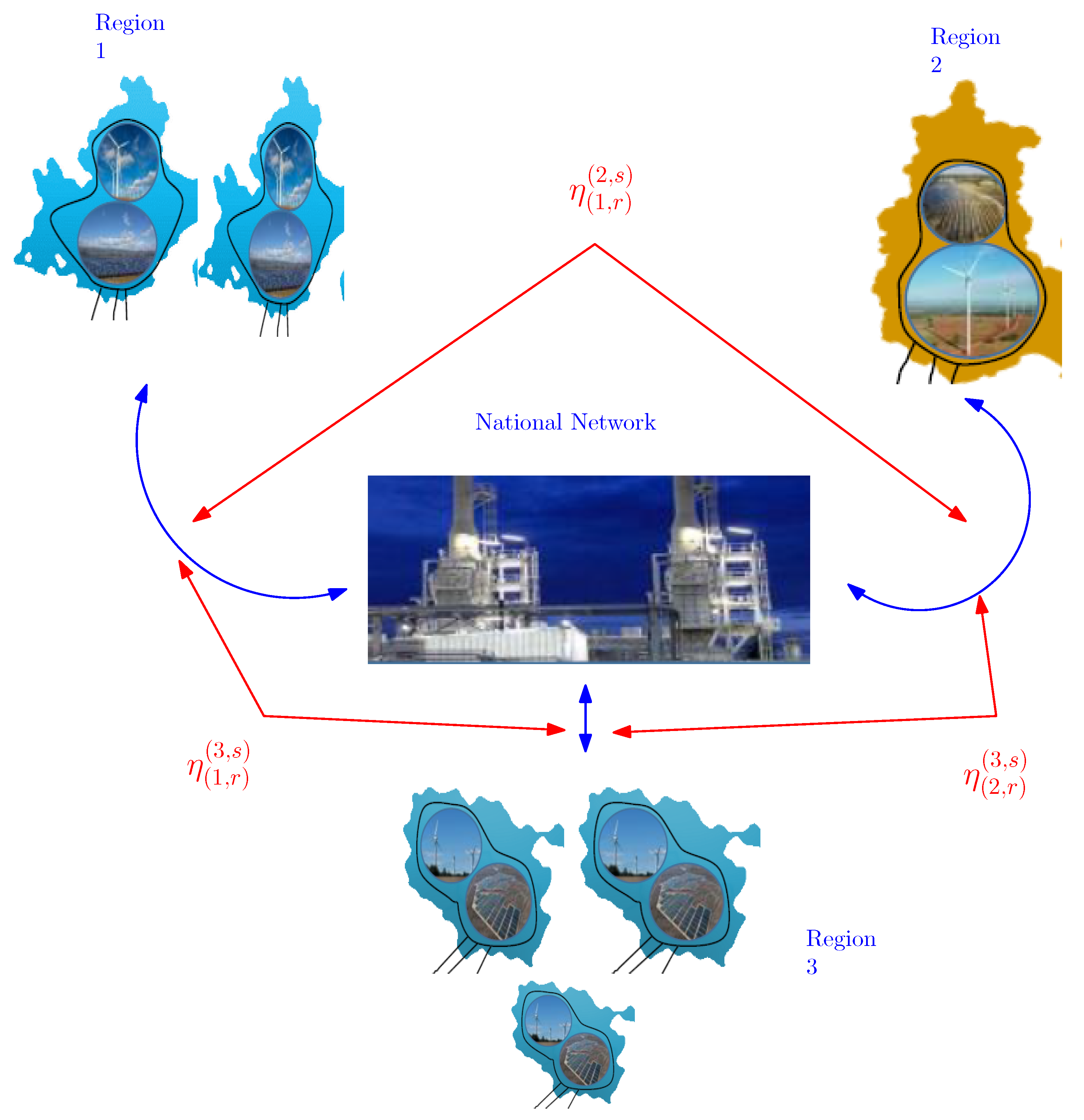
Section 2 summarizes, at a tutorial level, the main ingredients of the thermostatted kinetic theory framework recently proposed for the modeling of a closed network composed of multisources of energy allocated into different regions of a geographical area. The mathematical results and the pertinent literature are also mentioned. It is worth stressing that the section is not limited to the review of the existing thermostatted kinetic theory framework, but the thermostatted framework proposed in this section is further generalized considering that the number of sources allocated in each region is not required to be the same as proposed in [59]. The material of this section is thus original.

-

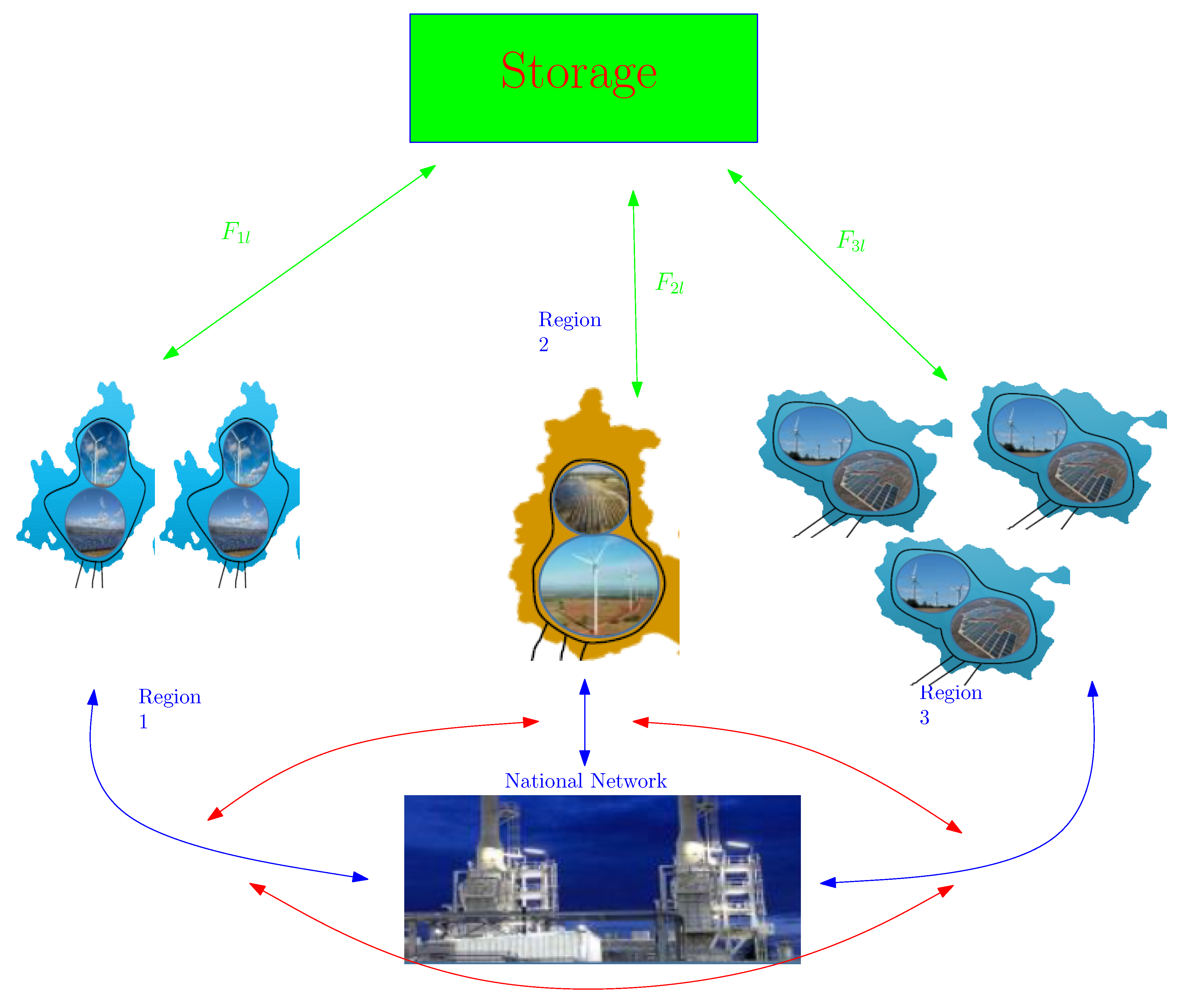
Section 3 introduces the problem of the modeling of the energy storage system. Specifically, the section reviews, under the previously mentioned generalization, the introduction of the energy storage in the thermostatted kinetic theory framework by introducing an external force field whose magnitude is responsible for the construction of the energy storage. In particular, and differently from the framework proposed in Section 2, the framework proposed in Section 3 is a pure thermostatted framework considering that the action of the external force field is balanced by the introduction of a damping term, called the thermostat operator, which allows for the reaching of a nonequilibrium stationary state.

-

Section 4 deals with open networks of energy sources. Specifically, the thermostatted frameworks proposed in the previous sections are generalized to introduce the interaction of the network with external networks (regional or national). Moreover, the framework proposed in this section can be proposed for the employment of the energy storage. This section is completely original, and the main aim of this section is the research perspectives.

-

Section 5 opens the second part of this review paper. Specifically, in Section 5, a specific model derived within the frameworks proposed in Section 2 and Section 3 is reviewed. The model proposed in the paper [61] is a toy model for the interaction and evolution of a network composed of two energy sources (a generic renewable source and a generic nonrenewable source). The evolution equations of the model are presented, and the numerical results are summarized.

-

Section 6 is devoted to the modeling of specific energy sources: a solar energy source, a wind energy source and a fossil fuel energy source. As is known, the solar energy source depends on the solar irradiation, the wind energy needs the wind speed, and the fossil fuel energy source is influenced by the price of the fossil fuel. As in the previous section, the evolution equations are presented, and the numerical simulations of [60] are summarized.

-

Section 7 concludes the review by focusing on further applications and research directions from the theoretical and application viewpoints.

2. The Thermostatted Kinetic Frameworks for Closed Energy-Multisource Networks

This section is devoted to the main ingredients of the thermostatted kinetic theory for the modeling and evolution of energy–multisource systems composed of different energy sources. It is worth stressing that the frameworks reviewed in this section are only the mathematical structures that have been proposed for the applications to the modeling of a smart grid. In particular the network can be composed of the following energy sources: fossil fuels, wind, solar, tidal, geothermic, wave, hydroelectric, and biomass.

The complex system under consideration is an energy-multisource network $\mathcal{N}$. The network consists of a set of $n\in \mathbb{N}$ regions ${\mathcal{R}}_i$, each of them containing $m_i\in \mathbb{N}$ single energy sources, for $i\in \{1,2,\cdots ,n\}$; see Figure 1:

$$\mathcal{N}=\{{\mathcal{R}}_1(S_1^1,S_2^1,\cdots ,S_{m_1}^1),{\mathcal{R}}_2(S_1^2,S_2^2,\cdots ,S_{m_2}^2),\cdots ,{\mathcal{R}}_n(S_1^n,S_2^n,\cdots ,S_{m_n}^n)\}.$$

Bearing all of the above in mind, $S_l^i$, for $i\in \{1,2,\cdots ,n\}$ and $l\in \{1,2,\cdots ,m_i\}$, denotes the energy source l allocated into the region i of the network $\mathcal{N}$. The complex network $\mathcal{N}$ thus consists of $(m_1+m_2+\cdots +m_n)=\mathbf{M}\in \mathbb{N}$ energy sources.

According to the thermostatted kinetic theory, each energy source is an active particle whose microscopic state includes a discrete activity variable u and a continuous activity variable w, and specifically:

• $u\in [0,1]$ is a quality parameter of the energy source where $u=0$ represents an energy source of low activity/cost and $u=1$ an energy source of high activity/cost. The quality parameter u is assumed to attain discrete values $u_{il}$, for $i\in \{1,2,\cdots ,n\}$ and $l\in \{1,2,\cdots ,m_i\}$.
• $w\in D_w\subseteq {\mathbb{R}}^{+}$ is a continuous variable related to the power energy of the energy source.

The evolution of the energy source $S_l^i$ is statistical and in particular its distribution function is denoted by $f_{il}(t,w):=f_i(t,u_l^i,w):[0,+\infty [\times [0,1]\times D_w\to {\mathbb{R}}^{+},$ for $i\in \{1,2,\cdots ,n\}$ and $l\in \{1,2,\cdots ,m_i\}$. Consequently, the distribution function of the i-th region reads:

$${\displaystyle f_i(t,u,w)=\sum _{l=1}^{m_i}{f}_{il}(t,w)\delta \left(u-u_l^i\right):[0,+\infty [\times [0,1]\times D_w\to {\mathbb{R}}^{+},}$$

(1)

where $\delta$ denotes the Dirac delta function.

The distribution function $f_{il}(t,w)$ is assumed normalized with respect to the number of sources and thus acquires the structure of a probability distribution function. Consequently, one has:

$${\displaystyle \sum _{i=1}^n\sum _{l=1}^{m_i}{\int }_{D_w}{f}_{il}(t,w)dw=n,\forall i\in \{1,2,\cdots ,n\},\forall t\in [0,+\infty [,}$$

(2)

$${\displaystyle \sum _{l=1}^{m_i}{\int }_{D_w}{f}_{il}(t,w)dw=1,\forall i\in \{1,2,\cdots ,n\},\forall t\in [0,+\infty [.}$$

(3)

Let $\mathbf{f}(t,w)=\{f_{il}(t,w),i\in \{1,2,\cdots ,n\}$, $l\in \{1,2,\cdots ,m_i\}\}$.

The thermostatted kinetic theory for the modeling of a network of energy sources is based on the definition of the following assumptions and functions:

$\left({\mathbf{A}}_1\right)$

The source $S_r^i$ of the i-th region, with power energy value $w_{*}$, and the source $S_s^j$ of the j-th region, with power energy value $w^{*}$, can interact with each other, and the interaction rate is denoted by ${\eta }_{(i,r)}^{(j,s)}\left(w_{*},w^{*}\right):D_w\times D_w\to {\mathbb{R}}^{+}$.

$\left({\mathbf{A}}_2\right)$

The energy source $S_l^i$ of the i-th region can be activated as a consequence of the exchange of information between the energy source $S_r^i$ of the i-th region and the energy source $S_s^j$ of the j-th region. The activation probability is denoted by ${\mathcal{B}}_{(i,r)(j,s)}^{(i,l)}$, which is assumed to be a probability distribution function with respect to l, and then:

$${\displaystyle \sum _{l=1}^{m_i}{\mathcal{B}}_{(i,r)(j,s)}^{(i,l)}=1,\forall i,j\in \{1,2,\cdots ,n\},r\in \{1,2,\cdots ,m_i\},s\in \{1,2,\cdots ,m_j\}.}$$

(4)

$\left({\mathbf{A}}_3\right)$

The energy source $S_r^i$ of the i-th region can modify its power energy $w_{*}$ into w as a consequence of the exchange of information with the source $S_s^j$ of the j-th region whose power energy is $w^{*}$. The probability of the power energy transition is modeled by introducing the function ${\mathcal{C}}_{(i,r)(j,s)}\left(w_{*},w^{*};w\right):D_w\times D_w\times D_w\to {\mathbb{R}}^{+}$, which is assumed to be a probability distribution function with respect to w and then, for $i,j\in \{1,2,\cdots ,n\}$ and $r\in \{1,2,\cdots ,m_i\}$, $s\in \{1,2,\cdots ,m_j\}$, one has:

$${\displaystyle {\int }_{D_w}{\mathcal{C}}_{(i,r)(j,s)}\left(w_{*},w^{*};w\right)dw=1,\forall w_{*},w^{*}\in D_w.}$$

(5)

The joint probability of the two events mentioned in the assumptions ${\mathbf{A}}_2$ and ${\mathbf{A}}_3$ is denoted by ${\mathcal{A}}_{(i,r)(j,s)}\left(u_r,u_s;u_l|w_{*},w^{*};w\right):{[0,1]}^3\times D_w^3\to {\mathbb{R}}^{+}$ and the following factorization is assumed:

$${\mathcal{A}}_{(i,r)(j,s)}\left(u_r,u_s;u_l|w_{*},w^{*};w\right)={\mathcal{B}}_{(i,r)(j,s)}^{(i,l)}{\mathcal{C}}_{(i,r)(j,s)}\left(w_{*},w^{*};w\right).$$

(6)

The evolution equation of the energy source $S_l^i$ is obtained by balancing the different interactions into the elementary volume of the microscopic states. The thermostatted kinetic theory framework is thus the following system of $\mathbf{M}$ nonlinear partial integro-differential equations:

$${\partial }_t{f}_{il}(t,w)=J_{il}\left[\mathbf{f}\right](t,w),i\in \{1,2,\cdots ,n\},l\in \{1,2,\cdots ,m_i\},$$

(7)

where $J_{il}\left[\mathbf{f}\right](t,w)$ denotes the operator, which models the interactions between the $(i,l)$-th energy source and the energy sources of the network $\mathcal{N}$. The operator $J_{il}\left[\mathbf{f}\right](t,w)=G_{il}\left[\mathbf{f}\right](t,w)-L_{il}\left[\mathbf{f}\right](t,w)$ is split into a gain term $G_{il}\left[\mathbf{f}\right](t,w)$ and a loss term $L_{il}\left[\mathbf{f}\right](t,w)$, which is written as follows:

$$\begin{array}{cc}\hfill G_{il}\left[\mathbf{f}\right](t,w)=& {\displaystyle \sum _{j=1}^n\sum _{r=1}^{m_i}\sum _{s=1}^{m_j}{\int }_{D_w\times D_w}{\eta }_{(i,r)}^{(j,s)}\left(w_{*},w^{*}\right){\mathcal{A}}_{(i,r)(j,s)}\left(u_r,u_s;u_l|w_{*},w^{*};w\right)}\hfill \end{array}$$

$$\begin{array}{cc}\hfill & \times f_{ir}(t,w_{*})f_{js}(t,w^{*})d{w}_{*}d{w}^{*},\hfill \end{array}$$

(8)

$$\begin{array}{cc}\hfill L_{il}\left[\mathbf{f}\right](t,w)=& {\displaystyle f_{il}(t,w)\sum _{j=1}^n\sum _{s=1}^{m_j}{\int }_{D_w}{\eta }_{(i,l)}^{(j,s)}\left(w,w^{*}\right)f_{js}(t,w^{*})d{w}^{*}.}\hfill \end{array}$$

(9)

The macroscopic variables of the regions and of the network are defined as moments of the distribution functions. Specifically:

• The $(p,q)$-th moment of the i-th region, for $i\in \{1,2,\cdots ,n\}$, is defined as follows:

  $${\displaystyle {\mathbb{E}}_{(p,q)}\left[f_i\right]\left(t\right)=\sum _{l=1}^{m_i}{u}_l^p{\int }_{D_w}{w}^q{f}_{il}(t,w)dw,\forall p,q\in \mathbb{N}.}$$

  (10)
• The $(p,q)$-th moment of the network is defined as follows:

  $${\displaystyle {\mathbb{E}}_{(p,q)}\left[\mathbf{f}\right]\left(t\right)=\sum _{i=1}^n{\mathbb{E}}_{(p,q)}\left[f_i\right]\left(t\right)=\sum _{i=1}^n\sum _{l=1}^{m_i}{u}_l^p{\int }_{D_w}{w}^q{f}_{il}(t,w)dw,\forall p,q\in \mathbb{N}.}$$

  (11)

In particular, ${\mathbb{E}}_{(0,0)}\left[\mathbf{f}\right]\left(t\right)$ represents the density of the network, e.g., the customers, and ${\mathbb{E}}_{(1,1)}\left[\mathbf{f}\right]\left(t\right)$ corresponds to the linear-momentum of the network, e.g., the energy supply to the customers. Finally, ${\mathbb{E}}_{(2,2)}\left[\mathbf{f}\right]\left(t\right)$ corresponds to the activation energy of the network. The thermostatted kinetic theory framework (7) is conservative, namely the regional density ${\mathbb{E}}_{(0,0)}\left[f_i\right]\left(t\right)$ and the network density ${\mathbb{E}}_{(0,0)}\left[\mathbf{f}\right]\left(t\right)$ are kept constant, and constitutes a general paradigm for the derivation of specific models.

It is worth stressing that the mathematical framework (7) is based on the assumption of binary interactions and factorization of the joint probability function. However, these assumptions can be relaxed for instance by assuming the existence of a domain of interactions or by allowing the interaction rate and the probability distribution function to be dependent functions on the moments or on the distribution functions. In this context, the degree of nonlinearity increases.

From the mathematical analysis point of view, the Cauchy problem related to the thermostatted kinetic theory framework (7) reads:

$$\left\{\begin{array}{cc}{\partial }_t{f}_{il}(t,w)=J_{il}\left[\mathbf{f}\right](t,w)\hfill & (t,w)\in [0,+\infty [\times D_w\hfill \\ f_{il}(0,w)=f_{il}^0\left(w\right)\hfill & w\in D_w.\hfill \end{array}\right.$$

(12)

where $f_{il}^0\left(w\right)$ is a suitable initial data.

The Cauchy problem (12) has been analyzed in [59] when $D_w=[a,b]\subset {\mathbb{R}}^{+}$. Let $i\in \{1,2,\cdots ,n\}$ and $l\in \{1,2,\cdots ,m_i\}$, the existence and uniqueness of the mild solution have been proved under the following main assumptions:

• The interaction rate ${\eta }_{(i,r)}^{(j,s)}(w_{*},w^{*})$ is a bounded function of its arguments;
• The transition probability distribution function ${\mathcal{C}}_{(i,r)(j,s)}\left(w_{*},w^{*};w\right)$ is such that:

  $${\displaystyle {\int }_{D_w}\left[\begin{array}{c}1\\ w^2\\ w\end{array}\right]{\mathcal{C}}_{(i,r)(j,s)}\left(w_{*},w^{*};w\right)dw=\left[\begin{array}{c}1\\ w_{*}^2\\ 0\end{array}\right],\forall w_{*},w^{*}\in D_w;}$$

  (13)
• The transition probability distribution function ${\mathcal{B}}_{(i,r)(j,s)}^{(i,l)}$ is such that:

  $${\displaystyle \sum _{l=1}^{m_i}\left[\begin{array}{c}1\\ u_l^2\end{array}\right]{\mathcal{B}}_{(i,r)(j,s)}^{(i,l)}=\left[\begin{array}{c}1\\ u_r^2\end{array}\right],}$$

  (14)

where $i,j\in \{1,2,\cdots ,n\}$, $r,l\in \{1,2,\cdots ,m_i\}$ and $s\in \{1,2,\cdots ,m_j\}$.

3. The Thermostatted Kinetic Frameworks for Closed Energy–Multisource Networks with Energy Storage

The thermostatted kinetic theory has also been enlarged for the modeling of an energy source network ${\mathcal{N}}_s$ with the energy storage. Specifically, the modeling approach is devoted to the construction of the energy storage; accordingly, a macroscopic external force $F_{il}\left(w\right):D_w\to {\mathbb{R}}^{+}$, for $i\in \{1,2,\cdots ,n\}$ and $l\in \{1,2,\cdots ,m_i\}$, is introduced and acts on the source $S_l^i$; see Figure 2. The macroscopic force field $\mathbf{F}\left(w\right)\left(w\right)=\left[F_{il}\left(w\right)\right]$, which is assumed known, reduces the amount of energy produced by the source $S_l^i$. Bearing all of the above in mind, the primitive thermostatted kinetic theory framework for an energy-multisource network with storage consists of an evolution equation for each distribution function $f_{il}$, for $i\in \{1,2,\cdots ,n\}$ and $l\in \{1,2,\cdots ,m_i\}$, and it reads:

$$\left\{\begin{array}{c}{\partial }_t{f}_{il}(t,w)+{\partial }_w\left(F_{il}\left(w\right)f_{il}(t,w)-\alpha [\mathbf{f},\mathbf{F}]w{f}_{il}(t,w)\right)=J_{il}\left[\mathbf{f}\right](t,w),(t,w)\in [0,+\infty [\times D_w,\hfill \\ \\ f_{il}(t,w)=0,(t,w)\in [0,+\infty [\times \partial D_w,\hfill \end{array}\right.$$

(15)

where $\partial D_w$ denotes the boundary of $D_w$, $\alpha [\mathbf{f},\mathbf{F}]$ is called the thermostat operator (see the recent review paper [47]), and $J_{il}\left[\mathbf{f}\right](t,w)$ is the same conservative operator of the previous section. The term $\alpha w{f}_{il}(t,w)$ is a damping term which is introduced to counterbalance the effects of the external force and thus ensuring the existence of a nonequilibrium stationary state. The thermostat operator $\alpha [\mathbf{f},\mathbf{F}]$ is derived by taking into account a specific constraint of the network; usually, the constraint is the conservation of the $(p,q)$-th moment ${\mathbb{E}}_{(p,q)}\left[\mathbf{f}\right]\left(t\right)$ of the network.

As shown in [59], if

$${\displaystyle \sum _{l=1}^{m_i}{u}_l^p{\mathcal{B}}_{(i,r)(j,s)}^{(i,l)}=u_r^p,\forall p\in \mathbb{N},i,j\in \{1,2,\cdots ,n\},r\in \{1,2,\cdots ,m_i\},s\in \{1,2,\cdots ,m_j\},}$$

(16)

then the regional $(p,0)$-order moments ${\mathbb{E}}_{(p,0)}\left[f_i\right]\left(t\right)$, for $i\in \{1,2,\cdots ,n\}$, and the network $(p,0)$-order moment ${\mathbb{E}}_{(p,0)}\left[\mathbf{f}\right]\left(t\right)$ are conserved; in particular, the following thermostat operator

$${\alpha }_{(p,q)}={\alpha }_{(p,q)}[\mathbf{f},\mathbf{F}]\left(t\right)=\frac{{\displaystyle \sum _{i=1}^n\sum _{l=1}^{m_i}{u}_l^p{\int }_{D_w}\left(w^q{J}_{il}\left[\mathbf{f}\right](t,w)+q{w}^{q-1}{F}_{il}\left(w\right)f_{il}(t,w)\right)dw}}{{\displaystyle q{\mathbb{E}}_{(p,q)}\left[\mathbf{f}\right]\left(t\right)}}$$

(17)

ensures the conservation of the global $(p,q)$-th order moment ${\mathbb{E}}_{(p,q)}\left[\mathbf{f}\right]\left(t\right)$.

Moreover, if the following assumption holds true,

$${\displaystyle {\int }_{D_w}{w}^q{\mathcal{C}}_{(i,r)(j,s)}\left(w_{*},w^{*};w\right)dw=w_{*}^q,\forall w_{*},w^{*}\in D_w,q\in \mathbb{N},}$$

(18)

the thermostat (17) rewrites:

$${\alpha }_{(p,q)}=\frac{{\displaystyle \sum _{i=1}^n\sum _{l=1}^{m_i}{u}_l^p{\int }_{D_w}{w}^{q-1}{F}_{il}\left(w\right)f_{il}(t,w)dw}}{{\displaystyle {\mathbb{E}}_{(p,q)}\left[\mathbf{f}\right]\left(t\right)}}.$$

(19)

The network $(p,q)$-th moment rewrites:

$${\displaystyle {\mathbb{E}}_{(p,q)}^{\left[\mathbf{F}\right]}\left[\mathbf{f}\right]\left(t\right)=\sum _{i=1}^n\sum _{l=1}^{m_i}{u}_l^p{\int }_{D_w}{w}^q{f}_{il}(t,w)dw,\forall p,q\in \mathbb{N}.}$$

(20)

In particular, ${\mathbb{E}}_{(p,q)}^{[\mathbf{F}=\mathbf{0}]}\left[\mathbf{f}\right]\left(t\right)$ will be rewritten as ${\mathbb{E}}_{(p,q)}\left[\mathbf{f}\right]\left(t\right)$.

The thermostatted kinetic theory framework (15) is a general paradigm for the derivation of specific models for energy-multisource networks with energy storage.

From the mathematical analysis point of view, the initial-boundary-value problem related to the thermostatted kinetic theory framework (15) reads:

$$\left\{\begin{array}{cc}{\partial }_t{f}_{il}(t,w)+{\partial }_w\left(F_{il}\left(w\right)f_{il}(t,w)-{\alpha }_{(p,q)}[\mathbf{f},\mathbf{F}]w{f}_{il}(t,w)\right)=J_{il}\left[\mathbf{f}\right](t,w)\hfill & (t,w)\in [0,+\infty [\times D_w\hfill \\ f_{il}(0,w)=f_{il}^0\left(w\right)\hfill & w\in D_w\hfill \\ \underset{w\to +\infty }{lim}{w}^2{f}_{il}(t,w)=0\hfill & t\in [0,+\infty [.\hfill \end{array}\right.$$

(21)

The initial-boundary-value-problem (21) has been investigated in [59] when $D_w={\mathbb{R}}^{+}$. In particular, by assuming that the external force field $\mathbf{F}\left(w\right)$ is a positive constant, i.e., $F_{il}\left(w\right)=F>0$, the existence and uniqueness of the mild solution have been proved in the case of the conservation of the network $(2,2)$-order moment.

4. The Thermostatted Kinetic Frameworks for Open Energy-Multisource Networks

The mathematical structures reviewed in the previous sections are concerned with closed energy-multisource networks, namely networks that do not exchange energy with other regional or national networks. Moreover, the energy storage is modeled as an external field $\mathbf{F}$ acting only at the macroscopic scale. This section deals with the modeling of open networks, namely the network $\mathcal{N}$ is connected to an external energy distribution network ${\mathcal{N}}_e$ composed of $n_e$ regions, each of them containing a different number of sources. Accordingly, the existence of external energy multisources (see [63]) is assumed whose vectorial distribution function is denoted by $\mathbf{g}=\mathbf{g}(t,v)=\left[g_{js}(t,v)\right]$, for $v\in D_w$, $j\in \{1,2,\cdots ,n^e\}$ and $s\in \{1,2,\cdots ,m_j^e\}$. The distribution function $g_{js}$ is assumed to be a known function of its arguments.

Letting $i\in \{1,2,\cdots ,n\}$, $l\in \{1,2,\cdots ,m_i\}$, the thermostatted kinetic theory framework for open energy-multisource networks with thermostat (19) thus writes:

$${\partial }_t{f}_{il}(t,w)+{\partial }_w\left(\left(F_{il}\left(w\right)-w\left(\frac{{\displaystyle \sum _{i=1}^n\sum _{l=1}^m{u}_l^p{\int }_{D_w}{w}^{q-1}{F}_{il}\left(w\right)dw}}{{\displaystyle {\mathbb{E}}_{(p,q)}\left[\mathbf{f}\right]\left(t\right)}}\right)\right)f_{il}(t,w)\right)=J_{il}\left[\mathbf{f}\right](t,w)+J_{il}^e[\mathbf{f},\mathbf{g}](t,w),$$

(22)

where the operator $J_{il}\left[\mathbf{f}\right](t,w)$, which is analogous to that of the previous sections, denotes the conservative-interaction operator among the sources of the network $\mathcal{N}$ and $J_{il}^e[\mathbf{f},\mathbf{g}](t,w)=G_{il}^e[\mathbf{f},\mathbf{g}](t,w)-L_{il}^e[\mathbf{f},\mathbf{g}](t,w)$ denotes the conservative-interaction operator between the i-th energy source of the network $\mathcal{N}$ and the l-th energy source of the external network ${\mathcal{N}}_e$. Bearing all of the above in mind, one has:

$$\begin{array}{cc}\hfill G_{il}^e[\mathbf{f},\mathbf{g}](t,w)=& {\displaystyle \sum _{j=1}^{n^e}\sum _{r=1}^{m_i}\sum _{s=1}^{m_j^e}{\int }_{D_w\times D_w}{\tilde{\eta }}_{(i,r)}^{(j,s)}\left(w_{*},v^{*}\right){\mathcal{A}}_{(i,r)(j,s)}^e\left(u_r,\widetilde{u_s};u_l|w_{*},v^{*};w\right)}\hfill \end{array}$$

$$\begin{array}{cc}\hfill & \times f_{ir}(t,w_{*})g_{js}(t,v^{*})d{w}_{*}d{v}^{*},\hfill \end{array}$$

(23)

$$\begin{array}{cc}\hfill L_{il}^e[\mathbf{f},\mathbf{g}](t,w)=& {\displaystyle f_{il}(t,w)\sum _{j=1}^{n_e}\sum _{s=1}^{m_j^e}{\int }_{D_w}{\tilde{\eta }}_{(i,l)}^{(j,s)}\left(w,v^{*}\right)g_{js}(t,v^{*})d{v}^{*}.}\hfill \end{array}$$

(24)

where:

• ${\tilde{\eta }}_{(i,r)}^{(j,s)}\left(w_{*},v^{*}\right):D_w\times D_w\to {\mathbb{R}}^{+}$ denotes the interaction rate between the energy source $S_r^i$, with energy value $w_{*}$, of the i-th region of the network $\mathcal{N}$, and the external energy source $E_s^j$ of the j-th region, with energy value $v^{*}$, of the external network ${\mathcal{N}}_e$;
• ${\mathcal{A}}_{(i,r)(j,s)}^e\left(u_r,{\tilde{u}}_s;u_l|w_{*},v^{*};w\right):{[0,1]}^3\times D_w^3\to {\mathbb{R}}^{+}$ denotes the probability distribution function in which the energy source $S_r^i\left(w_{*}\right)$ of the i-th region of the network $\mathcal{N}$ ends up in the energy source $S_l^i\left(w\right)$ of the i-th region of the network $\mathcal{N}$ after the interaction with the external energy source $E_s^j\left(v^{*}\right)$ of the j-th region of the external network ${\mathcal{N}}_e$.

It is worth stressing that, in order to reduce complexity, the external network ${\mathcal{N}}_e$ can be considered as a whole system $g^e=g^e(t,v)$ which interacts with one or more energy sources of the network $\mathcal{N}$. In this context, the external conservative-operator writes:

$$\begin{array}{ccc}\hfill J_{il}^e[\mathbf{f},g^e](t,w)& =& {\displaystyle \sum _{r=1}^{m_i}{\int }_{D_w\times D_w}{\tilde{\eta }}_{(i,r)}^e\left(w_{*},v^{*}\right){\mathcal{A}}_{(i,r)}^e\left(u_r,u_l|w_{*},v^{*};w\right)f_{ir}(t,w_{*})g^e(t,v^{*})d{w}_{*}d{v}^{*}}\hfill \\ & & -f_{il}(t,w){\int }_{D_w}{\tilde{\eta }}_{(i,l)}^e\left(w,v^{*}\right)g^e(t,v^{*})d{v}^{*}.\hfill \end{array}$$

(25)

The open energy-multisource network framework (22) can be also proposed for the employment of the energy storage. Specifically, the energy storage can be considered as an external known subsystem ${\mathbf{g}}^{ES}=\left[g_{js}(t,v)\right]$, for $v\in D_w$, $j\in \{1,2,\cdots ,n^{ES}\}$ and $s\in \{1,2,\cdots ,m_j^{ES}\}$ that interacts with one or more energy sources. Accordingly, a new network ${\mathcal{N}}_{ES}$ can be proposed as the set of the energy-storage systems.

Bearing all of the above in mind, a complete modeling of an energy-multisource network can be performed by employing the following framework with thermostat (19):

$$\begin{array}{ccc}\hfill & & {\partial }_t{f}_{il}(t,w)+{\partial }_w\left(\left(F_{il}\left(w\right)-w\left(\frac{{\displaystyle \sum _{i=1}^n\sum _{l=1}^m{u}_l^p{\int }_{D_w}{w}^{q-1}{F}_{il}\left(w\right)dw}}{{\displaystyle {\mathbb{E}}_{(p,q)}\left[\mathbf{f}\right]\left(t\right)}}\right)\right)f_{il}(t,w)\right)\hfill \\ & & =J_{il}\left[\mathbf{f}\right](t,w)+J_{il}^e[\mathbf{f},\mathbf{g}](t,w)+J_{il}^{ES}[\mathbf{f},{\mathbf{g}}^{ES}](t,w),\hfill \end{array}$$

(26)

where $J_{il}$ and $J_{il}^e$ can be recovered by the framework (22), and $J_{il}^{ES}[\mathbf{f},{\mathbf{g}}^{ES}](t,w)=G_{il}^{ES}[\mathbf{f},{\mathbf{g}}^{ES}]$$(t,w)-L_{il}^{ES}[\mathbf{f},{\mathbf{g}}^{ES}](t,w)$ denotes the conservative-interaction operator between the i-th energy source of the network $\mathcal{N}$ and the l-th energy source of the energy-storage network ${\mathcal{N}}_{ES}$ that writes:

$$\begin{array}{cc}\hfill G_{il}^{ES}[\mathbf{f},{\mathbf{g}}^{ES}](t,w)=& {\displaystyle \sum _{j=1}^{n^{ES}}\sum _{r=1}^{m_i}\sum _{s=1}^{m_j^{ES}}{\int }_{D_w\times D_w}{\tilde{\eta }}_{(i,r)}^{(j,s)}\left(w_{*},v^{*}\right){\mathcal{A}}_{(i,r)(j,s)}^{ES}\left(u_r,\widetilde{u_s};u_l|w_{*},v^{*};w\right)}\hfill \end{array}$$

$$\begin{array}{cc}\hfill & \times f_{ir}(t,w_{*})g_{js}^{ES}(t,v^{*})d{w}_{*}d{v}^{*},\hfill \end{array}$$

(27)

$$\begin{array}{cc}\hfill L_{il}^{ES}[\mathbf{f},{\mathbf{g}}^{ES}](t,w)=& {\displaystyle f_{il}(t,w)\sum _{j=1}^{n^{ES}}\sum _{s=1}^{m_j^{ES}}{\int }_{D_w}{\tilde{\eta }}_{(i,l)}^{(j,s)}\left(w,v^{*}\right)g_{js}^{ES}(t,v^{*})d{v}^{*},}\hfill \end{array}$$

(28)

and the meaning of the parameters is straightforward.

The mathematical frameworks (22) and (26) allow a complete description of an open energy-multisource network where the external force field $\mathbf{F}$ allows the construction of the energy storage, the distribution function vector $\mathbf{g}$ allows the modeling of the interaction with an external network, and ${\mathbf{g}}^{ES}$ allows the modeling of the interaction with the energy-storage network.

5. A Model with Two Energy Sources

The mathematical model reviewed in this section refers to the supply of energy to the customers under the assumption that the energy production satisfies the energy demand. The toy model is derived within the framework proposed in Section 2 and Section 3. Specifically the energy-multisource network $\mathcal{N}$ is composed of two energy sources, a nonrenewable energy source NR and a renewable energy source R, allocated into a geographical region ($n=1$ and $m=2$).

The distribution function of the energy source NR is denoted by $f_1(t,w)$ and the distribution function of the energy source R is denoted by the distribution function $f_2(t,w)$, where $w\in D_w\subset {\mathbb{R}}^{+}$. The energy storage is modeled by $F_i\left(w\right)=F_i\in {\mathbb{R}}^{+}$, for $i\in \{1,2\}$. Bearing all of the above in mind:

• ${\mathbb{E}}_{(0,0)}^{\left[\mathbf{F}\right]}\left[\mathbf{f}\right]\left(t\right)$ corresponds to the total number of customers served by the network $\mathcal{N}$, and in particular

  $${\mathbb{E}}_{(0,0)}^{\left[\mathbf{F}\right]}\left[\mathbf{f}\right]\left(t\right)=1,\forall t\in [0,+\infty [.$$

  (29)
• ${\mathbb{E}}_{(0,1)}^{\left[\mathbf{F}\right]}\left[\mathbf{f}\right]\left(t\right)$ corresponds to the network energy provided to the customers;
• ${\mathbb{E}}_{(2,2)}^{\left[\mathbf{F}\right]}\left[\mathbf{f}\right]\left(t\right)$ corresponds to the global activation energy of the system.

The following phenomenological assumption is considered for the network $\mathcal{N}$ in order to endorse a virtuous trend:

$\left({\mathbf{As}}_1\right)$

The energy source NR yields energy of low value with respect to the energy source R that yields energy of high value.

The activation of the energy source R is thus promoted, whereas the activation of the energy source NR is inhibited. Accordingly, if the energy source NR interacts with the energy source R, the energy value of the energy source NR decreases; on the contrary, if the energy source R interacts with the energy source NR, the energy value of the energy source R increases. In particular, no modification occurs in the value of the provided energy in the autointeraction case.

Bearing all of the above in mind, the modeling parameters have been chosen as follows [61]:

• The interaction rate, ${\eta }_{lj}$, for $l,j\in \{1,2\}$, is defined as follows:

  $${\eta }_{lj}(w_{*},w^{*})=\left\{\begin{array}{c}\alpha +\beta \mathrm{if}l=j,\hfill \\ \alpha \mathrm{if}l\ne j.\hfill \end{array}\right.\alpha ,\beta \in {\mathbb{R}}^{+}.$$

  (30)
  In particular, ${\eta }_{ll}>{\eta }_{lj}$.
• Let $\delta$ be the delta of Dirac. The probability distribution function ${\mathcal{A}}_{lj}(w_{*},w^{*};w)$ is modeled as follows:

  $${\mathcal{A}}_{lj}(w_{*},w^{*};w)=\left\{\begin{array}{cc}\delta (w-(w_{*}-{\lambda }_1))\hfill & \mathrm{if}l=1\mathrm{and}j=2,\hfill \\ \delta (w-(w_{*}+{\lambda }_2))\hfill & \mathrm{if}l=2\mathrm{and}j=1,\hfill \\ \delta (w-w_{*})\hfill & \mathrm{if}l=j,\hfill \end{array}\right.$$

  (31)

  where ${\lambda }_1,{\lambda }_2\in [0,1]$ (heterogeneity of the energy production parameters).
• The probability distribution function ${\mathcal{B}}_{lj}^i$ is modeled as follows:

  $${\mathcal{B}}_{lj}^i=\left\{\begin{array}{cc}{ϵ}_{lj}\hfill & \mathrm{if}i=l,\hfill \\ 1-{ϵ}_{lj}\hfill & \mathrm{if}i\ne l,\hfill \end{array}\right.$$

  (32)

  where ${ϵ}_{lj}\in [0,1]$ (probability of the energy source activation). In particular, ${ϵ}_{1j}<{ϵ}_{2j}$, for $j\in \{1,2\}$.

Let $f_1^0\left(w\right)$ and $f_2^0\left(w\right)$ be two known functions (initial condition). According to the thermostatted framework of Section 3, the thermostatted kinetic theory model consists of the following system of two nonlinear partial-integro differential equations:

$$\left\{\begin{array}{c}{\partial }_t{f}_1(t,w)+{\partial }_w\left(\left(F_1-{\alpha }_{(2,2)}[\mathbf{F},\mathbf{f}]\left(t\right)w\right)f_1(t,w)\right)=J_1\left[\mathbf{f}\right](t,w),(t,w)\in [0,+\infty [\times D_w,\hfill \\ \\ {\partial }_t{f}_2(t,w)+{\partial }_w\left(\left(F_2-{\alpha }_{(2,2)}[\mathbf{F},\mathbf{f}]\left(t\right)w\right)f_2(t,w)\right)=J_2\left[\mathbf{f}\right](t,w),(t,w)\in [0,+\infty [\times D_w,\hfill \\ \\ f_1(0,w)=f_1^0\left(w\right),w\in D_w,\hfill \\ \\ f_2(0,w)=f_2^0\left(w\right),w\in D_w,\hfill \\ \\ f_1(t,w)=0,(t,w)\in [0,+\infty [\times \partial D_w,\hfill \\ \\ f_2(t,w)=0,(t,w)\in [0,+\infty [\times \partial D_w,\hfill \end{array}\right.$$

(33)

where

$${\alpha }_{(2,2)}[\mathbf{F},\mathbf{f}]\left(t\right)=\frac{{\displaystyle \sum _{j=1}^2{F}_j{u}_j^2{\int }_{D_w}w{f}_j(t,w)dw}}{{\displaystyle {\mathbb{E}}_{(2,2)}^{\left[\mathbf{F}\right]}\left[\mathbf{f}\right]\left(t\right)}},$$

(34)

and

$$\begin{array}{cc}\hfill J_1\left[\mathbf{f}\right](t,w)=& {\displaystyle ({ϵ}_{11}\left(\alpha +\beta \right)f_1(t,w)+\left(1-{ϵ}_{21}\right)\alpha f_2(t,w-{\lambda }_2)){\int }_{D_w}{f}_1(t,w^{*})d{w}^{*}}\hfill \\ \hfill & {\displaystyle +({ϵ}_{12}\alpha f_1(t,w+{\lambda }_1)+\left(1-{ϵ}_{22}\right)\left(\alpha +\beta \right)f_2(t,w)){\int }_{D_w}{f}_2(t,w^{*})d{w}^{*}}\hfill \\ \hfill & {\displaystyle -f_1(t,w){\int }_{D_w}\left(\left(\alpha +\beta \right)f_1(t,w^{*})+\alpha f_2(t,w^{*})\right)d{w}^{*},}\hfill \\ \hfill J_2\left[\mathbf{f}\right](t,w)=& {\displaystyle (\left(1-{ϵ}_{11}\right)\left(\alpha +\beta \right)f_1(t,w)+{ϵ}_{21}\alpha f_2(t,w-{\lambda }_2)){\int }_{D_w}{f}_1(t,w^{*})d{w}^{*}}\hfill \\ \hfill & {\displaystyle +(\left(1-{ϵ}_{12}\right)\alpha f_1(t,w+{\lambda }_1)+{ϵ}_{22}\left(\alpha +\beta \right)f_2(t,w)){\int }_{D_w}{f}_2(t,w^{*})d{w}^{*}}\hfill \\ \hfill & {\displaystyle -f_2(t,w){\int }_{D_w}\left(\alpha f_1(t,w^{*})+\left(\alpha +\beta \right)f_2(t,w^{*})\right)d{w}^{*}.}\hfill \end{array}$$

(35)

The mathematical model (33) is characterized by 10 phenomenological parameters.

Summary on the Computational Results

The computational analysis performed in [61] has been addressed to identify, by a sensitivity analysis on some of the parameters, the different emerging behaviours that the model (33) is able to catch. In particular, the interesting dynamics is the control of the parameters of the model (33) in order to improve the global quality of the produced energy. The sensitivity analysis is performed on the parameters ${ϵ}_{12}$, ${ϵ}_{21}$, ${\lambda }_1$, ${\lambda }_2$, and $\mathbf{F}$. The following parameters are kept fixed: $\alpha =0.6$, $\beta =0.1$, ${ϵ}_{11}=0.5$ and ${ϵ}_{22}=0.5$.

The initial state of the system is set as follows:

$$f_1^0\left(w\right)=\frac{2}{\sqrt{\pi }}exp\left(-16{\left(w-2.3\right)}^2\right),f_2^0\left(w\right)=\frac{2}{\sqrt{\pi }}exp\left(-16{\left(w-0.7\right)}^2\right),$$

(36)

and in particular ${\mathbb{E}}_{(0,0)}\left[f_1^0\right]={\mathbb{E}}_{(0,0)}\left[f_2^0\right]=0.5$. Accordingly, the energy source NR produces initially higher values of energy than the energy source R:

• Case $\mathbf{F}=\mathbf{0}$.

As shown in [61], for ${\lambda }_1=0.3={\lambda }_2$, the behaviour of the network is non-virtuous when ${ϵ}_{12}>{ϵ}_{21}$. On the contrary, the behaviour of the network is virtuous when ${ϵ}_{12}<{ϵ}_{21}$. In particular, the bifurcation time between a virtuous and non-virtuous behaviour depends on the magnitude of the parameters ${ϵ}_{12}$ and ${ϵ}_{21}$. The model is thus able to capture different dynamics where the network is served by the energy source NR and/or the energy source R.

The sensitivity analysis on the parameters ${\lambda }_1$ and ${\lambda }_2$ (heterogeneity of the energy), for ${ϵ}_{12}=0.3$ and ${ϵ}_{21}=0.8$ (virtuous trend), has shown the onset of different clusters of customers: customers served by a specific energy source and customers served by the two energy sources (mixed energy).

• Case $\mathbf{F}\ne \mathbf{0}$.

The sensitivity analysis is based on the assumption that $F_1=F_2=F$ and the other parameters have been fixed as follows: $\alpha =0.6$, $\beta =0.1$, ${ϵ}_{11}=0.5={ϵ}_{22}$, ${ϵ}_{12}=0.3$, ${ϵ}_{21}=0.8$, ${\lambda }_1=0.5$ and ${\lambda }_2=0.6$ (virtuous trend). The energy employed in the construction of the energy storage is obtained as follows:

$$\mathbf{E}[\mathbf{F},\mathbf{f}]\left(t\right)={\mathbb{E}}_{(0,1)}\left[\mathbf{f}\right]\left(t\right)-{\mathbb{E}}_{(0,1)}^{\left[\mathbf{F}\right]}\left[\mathbf{f}\right]\left(t\right).$$

(37)

As shown in [61], the energy storage is obtained by subtracting a certain amount of energy from the network. The amount of energy depends on the magnitude of $\mathbf{F}$. In particular, in a virtuous scenario, the energy source R is mainly employed in the construction of the energy storage.

A sensitivity analysis on the initial conditions has also been developed in [62]. Specifically, a set of three different initial conditions have been proposed; each initial condition is a Gaussian function with the same variance ${\sigma }^2=1/32$. The three initial conditions are characterized by a low, medium, and high-range of the energy value w, respectively. In the case $\mathbf{F}=\mathbf{0}$, the numerical simulations have shown that the energy production strongly depends on the initial produced energy values. In the case $\mathbf{F}\ne \mathbf{0}$, the computational analysis has confirmed that the velocity of the construction of the energy storage strictly depends on the range of the energy-value of the initial condition. Specifically, the velocity of construction of the energy storage for an initial condition with a high-range of energy-value is greater than an initial condition with a low-range of energy-value.

6. Models of Solar, Wind and Fossil Fuel Energy

This section reviews some specific models that have been derived within the frameworks of the thermostatted kinetic theory. Specifically, the model reviewed in the previous section is based on the assumption that one of the energy sources is a renewable source R, and the other source is a nonrenewable energy source NR. Differently from the model presented in the previous section, the activation parameters ${ϵ}_{lj}\left(t\right):[0,+\infty [\to [0,1]$, for $l,j\in \{1,2\}$, are assumed time-dependent and the economical aspects and technological issues of the energy sources are taken into account. By assuming $F_1=F_2=F$, the conservative operators thus rewrite:

$$\begin{array}{cc}\hfill J_1\left[\mathbf{f}\right](t,w)=& {\displaystyle ({ϵ}_{11}\left(t\right)\left(\alpha +\beta \right)f_1(t,w)+\left(1-{ϵ}_{21}\left(t\right)\right)\alpha f_2(t,w-{\lambda }_2)){\int }_{D_w}{f}_1(t,w^{*})d{w}^{*}}\hfill \\ \hfill & {\displaystyle +({ϵ}_{12}\left(t\right)\alpha f_1(t,w+{\lambda }_1)+\left(1-{ϵ}_{22}\left(t\right)\right)\left(\alpha +\beta \right)f_2(t,w)){\int }_{D_w}{f}_2(t,w^{*})d{w}^{*}}\hfill \\ \hfill & {\displaystyle -f_1(t,w){\int }_{D_w}\left(\left(\alpha +\beta \right)f_1(t,w^{*})+\alpha f_2(t,w^{*})\right)d{w}^{*},}\hfill \\ \hfill J_2\left[\mathbf{f}\right](t,w)=& {\displaystyle (\left(1-{ϵ}_{11}\left(t\right)\right)\left(\alpha +\beta \right)f_1(t,w)+{ϵ}_{21}\left(t\right)\alpha f_2(t,w-{\lambda }_2)){\int }_{D_w}{f}_1(t,w^{*})d{w}^{*}}\hfill \\ \hfill & {\displaystyle +(\left(1-{ϵ}_{12}\left(t\right)\right)\alpha f_1(t,w+{\lambda }_1)+{ϵ}_{22}\left(t\right)\left(\alpha +\beta \right)f_2(t,w)){\int }_{D_w}{f}_2(t,w^{*})d{w}^{*}}\hfill \\ \hfill & {\displaystyle -f_2(t,w){\int }_{D_w}\left(\alpha f_1(t,w^{*})+\left(\alpha +\beta \right)f_2(t,w^{*})\right)d{w}^{*},}\hfill \end{array}$$

(38)

and the initial condition is set as in (36).

In the next subsections, three specific energy sources are reviewed.

6.1. Solar Energy Source

In the paper [60], the solar energy source S has been firstly considered as the energy source R.

The model is based on the following assumptions:

• The energy source S is mainly exploited during the day (time interval $2\mathsf{\Delta }t$) and inhibited during the night (time interval $\mathsf{\Delta }{t}_N$). An energy storage covers the night [64].
• The energy source NR is mainly exploited during the night.

Bearing all of the above in mind, the functions $({ϵ}_{11}\left(t\right),{ϵ}_{12}\left(t\right),{ϵ}_{21}\left(t\right),{ϵ}_{22}\left(t\right))$ are set as follows:

$$\left\{\begin{array}{c}{ϵ}_{22}\left(t\right):=B\left(t\right){ϵ}_{22},\hfill \\ {ϵ}_{21}\left(t\right):=B\left(t\right){ϵ}_{21},\hfill \\ {ϵ}_{11}\left(t\right):=\left(1-B\left(t\right)\right){ϵ}_{11},\hfill \\ {ϵ}_{12}\left(t\right):=\left(1-B\left(t\right)\right){ϵ}_{12},\hfill \end{array}\right.$$

(39)

where ${ϵ}_{lj}\in [0,1]$, for $l,j\in \{1,2\}$, is a fixed parameter, and $B\left(t\right):[0,+\infty [\to [0,1]$ is a periodic function of period $\tau =2\mathsf{\Delta }t+\mathsf{\Delta }{t}_N$, where for $t\in [0,\tau ]$ reads:

$$B\left(t\right)=\left\{\begin{array}{cc}{\displaystyle exp\left(\frac{{\left(\frac{t-t_M}{\mathsf{\Delta }t}\right)}^2}{{\left(\frac{t-t_M}{\mathsf{\Delta }t}\right)}^2-1}\right)}\hfill & \mathrm{if}t\in [0,2\mathsf{\Delta }t],\hfill \\ 0\hfill & \mathrm{if}t\in ]2\mathsf{\Delta }t,\tau ],\hfill \end{array}\right.$$

(40)

where $t_M\in {\mathbb{R}}^{+}$ represents the maximum time irradiation.

The conservative operators thus rewrite:

$$\begin{array}{cc}\hfill J_1\left[\mathbf{f}\right](t,w)=& {\displaystyle \left(1-B\left(t\right)\right){ϵ}_{11}\left(\alpha +\beta \right)f_1(t,w){\int }_{D_w}{f}_1(t,w^{*})d{w}^{*}}\hfill \\ \hfill & {\displaystyle +\left(1-B\left(t\right)\right){ϵ}_{12}\alpha f_1(t,w+{\lambda }_1){\int }_{D_w}{f}_2(t,w^{*})d{w}^{*}}\hfill \\ \hfill & {\displaystyle +\left(1-B\left(t\right){ϵ}_{21}\right)\alpha f_2(t,w-{\lambda }_2){\int }_{D_w}{f}_1(t,w^{*})d{w}^{*}}\hfill \\ \hfill & {\displaystyle +\left(1-B\left(t\right){ϵ}_{22}\right)\left(\alpha +\beta \right)f_2(t,w){\int }_{D_w}{f}_2(t,w^{*})d{w}^{*}}\hfill \\ \hfill & {\displaystyle -f_1(t,w){\int }_{D_w}\left(\left(\alpha +\beta \right)f_1(t,w^{*})+\alpha f_2(t,w^{*})\right)d{w}^{*},}\hfill \\ \hfill J_2\left[\mathbf{f}\right](t,w)=& {\displaystyle \left(1-\left(1-B\left(t\right)\right){ϵ}_{11}\right)\left(\alpha +\beta \right)f_1(t,w){\int }_{D_w}{f}_1(t,w^{*})d{w}^{*}}\hfill \\ \hfill & {\displaystyle +\left(1-\left(1-B\left(t\right)\right){ϵ}_{12}\right)\alpha f_1(t,w+{\lambda }_1){\int }_{D_w}{f}_2(t,w^{*})d{w}^{*}}\hfill \\ \hfill & {\displaystyle +B\left(t\right){ϵ}_{21}\alpha f_2(t,w-{\lambda }_2){\int }_{D_w}{f}_1(t,w^{*})d{w}^{*}}\hfill \\ \hfill & {\displaystyle +B\left(t\right){ϵ}_{22}\left(\alpha +\beta \right)f_2(t,w){\int }_{D_w}{f}_2(t,w^{*})d{w}^{*}}\hfill \\ \hfill & {\displaystyle -f_2(t,w){\int }_{D_w}\left(\alpha f_1(t,w^{*})+\left(\alpha +\beta \right)f_2(t,w^{*})\right)d{w}^{*}}\hfill \\ \hfill & {\displaystyle -f_1(t,w){\int }_{D_w}\left(\left(\alpha +\beta \right)f_1(t,w^{*})+\alpha f_2(t,w^{*})\right)d{w}^{*},}\hfill \end{array}$$

(41)

The computational analysis has been performed with the following values of the parameters: $\alpha =0.6$, $\beta =0.1$, ${ϵ}_{11}=0.5={ϵ}_{22}$, ${ϵ}_{12}=0.3$, ${ϵ}_{21}=0.8$, ${\lambda }_1=0.5$ and ${\lambda }_2=0.6$, $t_M=3$ and $\mathsf{\Delta }t=3$.

According to the numerical simulations performed in [60], a virtuous trend is catched for small magnitudes of $\mathsf{\Delta }{t}_N$; for increasing values of $\mathsf{\Delta }{t}_N$ the behaviour is virtuous during the day and non-virtuous during the night. Moreover the duration of the virtuous behaviour decreases for increasing values of $\mathsf{\Delta }{t}_N$.

In particular the periodic fluctuations of the function B do not affect the construction of the energy storage, the reliability of the network $\mathcal{N}$ is thus ensured.

6.2. Wind Energy Source

A wind energy source W has also been investigated within the thermostatted framework [60], under the following assumptions:

• The energy of the source is influenced by the speed of the wind according to the power curve [65];
• The turbine does not produce energy if the wind speed is less than $v_{in}=5\mathrm{m}/\mathrm{s}$;
• The turbine is able to produce an increasing energy up to the maximum speed value $v_r=15\mathrm{m}/\mathrm{s}$;
• The turbine produces a constant energy up to the speed value $v_{out}=25\mathrm{m}/\mathrm{s}$;
• The turbine is stopped when the wind speed is greater than $v_{out}$;
• The rate of energy production E, for a wind speed $v_{in}\le v\le v_r$, is $E=K{v}^3$, where $K\in {\mathbb{R}}^{+}$ is a constant, see [66,67] for further details.
• The energy source W is mainly activated in the high-speed wind condition otherwise the energy source NR is mainly employed.
• The distribution of the wind speed is the following Weibull function [68]:

  $${\displaystyle f\left(v\right)=\frac{a}{c}{\left(\frac{v}{c}\right)}^{a-1}{e}^{-{\left(\frac{v}{c}\right)}^a},a,c,v\in {\mathbb{R}}^{+}.}$$

  (42)
• The wind effects in the production and the efficiency of the energy source W are modeled according to the function $\mathsf{\Gamma }\left(t\right):[0,+\infty [\to [0,1]$ defined as follows:

  $$\mathsf{\Gamma }\left(t\right)=\left\{\begin{array}{cc}{\displaystyle 0}\hfill & \mathrm{if}v\left(t\right)<v_{in}=5m/s,\hfill \\ {\displaystyle 0.5\left(1+{\left(\frac{v\left(t\right)}{v_r}\right)}^3\right)}\hfill & \mathrm{if}{v}_{in}\le v\left(t\right)\le v_r=15m/s,\hfill \\ 1\hfill & \mathrm{if}{v}_r<v\left(t\right)\le v_{out}=25m/s,\hfill \\ 0\hfill & \mathrm{if}v\left(t\right)>v_{out}.\hfill \end{array}\right.$$

  (43)

Bearing all of the above in mind, the functions $({ϵ}_{11}\left(t\right),{ϵ}_{12}\left(t\right),{ϵ}_{21}\left(t\right),{ϵ}_{22}\left(t\right))$ are set as follows:

$$\left\{\begin{array}{c}{ϵ}_{22}\left(t\right):=\mathsf{\Gamma }\left(t\right){ϵ}_{22},\hfill \\ {ϵ}_{21}\left(t\right):=\mathsf{\Gamma }\left(t\right){ϵ}_{21},\hfill \\ {ϵ}_{11}\left(t\right):=\left(1-\mathsf{\Gamma }\left(t\right)\right){ϵ}_{11},\hfill \\ {ϵ}_{12}\left(t\right):=\left(1-\mathsf{\Gamma }\left(t\right)\right){ϵ}_{12}\hfill \end{array}\right.$$

(44)

where ${ϵ}_{lj}\in [0,1]$, for $l,j\in \{1,2\}$, is a fixed parameter, and the conservative operators thus rewrite:

$$\begin{array}{cc}\hfill J_1\left[\mathbf{f}\right](t,w)=& {\displaystyle \left(1-\mathsf{\Gamma }\left(t\right)\right){ϵ}_{11}\left(\alpha +\beta \right)f_1(t,w){\int }_{D_w}{f}_1(t,w^{*})d{w}^{*}}\hfill \\ \hfill & {\displaystyle +\left(1-\mathsf{\Gamma }\left(t\right)\right){ϵ}_{12}\alpha f_1(t,w+{\lambda }_1){\int }_{D_w}{f}_2(t,w^{*})d{w}^{*}}\hfill \\ \hfill & {\displaystyle +\left(1-\mathsf{\Gamma }\left(t\right){ϵ}_{21}\right)\alpha f_2(t,w-{\lambda }_2){\int }_{D_w}{f}_1(t,w^{*})d{w}^{*}}\hfill \\ \hfill & {\displaystyle +\left(1-\mathsf{\Gamma }\left(t\right){ϵ}_{22}\right)\left(\alpha +\beta \right)f_2(t,w){\int }_{D_w}{f}_2(t,w^{*})d{w}^{*}}\hfill \\ \hfill & {\displaystyle -f_1(t,w){\int }_{D_w}\left(\left(\alpha +\beta \right)f_1(t,w^{*})+\alpha f_2(t,w^{*})\right)d{w}^{*},}\hfill \\ \hfill J_2\left[\mathbf{f}\right](t,w)=& {\displaystyle \left(1-\left(1-\mathsf{\Gamma }\left(t\right)\right){ϵ}_{11}\right)\left(\alpha +\beta \right)f_1(t,w){\int }_{D_w}{f}_1(t,w^{*})d{w}^{*}}\hfill \\ \hfill & {\displaystyle +\left(1-\left(1-\mathsf{\Gamma }\left(t\right)\right){ϵ}_{12}\right)\alpha f_1(t,w+{\lambda }_1){\int }_{D_w}{f}_2(t,w^{*})d{w}^{*}}\hfill \\ \hfill & {\displaystyle +\mathsf{\Gamma }\left(t\right){ϵ}_{21}\alpha f_2(t,w-{\lambda }_2){\int }_{D_w}{f}_1(t,w^{*})d{w}^{*}}\hfill \\ \hfill & {\displaystyle +\mathsf{\Gamma }\left(t\right){ϵ}_{22}\left(\alpha +\beta \right)f_2(t,w){\int }_{D_w}{f}_2(t,w^{*})d{w}^{*}}\hfill \\ \hfill & {\displaystyle -f_2(t,w){\int }_{D_w}\left(\alpha f_1(t,w^{*})+\left(\alpha +\beta \right)f_2(t,w^{*})\right)d{w}^{*}}\hfill \\ \hfill & {\displaystyle -f_1(t,w){\int }_{D_w}\left(\left(\alpha +\beta \right)f_1(t,w^{*})+\alpha f_2(t,w^{*})\right)d{w}^{*},}\hfill \end{array}$$

(45)

The computational analysis has been performed in [60] with the following parameters: $\alpha =0.6$, $\beta =0.1$, ${ϵ}_{11}=0.5={ϵ}_{22}$, ${ϵ}_{12}=0.3$, ${ϵ}_{21}=0.8$, ${\lambda }_1=0.5$ and ${\lambda }_2=0.6$.

The computational analysis has been performed for the Cergy-Pontoise city (France) for $a=3$ and $c=4\mathrm{m}/\mathrm{s}$, see [69]. The model is able to reproduce a virtuous and a non-virtuous trend depending on the parameters of the Weibull distribution. Moreover the computational analysis has shown that the construction of the energy storage is not affected by the fluctuations of the wind speed and depends only on the force field F.

6.3. Fossil Fuel Energy Source

A specific nonrenewable source has also been modeled within the thermostatted kinetic theory of active particles where the exploitation of the nonrenewable energy source depends on the price of the fossil fuel.

The model has been derived under the following assumptions:

• The energy source NR is mainly employed in the low-price of the fossil fuel case, otherwise the energy source R is mainly activated.
• The market trend, see [70,71,72], is modeled by introducing a stochastic process $\mathsf{\Sigma }\left(t\right):[0,+\infty [\to [0,1]$ whose values depend on the fossil fuel price. Specifically the following three different scenarios are considered:

  (a)

  The region of values of $\mathsf{\Sigma }$ is close to $0.8$ when the fossil fuel price is high.

  (b)

  The region of values of $\mathsf{\Sigma }$ is close to $0.2$ when the fossil fuel price is low.

  (c)

  The region of values of $\mathsf{\Sigma }$ fluctuates between $0.2$ and $0.8$ when the fossil fuel price fluctuates as well.

Bearing all of the above in mind, the functions $({ϵ}_{11}\left(t\right),{ϵ}_{12}\left(t\right),{ϵ}_{21}\left(t\right),{ϵ}_{22}\left(t\right))$ are set as follows:

$$\left\{\begin{array}{c}{ϵ}_{11}\left(t\right):=\left(1-\mathsf{\Sigma }\left(t\right)\right){ϵ}_{11},\hfill \\ {ϵ}_{12}\left(t\right):=\left(1-\mathsf{\Sigma }\left(t\right)\right){ϵ}_{12},\hfill \\ {ϵ}_{21}\left(t\right):=\mathsf{\Sigma }\left(t\right){ϵ}_{21},\hfill \\ {ϵ}_{22}\left(t\right):=\mathsf{\Sigma }\left(t\right){ϵ}_{22},\hfill \end{array}\right.$$

(46)

where ${ϵ}_{lj}\in [0,1]$, for $l,j\in \{1,2\}$ is a fixed parameter, and the conservative operators thus rewrite:

$$\begin{array}{cc}\hfill J_1\left[\mathbf{f}\right](t,w)=& {\displaystyle \left(1-\mathsf{\Sigma }\left(t\right)\right){ϵ}_{11}\left(\alpha +\beta \right)f_1(t,w){\int }_{D_w}{f}_1(t,w^{*})d{w}^{*}}\hfill \\ \hfill & {\displaystyle +\left(1-\mathsf{\Sigma }\left(t\right)\right){ϵ}_{12}\alpha f_1(t,w+{\lambda }_1){\int }_{D_w}{f}_2(t,w^{*})d{w}^{*}}\hfill \\ \hfill & {\displaystyle +\left(1-\mathsf{\Sigma }\left(t\right){ϵ}_{21}\right)\alpha f_2(t,w-{\lambda }_2){\int }_{D_w}{f}_1(t,w^{*})d{w}^{*}}\hfill \\ \hfill & {\displaystyle +\left(1-\mathsf{\Sigma }\left(t\right){ϵ}_{22}\right)\left(\alpha +\beta \right)f_2(t,w){\int }_{D_w}{f}_2(t,w^{*})d{w}^{*}}\hfill \\ \hfill & {\displaystyle -f_1(t,w){\int }_{D_w}\left(\left(\alpha +\beta \right)f_1(t,w^{*})+\alpha f_2(t,w^{*})\right)d{w}^{*},}\hfill \\ \hfill J_2\left[\mathbf{f}\right](t,w)=& {\displaystyle \left(1-\left(1-\mathsf{\Sigma }\left(t\right)\right){ϵ}_{11}\right)\left(\alpha +\beta \right)f_1(t,w){\int }_{D_w}{f}_1(t,w^{*})d{w}^{*}}\hfill \\ \hfill & {\displaystyle +\left(1-\left(1-\mathsf{\Sigma }\left(t\right)\right){ϵ}_{12}\right)\alpha f_1(t,w+{\lambda }_1){\int }_{D_w}{f}_2(t,w^{*})d{w}^{*}}\hfill \\ \hfill & {\displaystyle +\mathsf{\Sigma }\left(t\right){ϵ}_{21}\alpha f_2(t,w-{\lambda }_2){\int }_{D_w}{f}_1(t,w^{*})d{w}^{*}}\hfill \\ \hfill & {\displaystyle +\mathsf{\Sigma }\left(t\right){ϵ}_{22}\left(\alpha +\beta \right)f_2(t,w){\int }_{D_w}{f}_2(t,w^{*})d{w}^{*}}\hfill \\ \hfill & {\displaystyle -f_2(t,w){\int }_{D_w}\left(\alpha f_1(t,w^{*})+\left(\alpha +\beta \right)f_2(t,w^{*})\right)d{w}^{*}}\hfill \\ \hfill & {\displaystyle -f_1(t,w){\int }_{D_w}\left(\left(\alpha +\beta \right)f_1(t,w^{*})+\alpha f_2(t,w^{*})\right)d{w}^{*},}\hfill \end{array}$$

(47)

The computational analysis has been performed in [60] with the following parameters: $\alpha =0.6$, $\beta =0.1$, ${ϵ}_{11}=0.5={ϵ}_{22}$, ${ϵ}_{12}=0.3$, ${ϵ}_{21}=0.8$, ${\lambda }_1=0.5$ and ${\lambda }_2=0.6$.

The numerical simulations show that in the cases (a) and (c), the behaviour of the network is virtuous. On the contrary, in the case (b), the behaviour of the network is non-virtuous. However the fossil fuel price does not affect the construction of the energy storage, which is ensured during the oscillation of the fossil fuel price.

7. A Critical Analysis and Research Perspectives

The sections of the present paper have been devoted to a review of the main elements of the recently proposed approach based on the kinetic theory and nonequilibrium statistical mechanics. The paper has firstly presented three main frameworks of the thermostatted kinetic theory for the modeling of a network composed of renewable and nonrenewable energy sources, for the construction and employment of the energy storage system and for the interaction with external networks. The main issues of a hybrid multisource network have been taken into account and specific models for renewable (solar and wind) energy sources and nonrenewable (fossil fuel) energy sources have been proposed and analyzed. As the frameworks show, the modeling strongly depends on the knowledge of the exchange of information among the energy sources; the exchange of information is introduced in the interaction rate and the switching of the energy sources is modeled by introducing the probability distribution functions (usually called the table of the games). The robustness of the mathematical frameworks is ensured by the mathematical analysis on the existence and uniqueness of the solution of the related initial and initial-boundary-value problems. The dependence on the initial data has not been investigated yet for the frameworks of the present paper, but the results can be gained by following the methods of [73,74,75], and can be considered as a first research perspective. As is known, the well-posedness in the Hadamard sense of a model ensures the development of numerical methods for the analysis of the numerical solutions and simulations. The proof of the existence and uniqueness of the nonequilibrium stationary state and the convergence results can be pursued by employing fixed-point arguments, measure theory and Fourier transform; see [76,77,78].

The frameworks revised in this review paper are based on the assumption that the velocity and space dynamics do not influence the evolution of the network (homogeneous network). The space and velocity variables can be introduced in the microscopic state of the source by following the guidelines of the thermostatted framework proposed in [79]. In this context, the possibility to link the dynamics at the microscopic scale with the dynamics at the macroscopic scale, usually described by introducing the moments of the distribution function, can be pursued by employing the asymptotic methods of the kinetic theory; the reader is referred to papers [80,81,82,83], for a deeper understanding of the derivation of the evolution equations for the macroscopic variables (multiscale modeling).

The thermostat term mentioned in this paper has been derived by imposing the conservation of the energy activation moment, which is related to the quality of the energy furnished by the sources. However, this is only a possible choice that can be enlarged and modified for the conservation of other environmental or economical quantities related to the network; consequently, a new thermostat term can be proposed, and this issue is an important research perspective.

The specific models discussed in Section 6 have time-dependent parameters in order to take into account the time intermittency of the solar energy source [84], the role of the wind [68] and the affordability of the fossil fuel [72]. In particular, an important research perspective is the role of time delays in order to take into account the real delay in the activation of the sources. As known, the introduction of time delays into differential equations reveals nonlinear dynamics and more emerging phenomena can be comprehended [85,86,87].

The models of Section 5 and Section 6 have also been devoted to the construction of the energy storage; however, a further modeling approach should be addressed to the employment of the energy storage to supply the energy to the customers. Moreover, a time-dependent external force field could be defined in order to minimize the losses and costs of the network, see [88,89], and a reference paper for comparing the optimal result could be [90].

The modeling frameworks reviewed in this paper do not take into account the role of the weighted interactions [91]; this is an important issue that could allow for differentiating the different reliability of the energy sources. Moreover, the role of nonlinear interactions can be introduced [92] in order to define interaction domains and thus enlarge the simple binary interactions of the thermostatted approach.

The modeling of the failures into the network is another important research perspective [93,94], which could be modeled by the thermostatted kinetic theory by modifying the interaction domain of the sources; see [95]. Further phenomena, such as brownout and blackout, could be modeled within the approach of the present paper [35,96]; usually, in the complex network approach, the intensity cannot be directly adjusted.

It is worth stressing that, differently from the models in the pertinent literature which focus on the matching between the energy production and demand [97], the models of Section 5 and Section 6 take into account (for the first time to the best of our knowledge) the number of customers within the thermostatted kinetic theory approach.

The final step for a specific model is the quantitative validation, namely the tuning of the parameters with empirical data. From the energy source network point of view, a validated model can be employed for predicting issues on existing networks of energy sources and to allow the comparison with the models presented in the pertinent literature.

The mathematical frameworks of the thermostatted kinetic theory and the related specific models have been proposed to optimize and control the energy produced by the network by means of the exchange of information (interactions) among the energy sources. The optimization refers to environmental and economical issues [98]. This issue has been largely underlined by the Petri Nets approach proposed in [28] where the introduction of new rules requires the definition of a new set of nodes and transitions [34].

An important research perspective for the models for the solar and wind energy is the introduction of the meteorological data as input information for the control of the multisource system [99,100].

The thermostatted kinetic theory approach appears more suitable and flexible. An important advantage of dynamical system models, such as the thermostatted kinetic theory approach, is the possibility to perform stability analysis, asymptotic behavior, and tuning. In particular, the tuning, which is a crucial step in the quantitative validation of the model, has a twofold importance: the model can be employed for predictable issues or for proposing a novelty in the topology of the hybrid energy networks [101,102,103].

References

1. Jebaraj, S.; Iniyan, S. A review of energy models. Renew. Sustain. Energy Rev. 2006, 10, 281–311. [Google Scholar] [CrossRef]
2. Nardelli, P.H.; Rubido, N.; Wang, C.; Baptista, M.S.; Pomalaza-Raez, C.; Cardieri, P.; Latva-Aho, M. Models for the modern power grid. Eur. Phys. J. Spec. Top. 2014, 223, 2423–2437. [Google Scholar] [CrossRef] [Green Version]
3. Mei, S.; Zhang, X.; Cao, M. Power Grid Complexity; Springer: New York, NY, USA; Tsinghua U. Press: Beijing, China, 2011. [Google Scholar]
4. Petermann, C.; Amor, S.B.; Bui, A. A complex system approach for a reliable Smart Grid modeling, Frontiers in Artificial Intelligence and Applications. Adv. Knowl. Based Intell. Inf. Eng. Syst. 2012, 243, 149–158. [Google Scholar]
5. Pagani, G.A.; Aiello, M. The Power Grid as a complex network: A survey. Phys. A Stat. Mech. Its Appl. 2013, 392, 2688–2700. [Google Scholar] [CrossRef] [Green Version]
6. Argun, A.; Callegari, A.A.; Volpe, G. Simulation of Complex Systems; IOP Publishing Ltd.: Bristol, UK, 2022. [Google Scholar]
7. Cilliers, P. Complexity and Postmodernism: Understanding Complex Systems; Routledge: London, UK; New York, NY, USA, 2002. [Google Scholar]
8. Nicolis, G.; Nicolis, C. Foundations of Complex Systems: Nonlinear Dynamics, Statistical Physics, Information and Prediction; World Scientific Publishing Co. Pte. Ltd.: Singapore, 2007. [Google Scholar]
9. Bar-Yam, Y. Dynamics of Complex Systems, Studies in Nonlinearity; Westview Press: Boulder, CO, USA, 2003. [Google Scholar]
10. Holland, J.H. Studying complex adaptive systems. J. Syst. Sci. Complex. 2006, 19, 1–8. [Google Scholar] [CrossRef]
11. Upadhyay, S.; Sharma, M.P. A review on configurations, control and sizing methodologies of hybrid energy systems. Renew. Sustain. Energy Rev. 2014, 38, 47–63. [Google Scholar] [CrossRef]
12. Kaldellis, J.K. Hybrid Wind Energy Solutions Including Energy Storage. In The Age of Wind Energy; Springer: Cham, Switzerland, 2020; pp. 103–129. [Google Scholar]
13. Bilgen, S. Structure and environmental impact of global energy consumption. Renew. Sustain. Energy Rev. 2014, 38, 890–902. [Google Scholar] [CrossRef]
14. Dickson, M.H.; Fanelli, M. Geothermal Energy: Utilization and Technology; Routledge: Paris, France, 2003. [Google Scholar]
15. Hammons, T. Tidal power. Proc. IEEE 1993, 81, 419–433. [Google Scholar] [CrossRef]
16. Field, B.; Campbell, E.; Lobell, D. Biomass energy: The scale of the potential resource. Trends Ecol. Evol. 2008, 23, 65–72. [Google Scholar] [CrossRef]
17. Markvart, T. Sizing of hybrid PV-wind energy systems. Sol. Energy 1996, 59, 277–281. [Google Scholar] [CrossRef]
18. Kaldellis, J.; Zafirakis, D.; Kavadias, K. Minimum cost solution of wind–photovoltaic based stand-alone power systems for remote consumers. Energy Policy 2012, 42, 105–117. [Google Scholar] [CrossRef]
19. Dey, B.; Raj, S.; Mahapatra, S.; Márquez, F.P.G. Optimal scheduling of distributed energy resources in microgrid systems based on electricity market pricing strategies by a novel hybrid optimization technique. Int. J. Electr. Power Energy Syst. 2021, 134, 107419. [Google Scholar] [CrossRef]
20. Li, Y.; Wang, R.; Yang, Z. Optimal scheduling of isolated microgrids using automated reinforcement learning-based mul-ti-period forecasting. IEEE Trans. Sustain. Energy 2021, 13, 159–169. [Google Scholar] [CrossRef]
21. Suresh, V.; Muralidhar, M.; Kiranmayi, R. Modelling and optimization of an off-grid hybrid renewable energy system for electrification in a rural areas. Energy Rep. 2020, 6, 594–604. [Google Scholar] [CrossRef]
22. Karaki, S.H.; Chedid, R.B.; Ramadan, R. Probabilistic production costing of diesel-wind energy conversion systems. IEEE Trans. Energy Convers. 2000, 15, 284–289. [Google Scholar] [CrossRef]
23. Tina, G.M.; Gagliano, S. Probabilistic modelling of hybrid solar/wind power system with solar tracking system. Renew. Energy 2011, 36, 1719–1727. [Google Scholar] [CrossRef]
24. Tan, C.; Green, T.; Aramburo, C. A stochastic method for battery sizing with un interruptible-power and demand shift capabilities in PV (photovoltaic) systems. Energy 2010, 35, 5082–5092. [Google Scholar] [CrossRef]
25. Hasankhani, A.; Hakimi, S.M. Stochastic energy management of smart microgrid with intermittent renewable energy resources in electricity market. Energy 2020, 219, 119668. [Google Scholar] [CrossRef]
26. Paudel, A.; Chaudhari, K.; Long, C.; Gooi, H.B. Peer-to-Peer Energy Trading in a Prosumer-Based Community Microgrid: A Game-Theoretic Model. IEEE Trans. Ind. Electron. 2018, 66, 6087–6097. [Google Scholar] [CrossRef]
27. Gonçalves, J.; Mendes, J.; Resende, M. A genetic algorithm for the resource constrained multi-project scheduling problem. Eur. J. Oper. Res. 2008, 189, 1171–1190. [Google Scholar] [CrossRef] [Green Version]
28. Mladjao, M.A.M.; El Abbassi, I.; Darcherif, A.M.; El Ganaoui, M. New robust energy management model for interconnected power networks using petri nets approach. Smart Grid Renew. Energy 2016, 7, 46–65. [Google Scholar] [CrossRef]
29. Ali, Z.M.; Galal, A.M.; Alkhalaf, S.; Khan, I. An Optimized Algorithm for Renewable Energy Forecasting Based on Machine Learning. Intell. Autom. Soft Comput. 2023, 35, 755–767. [Google Scholar] [CrossRef]
30. Carareto, R.; Baptista, M.S.; Grebogi, C. Natural synchronization in power-grids with anti-correlated units. Commun. Nonlinear Sci. Numer. Simul. 2013, 18, 1035–1046. [Google Scholar] [CrossRef]
31. Filatrella, G.; Nielsen, A.H.; Pedersen, N.F. Analysis of a power grid using a Kuramoto-like model. Eur. Phys. J. B Condens. Matter Complex Syst. 2008, 61, 485–491. [Google Scholar] [CrossRef] [Green Version]
32. Scirè, A.; Tuval, I.; Eguíluz, V.M. Dynamic modeling of the electric transportation network. Europhys. Lett. 2005, 71, 318–324. [Google Scholar] [CrossRef] [Green Version]
33. Chassin, D.P.; Posse, C. Evaluating North American electric grid reliability using the Barabási—Albert network model. Phys. A Stat. Mech. Its Appl. 2005, 355, 667–677. [Google Scholar] [CrossRef] [Green Version]
34. Wang, B.C.; Sechilariu, M.; Locment, F. Power flow Petri Net modelling for building integrated multi-source power system with smart grid interaction. Math. Comput. Simul. 2013, 91, 119–133. [Google Scholar] [CrossRef]
35. Crucitti, P.; Latora, V.; Marchiori, M. A topological analysis of the Italian electric power grid. Phys. A Stat. Mech. Its Appl. 2004, 338, 92–97. [Google Scholar] [CrossRef]
36. Cabello, J.M.; Roboam, X.; Junco, S.; Turpin, C. Direct sizing and characterization of Energy Storage Systems in the Energy-Power plane. Math. Comput. Simul. 2019, 158, 2–17. [Google Scholar] [CrossRef] [Green Version]
37. Malik, P.; Awasthi, M.; Sinha, S. Study on an Existing PV/Wind Hybrid System Using Biomass Gasifier for Energy Generation. Pollution 2020, 6, 325–336. [Google Scholar] [CrossRef]
38. Malik, P.; Awasthi, M.; Sinha, S. Study of grid integrated biomass-based hybrid renewable energy systems for Himalayan terrain. Int. J. Sustain. Energy Plan. Manag. 2020, 28, 71–88. [Google Scholar]
39. Nishikawa, T.; Motter, A.E. Comparative analysis of existing models for power-grid synchronization. New J. Phys. 2015, 17, 015012. [Google Scholar] [CrossRef]
40. Bianca, C. An existence and uniqueness theorem to the Cauchy problem for thermostatted-KTAP models. Int. J. Math. Anal. 2012, 6, 813–824. [Google Scholar]
41. Bianca, C.; Ferrara, M.; Guerrini, L. High-order moments conservation in thermostatted kinetic models. J. Glob. Optim. 2013, 58, 389–404. [Google Scholar] [CrossRef]
42. Bianca, C.; Carbonaro, B.; Menale, M. On the Cauchy Problem of Vectorial Thermostatted Kinetic Frameworks. Symmetry 2020, 12, 517. [Google Scholar] [CrossRef] [Green Version]
43. Othmer, H.G.; Dunbar, S.R.; Alt, W. Models of dispersal in biological systems. J. Math. Biol. 1988, 26, 263–298. [Google Scholar] [CrossRef]
44. Myerson, R.B. Game Theory: Analysis of Conflict; Harvard University Press: Ann Arbor, MI, USA, 1997. [Google Scholar]
45. Evans, D.J.; Hoover, W.G.; Failor, B.H.; Moran, B.; Ladd, A.J.C. Nonequilibrium molecular dynamics via Gauss’s principle of least constraint. Phys. Rev. A 1983, 28, 1016–1021. [Google Scholar] [CrossRef] [Green Version]
46. Morriss, G.P.; Dettmann, C.P. Thermostats: Analysis and application. Chaos Interdiscip. J. Nonlinear Sci. 1998, 8, 321–336. [Google Scholar] [CrossRef] [Green Version]
47. Jepps, O.G.; Rondoni, L. Deterministic thermostats, theories of nonequilibrium systems and parallels with the ergodic condition. J. Phys. A Math. Theor. 2010, 43, 133001. [Google Scholar] [CrossRef]
48. Bianca, C. Controllability in Hybrid Kinetic Equations Modeling Nonequilibrium Multicellular Systems. Sci. World J. 2013, 2013, 274719. [Google Scholar] [CrossRef] [Green Version]
49. Kac, M. Foundations of Kinetic Theory. In Proceedings of the Third Berkeley Symposium on Mathematical Statistics and Probability; Statistical Laboratory of the University of California: Davis, CA, USA, 1956; Volume 3, pp. 171–197. [Google Scholar]
50. Arkeryd, L. On the Boltzmann equation, Part I: Existence. Arch. Ration. Mech. Anal. 1972, 45, 1–16. [Google Scholar] [CrossRef]
51. Hoover, W.G.; Ladd, A.J.C.; Moran, B. High-Strain-Rate Plastic Flow Studied via Nonequilibrium Molecular Dynamics. Phys. Rev. Lett. 1982, 48, 1818–1820. [Google Scholar] [CrossRef]
52. Djafari, A.M. Entropy, information theory, information geometry and bayesian inference in data, signal and image processing and inverse problems. Entropy 2015, 17, 3989–4027. [Google Scholar] [CrossRef]
53. Kirsch, A. An Introduction to the Mathematical Theory of Inverse Problems; Springer: New York, NY, USA, 1996. [Google Scholar]
54. Bianca, C.; Brézin, L. Modeling the antigen recognition by B-cell and Tcell receptors through thermostatted kinetic theory methods. Int. J. Biomath. 2017, 10, 1750072. [Google Scholar] [CrossRef]
55. Masurel, L.; Bianca, C.; Lemarchand, A. Space-velocity thermostatted kinetic theory model of tumor growth. Math. Biosci. Eng. 2021, 18, 5525–5551. [Google Scholar] [CrossRef]
56. Bianca, C.; Riposo, J. Mimic therapeutic actions against keloid by thermostatted kinetic theory methods. Eur. Phys. J. Plus 2015, 130, 159. [Google Scholar] [CrossRef]
57. Bianca, C.; Mogno, C. A thermostatted kinetic theory model for event-driven pedestrian dynamics. Eur. Phys. J. Plus 2018, 133, 213. [Google Scholar] [CrossRef]
58. Bianca, C.; Kombargi, A. On the modeling of the stock market evolution by means of the information-thermostatted kinetic theory. Nonlinear Stud. 2017, 24, 935–944. [Google Scholar]
59. Dalla Via, M.; Bianca, C.; El Abbassi, I.; Darcherif, A.M. A hybrid thermostatted kinetic framework for the modeling of a hybrid multisource system with storage. Nonlinear Anal. Hybrid Syst. 2020, 38, 100928. [Google Scholar] [CrossRef]
60. Dalla Via, M.; Bianca, C.; El Abbassi, I.; Darcherif, A.M. On the modeling of a solar, wind and fossil fuel energy source by means of the thermostatted kinetic theory. Eur. Phys. J. Plus 2020, 135, 1–38. [Google Scholar] [CrossRef]
61. Dalla Via, M.; Bianca, C.; El Abbassi, I.; Darcherif, A.M. A thermostatted kinetic theory model for a hybrid multisource system with storage. Appl. Math. Model. 2020, 78, 232–248. [Google Scholar] [CrossRef]
62. Dalla Via, M.; Bianca, C.; Abbassi, I.E.; Darcherif, A.M. A thermostatted model for a network of energy sources: Analysis on the initial condition. E3S Web Conf. 2020, 170, 01031. [Google Scholar] [CrossRef]
63. Brazzoli, I. From the discrete kinetic theory to modelling open systems of active particles. Appl. Math. Lett. 2008, 21, 155–160. [Google Scholar] [CrossRef] [Green Version]
64. Veeraragavan, A.; Montgomery, L.; Datas, A. Night time performance of a storage integrated solar thermophotovoltaic (SISTPV) system. Sol. Energy 2014, 108, 377–389. [Google Scholar] [CrossRef]
65. Kusiak, A.; Zheng, H.; Song, Z. On-line monitoring of power curves. Renew. Energy 2009, 34, 1487–1493. [Google Scholar] [CrossRef]
66. Van Kuik, G.A.M. The Lanchester-Betz-Joukowsky limit. Wind Energy 2007, 10, 289–291. [Google Scholar] [CrossRef]
67. Jiang, H.; Li, Y.; Cheng, Z. Performances of ideal wind turbine. Renew. Energy 2015, 83, 658–662. [Google Scholar] [CrossRef]
68. Wais, P. A review of Weibull functions in wind sector. Renew. Sustain. Energy Rev. 2017, 70, 1099–1107. [Google Scholar] [CrossRef]
69. Available online: https://www.meteoblue.com (accessed on 25 April 2019).
70. Nwafor, C.N.; Oyedele, A.A. Simulation and hedging oil price with geometric Brownian Motion and single-step binomial price model. Eur. J. Bus. Manag. 2017, 9, 68–81. [Google Scholar]
71. Meade, N. Oil prices—Brownian motion or mean reversion? A study using a one year ahead density forecast criterion. Energy Econ. 2010, 32, 1485–1498. [Google Scholar] [CrossRef] [Green Version]
72. Mirkhani, S.; Saboohi, Y. Stochastic modeling of the energy supply system with uncertain fuel price—A case of emerging technologies for distributed power generation. Appl. Energy 2012, 93, 668–674. [Google Scholar] [CrossRef]
73. Carbonaro, B.; Menale, M. Towards the dependence on parameters for the solution of the thermostatted kinetic framework. Axioms 2021, 10, 59. [Google Scholar] [CrossRef]
74. Menale, M.; Carbonaro, B. The mathematical analysis towards the dependence on the initial data for a discrete thermostatted kinetic framework for biological systems composed of interacting entities. AIMS Biophys. 2020, 7, 204–218. [Google Scholar] [CrossRef]
75. Carbonaro, B.; Menale, M. Dependence on the initial data for the continuous thermostatted framework. Mathematics 2019, 7, 602. [Google Scholar] [CrossRef] [Green Version]
76. Wennberg, B.; Wondmagegne, Y. The Kac Equation with a Thermostatted Force Field. J. Stat. Phys. 2006, 124, 859–880. [Google Scholar] [CrossRef]
77. Bianca, C. Existence of stationary solutions in kinetic models with Gaussian thermostats. Math. Meth. Appl. Sci. 2013, 36, 1768–1775. [Google Scholar] [CrossRef]
78. Bianca, C.; Menale, M. On the convergence toward nonequilibrium stationary states in thermostatted kinetic models. Math. Methods Appl. Sci. 2019, 42, 6624–6634. [Google Scholar] [CrossRef]
79. Bianca, C.; Menale, M. Existence and uniqueness of the weak solution for a space–velocity thermostatted kinetic theory framework. Eur. Phys. J. Plus 2021, 136, 1–18. [Google Scholar] [CrossRef]
80. Bardos, C.; Golse, F.; Levermore, D. Fluid dynamic limits of kinetic equations: I. Formal derivations. J. Stat. Phys. 1991, 63, 323–344. [Google Scholar] [CrossRef]
81. Lachowicz, M.; Wrzosek, D. Nonlocal bilinear equations, equilibrium solutions and diffusive limit. Math. Models Methods Appl. Sci. 2001, 11, 1393–1410. [Google Scholar] [CrossRef]
82. Lions, P.-L.; Masmoudi, N. From the Boltzmann Equations to the Equations of Incompressible Fluid Mechanics, I. Arch. Ration. Mech. Anal. 2001, 158, 173–193. [Google Scholar] [CrossRef]
83. Bianca, C.; Dogbe, C. Kinetic models coupled with Gaussian thermostats: Macroscopic frameworks. Nonlinearity 2014, 27, 2771–2803. [Google Scholar] [CrossRef] [Green Version]
84. Yousef, M.S.; Rahman, A.K.A.; Ookawara, S. Performance investigation of low—Concentration photovoltaic systems under hot and arid conditions: Experimental and numerical results. Energy Convers. Manag. 2016, 128, 82–94. [Google Scholar] [CrossRef]
85. Baker, C.T.M.; Bocharov, G.A.; Paul, C.A.H. Mathematical modelling of the interleukin-2 T-cell system: A comparative study of approaches based on ordinary and delay differential equations. Comput. Math. Methods Med. 1999, 2, 117–128. [Google Scholar] [CrossRef]
86. Piotrowska, M.J. A remark on the ODE with two discrete delays. J. Math. Anal. Appl. 2007, 329, 664–676. [Google Scholar] [CrossRef]
87. Bianca, C.; Ferrara, M.; Guerrini, L. Hopf Bifurcations in a Delayed-Energy-Based Model of Capital Accumulation. Appl. Math. Inf. Sci. 2013, 7, 139–143. [Google Scholar] [CrossRef]
88. Broeer, T.; Fuller, J.; Tuffner, F.; Chassin, D.; Djilali, N. Modeling framework and validation of a smart grid and demand response system for wind power integration. Appl. Energy 2014, 113, 199–207. [Google Scholar] [CrossRef]
89. Tsao, Y.-C.; Thanh, V.-V.; Lu, J.-C. Multiobjective robust fuzzy stochastic approach for sustainable smart grid design. Energy 2019, 176, 929–939. [Google Scholar] [CrossRef]
90. Mehrjerdi, H.; Hemmati, R.; Farrokhi, E. Nonlinear stochastic modeling for optimal dispatch of distributed energy resources in active distribution grids including reactive power. Simul. Model. Pr. Theory 2019, 94, 1–13. [Google Scholar] [CrossRef]
91. Bianca, C.; Menale, M. On the interaction domain reconstruction in the weighted thermostatted kinetic framework. Eur. Phys. J. Plus 2019, 134, 143. [Google Scholar] [CrossRef]
92. Bellomo, N.; Bianca, C.; Mongiovì, M. On the modeling of nonlinear interactions in large complex systems. Appl. Math. Lett. 2010, 23, 1372–1377. [Google Scholar] [CrossRef] [Green Version]
93. Arianos, S.; Bompard, E.; Carbone, A.; Xue, F. Power grid vulnerability: A complex network approach. Chaos Interdiscip. J. Nonlinear Sci. 2009, 19, 013119. [Google Scholar] [CrossRef] [PubMed]
94. Dai, Y.; Chen, G.; Dong, Z.; Xue, Y.; Hill, D.J.; Zhao, Y. An improved framework for power grid vulnerability analysis considering critical system features. Phys. A Stat. Mech. Its Appl. 2014, 395, 405–415. [Google Scholar] [CrossRef]
95. Bianca, C. Modeling Complex Systems with Particles Refuge by Thermostatted Kinetic Theory Methods. Abstr. Appl. Anal. 2013, 2013, 1–13. [Google Scholar] [CrossRef]
96. Albert, R.; Albert, I.; Nakarado, G.L. Structural vulnerability of the North American power grid. Phys. Rev. E 2004, 69, 025103. [Google Scholar] [CrossRef] [PubMed]
97. Hooshmand, A.; Malki, H.A.; Mohammadpour, J. Power flow management of microgrid networks using model predictive control. Comput. Math. Appl. 2012, 64, 869–876. [Google Scholar] [CrossRef] [Green Version]
98. Vaccari, M.; Mancuso, G.M.; Riccardi, J.; Cantù, M.; Pannocchia, G. A Sequential Linear Programming algorithm for economic optimization of Hybrid Renewable Energy Systems. J. Process. Control 2019, 74, 189–201. [Google Scholar] [CrossRef]
99. Diaf, S.; Notton, G.; Belhamel, M.; Haddadi, M.; Louche, A. Design and techno-economical optimization for hybrid PV/wind system under various meteorological conditions. Appl. Energy 2008, 85, 968–987. [Google Scholar] [CrossRef]
100. Zaibi, M.; Champenois, G.; Roboam, X.; Belhadj, J.; Sareni, B. Smart power management of a hybrid photovoltaic/wind stand-alone system coupling battery storage and hydraulic network. Math. Comput. Simul. 2018, 146, 210–228. [Google Scholar] [CrossRef] [Green Version]
101. Calvet, R.G.; Duart, J.M.M.; Calle, S.S. Present state and perspectives of variable renewable energies in Spain. Eur. Phys. J. Plus 2018, 133, 126. [Google Scholar] [CrossRef]
102. Coester, A.; Hofkes, M.W.; Papyrakis, E. An optimal mix of conventional power systems in the presence of renewable energy: A new design for the German electricity market. Energy Policy 2018, 116, 312–322. [Google Scholar] [CrossRef]
103. Bach, P.-F. Towards 50% wind electricity in Denmark: Dilemmas and challenges. Eur. Phys. J. Plus 2016, 131. [Google Scholar] [CrossRef]
Figure 1. A network composed of different regions containing different energy sources ( n = 3 , m 1 = 4 , m 2 = 2 and m 3 = 6 ).
Energies 15 07825 g001
Figure 2. A network composed of different regions, each of them containing different energy sources with the storage system.
Energies 15 07825 g002
Publisher’s Note: MDPI stays neutral with regard to jurisdictional claims in published maps and institutional affiliations.