Abstract
We compared various machine learning (ML) methods, such as the K-nearest neighbor (KNN), support vector machine (SVM), and decision tree and deep learning (DL) methods, like the recurrent neural network, convolutional neural network, long short-term memory (LSTM), and gated recurrent unit (GRU), to determine the ones with the highest precision. These algorithms learn from data and are subject to different imprecisions and uncertainties. The uncertainty arises from the bad reading of data and/or inaccurate sensor acquisition. We studied how these methods may be combined in a fusion classifier to improve their performance. The Dempster–Shafer method, which uses the formalism of belief functions characterized by asymmetry to model nonprecise and uncertain data, is used for classifier fusion. Diagnosis in the medical field is an important step for the early detection of diseases. In this study, the fusion classifiers were used to diagnose diabetes with the required accuracy. The results demonstrated that the fusion classifiers outperformed the individual classifiers as well as those obtained in the literature. The combined LSTM and GRU fusion classifiers achieved the highest accuracy rate of 98%.
Keywords:
artificial intelligence; machine learning; deep learning; LSTM; diabetes; belief functions 1. Introduction
Artificial intelligence (AI) is a scientific discipline based on human reasoning that allows machines to perform functions related to human beings. AI has been applied to control, monitoring, and classification tasks to make the decision that achieves better performance, such as spam filtering, image recognition, and medical diagnosis [1]. The field of medicine has greatly evolved thanks to the revolution of AI techniques as they help in the prediction of many diseases like diabetes. AI solves complex problems by looking for signs of symmetry. Symmetry-adapted machine-learning paradigm is an emerging artificial intelligence (AI) technology that relies on the extraction and analysis of data to identify hidden patterns of data.
Diabetes is a public health problem. It is a chronic, nontransmissible, and disabling disease characterized by elevated blood sugar levels owing to decreased insulin production by the pancreas or decreased sensitivity of specific receptors. Diabetes can cause damage to the heart, blood vessels, kidneys, eyes, and nervous system. For example, cardiovascular diseases are two to four times more frequent in diabetics than in nondiabetics [2].
There is great interest worldwide in fighting diabetes and reducing the number of diabetics. According to the World Health Organization (WHO), since 1980, the number of diabetics worldwide has quadrupled, reaching 533 million by 2021. In addition, the WHO indicates that diabetes can become the seventh leading cause of death by 2030 [3]. According to another estimate, the share of diabetics in the world adult population will approach 10% by 2045 [4]. Based on these alarming statistics, several studies have been conducted to find strategies to estimate the predictive factors of diabetes control to reduce the increasing rate of diabetes worldwide [5,6,7,8,9,10]. This work is placed within this framework, focused on the early detection of diabetes using classification algorithms and clinical and physical data [11].
Recently, it has been possible to perform this prediction task automatically after a training based on previous observations and information that may be certain or uncertain [12,13]. This step is performed using ML classifiers such as KNN (k-nearest neighbor), SVM (support vector machine), and DT (decision tree) and DL classifiers such as RNN (recurrent neural network models), CNN (convolutional neural network), LSTM, and GRU, which are two types of AI. All these algorithms were applied to the medical diagnosis of diabetes. In this case, given the diversity of theses algorithms in these two fields and their widespread and varied applications, we were interested in a comparative study of these two types of AI technology. For that, we give a brief description of each algorithm including its merits and limits and discuss the common points and points of difference between them. In this setting, we remember that our goal is to determine the classification algorithm providing the best accuracy that allowed us to make the right decision about the state of the patient (diabetic or not).
Generally, research has used all available data without taking into account the uncertainty of the data, which is considered a limitation [14,15,16]. On the contrary, in order to reduce the impact of uncertainty, we were interested in taking into account the uncertain aspects of the data based on the Dempster–Shafer theory of belief functions. This theory created a mathematical model of belief known as evidence theory. It is a statistical inference model that generalizes Bayesian inference, which allows the merging of data from different sources or different classifiers [17,18]. Thus, this approach has made it possible to process all available information in order to improve the quality and reliability of the basic data.
To summarize, let us recall that the idea of this research work is to apply ML and DL classifiers to diabetes diagnosis based on belief functions. The main objective is to find the classifier giving the best accuracy in deciding on diabetic state. We proceeded in three steps. First, we calculated the error rate obtained by each classifier to obtain the highest accuracy. We then combined the outputs of the best classifiers and computed the fusion error rate. Finally, we compared the obtained results to determine the classifier with the highest accuracy.
The remainder of this paper is organized as follows. The first and second sections present some classification algorithms based on ML and DL, respectively, and review the advantages and limits of each classifier. The third section introduces the fusion of best classifiers based on the belief function theory by considering the uncertainty in the data. In the last section, we discuss the results of the application of these algorithms to the diabetes diagnosis based on the DS theory. We will also demonstrate the effectiveness of the comparative algorithms with ML and DL methods.
2. Classification Methods Based on ML
Classification methods, also called data partitioning methods, are used to group objects (observations or individuals) into clusters such that objects belonging to the same class are more similar to each other than to objects belonging to other classes. Learning may be supervised or unsupervised [19]. In supervised classification, all the information is identified, and learning is used to predict the outcome of the incoming information. In unsupervised classification, all the information is unidentified, and the algorithms learn the inherent architecture of the incoming information. Only supervised classification was considered in this study.
2.1. Supervised Classification
This is a type of learning analogous to human learning as new knowledge and cognition is gained from past experiences. The process followed by ML in classification provides the algorithm with a training set that contains both preclassified and predicted values. Subsequently, a provisional model is constructed and used to predict the missing values of an incomplete training set [20,21]. In this section, we present some popular methods used in this domain, with a brief description of their operating principles, strengths, issues, and application areas. Then, we consider the improvements in these methods in recent years. A synthetic description of each technique is provided with particular emphasis on those that will be referred to in the sequel.
2.1.1. KNN Classifier
- Description of the algorithm
The KNN method is one of the simplest supervised learning methods that can be used for regression and classification cases [22]. It is a nonparametric method in which the model memorizes the observations of the training set for the classification of the test set data. To predict the class of a new input data, it will look for its KNN (using the Euclidean distance or others) and will choose the class of the majority neighbors [23]. The Euclidean distance is the most common distance function and is calculated as follows [24]:
where a = , , …, , and b = , , …, represent the m attribute values.
To classify an object, first, the Euclidian distance is calculated between the object to be classified and all the other objects. Then based on the calculated values, the nearest neighbor is selected. Finally, given the nearest neighbors list, the majority vote class is chosen. KNN is used in many fields like text classification, human activity classification, artificial vision, writing recognition, and trajectory recognition [25].
- Strengths and drawbacks
The KNN presents many advantages since it is simple to understand and apply. In addition, it is quick to learn, which can provide better performance.
The disadvantages of the algorithm are mainly its long computation time and storage if the number of samples is large. Otherwise, it finely defines the distribution of the class data and is one of the most powerful methods [26].
2.1.2. SVM Classifier
- Description of the algorithm
SVM is a set of supervised learning techniques designed to solve discrimination and regression problems. It presents a binary classification of data [27]. It has been applied in several areas: bioinformatics, physical activity recognition, artificial vision, and finance. The principle of operation of the SVM is to separate data into classes using a boundary so that the distance between the different categories of data and the boundary that separates them is maximum [28,29]. SVM works by associating data with a high-dimensional attribute space so that data points can be classified. Even when data are not linearly separable, a separator is identified.
The SVM constructs optimal separation hyperplanes (OSH) that separate the data by a maximum threshold. Vectors placed on the side of the hyperplane are denoted by −1 and those placed on the other side are denoted by 1. The training instances closest to the hyperplane are called support vectors.
- Strengths and drawbacks
SVM has some advantages: It is efficient in high-dimensional spaces and can be used for both regression and classification problems. SVM also works well with unstructured and semistructured data such as text, images, and trees. The kernel is the strength of SVM: With the right kernel function, any complex problem can be solved. However, the SVM presents some disadvantages: It does not work very well when the target classes overlap. If the number of properties for each data point is larger than the number of training data samples, the support vector machine will also perform less well. In this case, choosing an optimal kernel is a difficult task [30].
2.1.3. Decision Tree
- Presentation of the method
It is used to solve regression and classification problems. It allows us to create a learning model to predict the class or the value of the target variable based on past decision rules. The tree starts with a root followed by branches whose interconnections have nodes and ends with leaves that each correspond to a class to predict. Each node of the tree represents a rule. To go through the tree is therefore to check a series of rules. In summary, this is a rule-based classification algorithm in which rules are learned by dividing the training data in such a way that each rule obtains the maximum number of correct classifications [26,31].
- Strengths and drawbacks
As advantages, the DT is very well applied to nonlinear problems, and the main advantage is the ability to handle numerical and categorical data simultaneously. In addition, it is less necessary to filter the data than other algorithms.
As drawbacks, the DT has several layers, which makes it complex. Also, for a huge number of class labels, the computational complexity of the decision tree increases [32].
2.2. Comparison and Conclusion
This section compares the KNN, DT, and SVM classifiers based on the following criteria:
For KNN, the data are already labeled, whereas DTs are easy to use for small numbers of classes. The KNN has its own way to obtain good results, whereas the DT requires some algorithms to find the best attribute to partition the data. The training time for the KNN is zero because the learning instances are easily saved. DTs are faster because KNN requires expensive real-time execution. For noise tolerance, KNN requires complete records, unlike the DT compact with noise data. For the algorithm profile, SVM and KNN are high-variance algorithms because they maintain their performance even without a linear input–output relationship. Furthermore, SVM supports both linear and nonlinear solutions, whereas the DT supports only nonlinear solutions. Regarding the robustness of the algorithms to dimensional change, SVM has the best performance, whereas KNN is influenced by irrelevant features.
3. Classification Methods Based on DL
DL is the primary technology for AI derived from ML. It is based on a neural network model with algorithms capable of imitating the actions of the human brain. These networks are composed of hundreds of layers of neurons, each of which receives and interprets information from the previous layer [33]. DL is a subset of ML that uses artificial neural networks to imitate the learning process of the human brain. This eliminates the need for domain expertise and hardware feature extraction [34]. DL models tend to perform well with large amounts of data. Thus, the learning in deep networks is difficult because a large number of parameters need to be adjusted. Advances in neural networks, increasingly large learning databases, and evolving hardware architectures have enabled DL [35]. The use of DL is present in several fields [36,37,38,39,40]:
- -
- Automotive (car ignition, automatic guidance).
- -
- Aerospace (automatic piloting, flight simulation).
- -
- Defense (missile guidance, target tracking, radar, sonar).
- -
- Character, face, speech and handwriting recognition.
- -
- Forecasting of water consumption, electricity, road traffic.
- -
- Finance (forecasts on the money markets).
- -
- Identification of industrial processes (e.g., Air Liquide, Elf Atochem, Lafarge cements).
- -
- Electronics.
- -
- Medical diagnosis (EEC and ECG analysis).
- -
- Robotics.
- -
- Telecommunication (Data compression).
- -
- Business and management.
- Strengths and drawbacks
The advantages of the DL are summarized in these points:
- -
- Feature automatically deduced, no data labeling required.
- -
- The same neural network can be applied to diversification of applications.
- -
- Unstructured data processing.
- -
- While the drawbacks are:
- -
- Development of learning algorithms takes a relatively long time.
- -
- Requires a large database.
- -
- Expensive to train due to complex data models.
In the following, some network architectures are detailed: CNN, RNN, LSTM, and GRU, used in DL. Before detailing these models, it is essential to define the model at the heart of DL: the “neural network”.
3.1. Neural Network
The first layer of the neural network is the input layer, through which the data enter. The last layer is the output layer, which provides the classification. The input and output layers are the “hidden” layers [34]. The more hidden layers a network has, the “deeper” it is, hence the name of the network. The network parameters are updated by a process called “backpropagation.”
3.2. CNN
- Presentation of the Network
It is a type of artificial neural network that uses DL. CNNs are composed of several layers and are primarily used for image processing, prediction time series, and the detection and classification of anomalies in objects. The CNN adds additional “filtering” layers where the filter weights (or convolution kernels) can be learned in addition to the weights and biases for each neuron [41].
- Operating Mode of CNN
The CNN has several layers that process and extract data [41]:
Convolution layer: This has several filters to perform the convolution operation.
Rectified linear unit (ReLU): This performs operations on the data. The output is a rectified feature map.
Pooling layer: The rectified feature map is then fed to a pooling layer. Pooling is a subsampling operation that reduces the dimensions of a feature map.
Connected layer: This forms when the flattened array from the pooling layer is used as the input, allowing images to be classified and identified.
3.3. RNN
- Presentation of the Network
RNNs are frequently used in DL [42,43,44]. They were created in the 1980s but have become widespread only in the last few years owing to the increase in computing power and massiveness of the data. RNNs are neural networks in which information propagates in both directions. Therefore, they function similarly to the nervous system. These networks have recurrent links in the sense that they retain data in memory. RNNs use previous outputs as additional inputs and are well suited for processing sequential data, enabling high prediction accuracy.
- Operating Mode of RNN
In the RNN layer, the inputs are traversed successively from to . At time t, the last cell combines the current input with the prediction of the preceding step to compute the output . The last computed vector is the final output of the RNN layer. Thus, the RNN layer defines the following recurrence relation:
3.4. LSTM
- Presentation of the Algorithm
The activation function, tanh, used in the RNN takes too many values close to zero during the derivative operations of the gradient descent. Moreover, the classical RNN can remember only the near past before forgetting it. LSTMs can overcome these limitations using the sigmoid function and have an internal memory that is permanently modified dynamically based on the sequence of the input data [45,46]. LSTM networks extend the RNN by extending the memory. They assign “weights” to the data, which allows RNNs to enter new data and either forget them or give them importance to affect the output. The hidden unit of the LSTM is called the “memory block.” Each memory can contain one or more cells shared by the memory block. The operation of each cell is managed internally using a quality control system. The operation of each memory cell is controlled by the following three gates [43]:
Forget gates: They detect relevant information from the past.
Input gates: They select, from the current input, the information that will be relevant in the long term.
Output gates: They select, from the new cell state, the information that is important in the short term to generate the next hidden state and output gates.
Given their more complex structure, the learning phase of LSTMs requires more time than that of conventional neural networks or RNNs. However, LSTM achieves much better performance.
- Operating Mode of the LSTM
The LSTM also uses a recurrent expression, but it is deferred by adding another variable defined by the cell state c:
The information passes from one cell to the next through two channels: h and c. At time t, these two channels are updated by the interaction between their previous values and as well as the current element of the sequence . More details about the LSTM architecture with the associated equations are available in [46].
3.5. GRU
- Presentation of the Algorithm
The GRU is the latest method proposed and is an improvement over the RNN and LSTM. The only differences between the GRU and the RNN are in the operation and gates associated with each GRU unit. Two gates, called the update and reset gates [46,47,48,49], are integrated in a GRU as opposed to three gates in an LSTM cell.
Update gate: It decides how much information from the past will be passed on to the next state.
Reset gate: It decides the amount of previous information that needs to be neglected. It determines whether the previous state of the cell is important.
- Operating Mode of the GRU
The operation of the reset gate is defined by the following steps. First, it stores the important information of the past time step in a new memory space. Then, it multiplies the input vector and hidden state with their corresponding weights. It then calculates the multiplication by elements between the reset gate and the multiple with the previous hidden state. Finally, the activation function is applied to the sum of the previous steps [46].
3.6. Comparison and Conclusions
This paragraph presents a summary of the four DL algorithms described above by specifying the differences between them. Beginning with the CNN and RNN, CNNs are generally used for the classification of images and the detection of objects. The operating principle of an RNN is to store the output of a layer and reintegrate it into the input to predict the output. Both the CNN and RNN consider the current input, but the RNN also considers the inputs previously received from its internal memory.
The CNN uses filters in convolutional layers to transform data, whereas the RNN is predictive and reuses activation functions from other data points in the sequence to generate the next output. Regarding the LSTM network in relation to the RNN, the latter has feedback loops in the recurrent layer. This allows for retention of data in “memory” over time. However, for classical RNNs, training learning problems with long-term temporal dependencies is difficult. The LSTM allows RNNs to remember their entries over a long period of time because LSTMs store their data in a memory that is very similar to those that computers that can read, write, and erase. This memory is considered a gate cell because it decides to save or delete data based on its importance over time, which is evaluated based on the weights measured during the learning phase of the algorithm. The GRU has two gates, while the LSTM has three. The GRU and LSTM have no internal memory or output gate. In the LSTM, the input and target gates are connected by an update gate. In the GRU, the reset gate is directly linked to the past hidden state.
In summary, according to the operation of the two models, the GRU uses fewer training parameters and, consequently, runs faster than the LSTM. However, the LSTM is more accurate than the GRU on large databases. Therefore, the LSTM should be used for large sequences when the accuracy is important, whereas the GRU should be used when results are required quickly with less memory consumption.
4. Belief Functions
ML and DL algorithms are used for prediction and classification to get closer to the correct decision. In the context of decision support systems, the amount of data is enormous, such as in medical imagery, satellite or radar imagery, climate forecasting, and signal and image processing [50,51]. Often, this information is imprecise, uncertain, vague, and incomplete. The causes difficulties in the statement of knowledge, either because numerical knowledge is poor or because natural language terms are used to qualify certain characteristics. Uncertainty is related to the veracity of the information. The source delivering the information may be insecure, likely to make mistakes or intentionally provide incorrect information. The information may then be incomplete and inaccurate. To overcome the problem of imprecision and uncertainty, it is essential to use formalisms to model these imperfections. In addition, to make the most information available, it is also necessary that these formalisms propose fusion mechanisms (combination or aggregation) [52]. This fusion phase allows us to obtain synthetic information to help make decisions. The theory of belief functions originated in Arthur Dempster’s work on the generalization of Bayesian formalism [17]. The credal aspect of the theory was formalized by Glenn Shafer [17]. The Dempster–Shafer theory, known as the theory of evidence, based on probabilistic mathematics, presents a formal framework for reasoning under uncertainty, a model that allows knowledge to be modeled. Through belief functions, which are tools for measuring subjective probability, we can evaluate the degree of truth of an assertion. The introduction of the masses of evidence and of the coefficients of weakening of these masses and the rule of combination enable treating the information, which can come from various sources in various fields at the point of achieving reliability. This helps greatly in the decision-making process [12,13,53].
The principle of the theory is summarized in the following steps [21]:
First, we give the information presented by their mass functions. The mass function m represents on a discerning frame Ω and m (A) is given by:
m: 2Ω → [0, 1] with ΣA ⊆ Ω m(A) = 1
Then we correct the information based on the mass function m and the belief degree in the reliability of the source μ, and we obtain the following new mass function:
μ m (A) = μ × m (A); ∀ A ≠ Ω
Finally, we fuse the information to make the best decision. For example, we consider two sources represented, respectively, by the mass functions m1 and m2. The fusion of the two sources gives the following new mass function:
(m1 ⊕ m2)(C) = ΣA,B:C = A∩B m1(A) × m2(B)
To make the right decision after the fusion step, the pignistic transformation is defined as the probability distribution which is given by:
Based on the pignistic transformation, the decision is obtained by choosing the element x with the greatest probability:
Rp(x) = argmax Betp(w)(x)
x ϵ Ω
The advantage of the DS fusion theory is that it allows us to decide even if a classifier fails. Moreover, although classifiers use different learning algorithms, they can solve the same problem from various aspects, leading to more accurate decisions. The DS theory has been applied to the medical diagnosis of diabetes.
5. Application: Diagnosis of Diabetes Disease
5.1. Description of Database and Process
In this section, an example of a medical diagnosis of diabetes is presented based on a database that includes data from 768 patients [11]. The classification is based on eight attributes: pregnancy, plasma glucose concentration, diastolic blood pressure, triceps skinfold thickness, insulin, mass, pedigree of diabetes, and age.
The data were split into testing and training data set, with 80% of the data used for the training set and 20% for the testing set and adapting a cross validation. The training dataset is used for the model training and validation, while the test dataset is used in prediction. Before the prediction of the test data, the cross validation must be performed. The goal of cross validation is to test the ability of the model to predict new data that were not used to estimate them in order to overcome the overfitting problem.
The purpose is to classify the entries in the database and decide if the patient is diabetic or not. This decision is made based on the belief functions fusion of the study classifier outputs: KNN, SVM, and DT from ML and RNN, CNN, LSTM, and GRU from DL. First we determine the error rate achieved by each classifier, and then we combine the mass functions of classifiers and compute the fusion error rate. The obtained results will be compared to find the best accuracy. For this, in the case of ML classifiers, we present C1 from KNN presented by the mass function m1, C2 from SVM presented by the mass function m2, and C3 from DT presented by the mass function m3. For the DL classifiers case, we present C4 from RNN presented by the mass function m4, C5 from CNN presented by the mass function m5, C6 from GRU presented by the mass function m6, and C7 from LSTM presented by the mass function m7.
For the classification problem, the confusion matrix is used to evaluate the performance of a classification model. It compares the actual values of the set with the predicted ones. The area under curve-receiver operating characteristic (AUC-ROC) is a measurement of evaluation for binary classification issues. The classifier’s capacity to distinguish between the two classes is gauged by the area under the curve (AUC). For this, we need to define the following measures given by the confusion matrix:
- -
- True Positives (TP): The number of positive instances classified as positive.
- -
- True Negatives (TN): The number of negative instances classified as negative.
- -
- False Positives (FP): The number of negative instances classified as positive.
- -
- False Negatives (FN): The number of positive instances classified as negative.
Based on the above values, the following metrics are defined:
The precision is calculated by the ratio between the positive instances correctly classified and the total number of instances classified as positive:
Recall is calculated by the ratio between the positive instances correctly classified and the number of positive instances:
F1 combines precision and recall to provide a single measure.
The AUC-ROC curve shows the true positive rate along the y-axis and the false positive rate along the x-axis. Understanding what percentage of the positive class was correctly identified is made easier by looking at the true positive rate (TPR), also known as the sensitivity:
Understanding what percentage of the negative class was correctly identified by the classifier using the false positive rate (FPR) is helpful:
An AUC close to 1 indicates that a model has a good amount of separability and is considered to be excellent:
5.2. Results and Discussions
As calculation hardware, in this research work, we used Python (version 3.6.5, Python Software Foundation, Wilmington, DE, USA) with Anaconda distribution on Ubuntu 16.04.6 LTS (Xenial Xerus, Canonical, London, UK), Keras (version 2.1.6, Google, USA) and Tensorflow (version 1.7.0, Google, Mountain View, CA, USA) as a backend of keras. We note that all results are obtained with a PC having the following configuration: processor: Intel® Core (TM) i5-7200 CPU: 64 bits; GPU: 2Go; RAM: 8 GB.
In the tuning experiments, the models were trained for 200 epochs and evaluated on the testing sets using the Adam version of stochastic gradient descent to optimize the deep neural network with a batch size of 16, a learning rate of 0.02, and a dropout of 0.03. The categorical cross-entropy loss function and the relu function activation are also used.
For the ML results, the confusion matrices of the KNN, SVM and DT classifiers are given by Figure 1, Figure 2 and Figure 3:
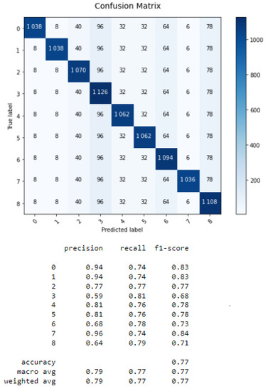
Figure 1.
Confusion matrix of KNN.
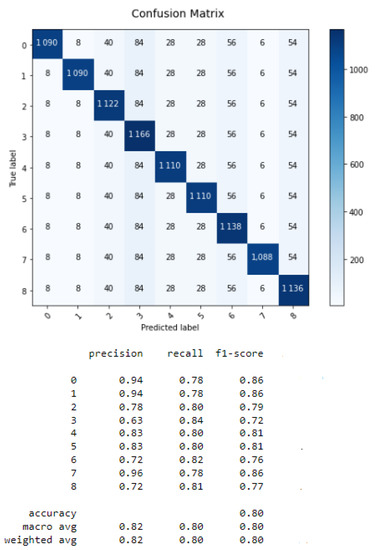
Figure 2.
Confusion matrix of SVM.
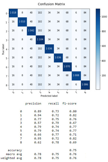
Figure 3.
Confusion matrix of DT.
For the KNN algorithm, the processing time is 0.007 s, and k is equal to 7. This last value is found by calculating the distance between a point and its neighbors, and the number of closer neighbors gives k.
For the SVM algorithm, the processing time is 0.005 s and the parameter C is equal to 1.0. C is chosen via the cross validation of the data.
For the DT algorithm, the processing time is 0.01 s.
Figure 4 depicts the ROC curves for the KNN, SVM, and DT classifiers.
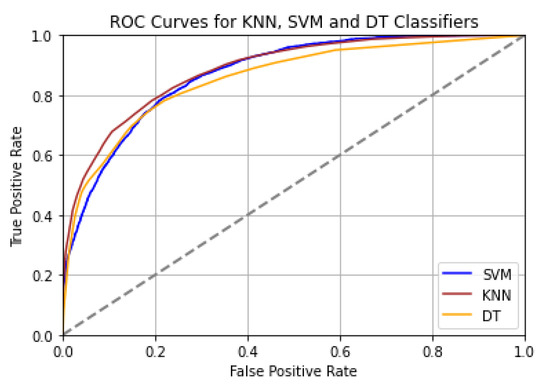
Figure 4.
ROC Curves for KNN, SVM, and DT.
The SVM classifier has the highest AUC-ROC of all the classifiers, as can be seen in Table 1, although 0.87 was not very near 1.

Table 1.
Performance comparison of the models based on AUC-ROC.
Based on Figure 1, Figure 2 and Figure 3, Table 2 presents the error rates of KNN, SVM, DT, and their fusion.
Table 2.
Error rates of the ML classifiers.
As seen from Table 1, the SVM presents the best accuracy and the smallest time processing. However, the use of fused classifiers yields better results than each classifier alone. The best accuracy of 87% is obtained by merging KNN with SVM. The confusion matrix of the fusion of KNN and SVM is given in Figure 5. For the fused classifiers, the time processing is equal to 0.006 s.
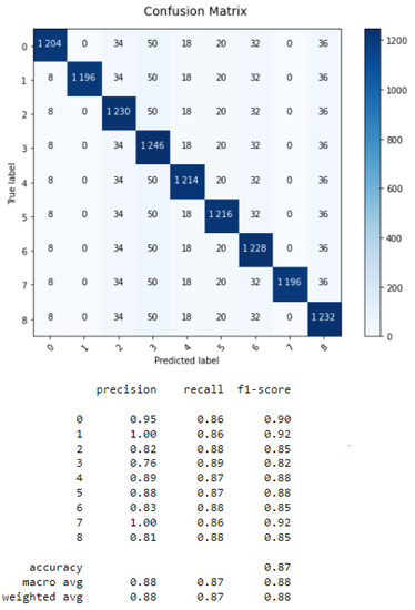
Figure 5.
Confusion matrix of fusing KNN with SVM.
Similarly, for the DL results, the confusion matrices of RNN, CNN, GRU, and LSTM are given by the following figures.
RNN is composed of layers: input with eight neurons, hidden with eight neurons and output layers with two neurons. For RNN, the time processing and the FPS are, respectively, equal to 0.002 s and 25.
CNN is layers of layers namely: a convolutional layer with eight neurons, a maximum pooling layer with four neurons, a flattening layer, a fully connected layer with twelve neurons, and a classification layer with two neurons. For CNN, the time processing and the FPS are, respectively, equal to 0.003 s and 15.
GRU is composed of layers: input with eight neurons, hidden with eight neurons, activation with four neurons, and output layers with two neurons. For GRU, the time processing and the FPS are, respectively, equal to 0.0015 and 30.
For LSTM, the time processing is equal to 0.001.
From Figure 6, Figure 7, Figure 8 and Figure 9, we conclude that the LSTM algorithm provides the best accuracy of 97% with the shortest processing time. The error rates for RNN, CNN, LSTM, and GRU are shown in Table 3.
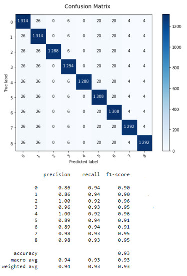
Figure 6.
Confusion matrix of RNN.

Figure 7.
Confusion matrix of CNN.
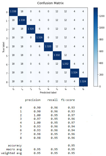
Figure 8.
Confusion matrix of GRU.
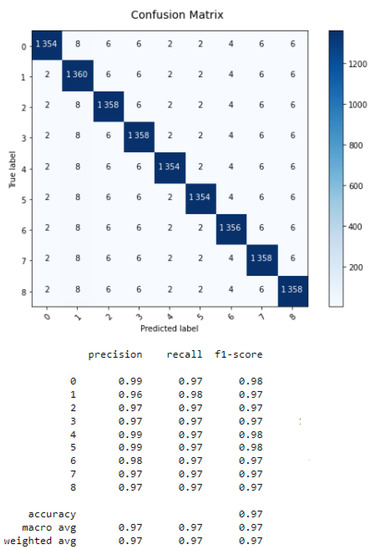
Figure 9.
Confusion matrix of LSTM.
Table 3.
Error rates of DL classifiers.
Figure 10 depicts the ROC curves for CNN, GRU, LSTM, and RNN.
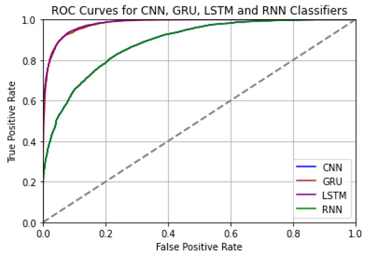
Figure 10.
ROC curves for CNN, GRU, LSTM, and RNN.
The LSTM classifier has the highest AUC-ROC of all the classifiers, as can be seen in Table 4. At 0.99, it is almost equal to 1.
Table 4.
Performance comparison of the models based on AUC-ROC.
To further improve this accuracy, different combinations between the DL classifiers were tested to determine the fusion error rate for each combination; the results are listed in Table 5.
Table 5.
Error rates for fused DL classifiers.
In comparison with Table 2, Table 5 shows that the fusion results based on belief functions are better. For example, the accuracy of with the RNN alone is 93%, whereas that with the combined RNN and GRU is 96%. Similarly, classification with a CNN provides an error rate of 0.1. This rate reduces when the CNN is fused with RNN, GRU, and LSTM.
Based on Table 5, we demonstrate that the accuracy improves by combining LSTM with GRU, reaching 98% with 0.001 s processing time, as shown in its confusion matrix in Figure 11. This result demonstrates the efficiency of the DS theory because it outperformed the other results obtained with each classifier alone (97% obtained from the LSTM classification). In addition, DL provided better accuracy and processing time (98%) than ML (87%). In terms of time and speed, the fusion approach with DL algorithms presents shorter processing time (0.001 s) than with ML (0.006 s). This demonstrates the good performance and power of these algorithms.

Figure 11.
Confusion matrix of fusion LSTM with GRU.
Furthermore, compared with the literature [8,10,14,15,16] where the authors used the same dataset, we can conclude that the obtained accuracy (98%) was improved.
For examples, in [10], the authors studied the same problem based on ML algorithms and using DS theory. The best accuracy was achieved by combining the multilayer perceptron with SVM, but it reached 81%.
In [8], the authors applied four different models, convolutional long short-term memory (Conv-LSTM), CNN-LSTM, traditional LSTM (T-LSTM), and CNN, to classify diabetic patients. These models were applied on the mentioned dataset in two different ways: keeping the training and testing data separate and using five-fold cross validation to evaluate the models. The results showed that each of the four models performed better when the five-fold cross-validation technique was used instead of splitting the dataset for training and testing. The Conv-LSTM model performed better than the other three models in term of accuracy, which achieved 97.26%. For this paper, we note that the uncertainty aspect is not studied.
6. Conclusions
Diabetes is a chronic health problem with severe adverse effects on human life. The challenge of this paper was achieving the early detection of diabetes using classification algorithms. In this framework, two axes are presented. The first one gave a brief description of several ML and DL algorithms, specifying their advantages and disadvantages, principles, and fields of application. This can help the readers to understand better these algorithms that are applied in the field of AI in many sectors. In this case, these classifiers were applied to the problem of diabetes diagnosis in order to determine the best classifiers in terms of accuracy and performance to detect and classify if patients are diabetic or not. Hence, we conducted a comparative study based on the ML classifiers KNN, SVM, and DT and the DL classifiers RNN, CNN, LSTM, and GRU to obtain high-performance precision.
The precision is related to the data used in the learning phase, which always suffers from a level of uncertainty; to overcome the limitation, the second axis used DS theory, which led to fusing the outputs of the ML and DL classifiers in order to improve the quality and reliability of the data and consequently to further improve the obtained accuracy.
The comparative study applied to diabetes tested the ML and DL algorithms with and without considering uncertainty. The results show that the DS theory applied to the combined classifiers yielded better results (98%) compared with the individual classifiers. In addition, the DL algorithms showed better performance compared with the ML algorithms. In the latter, based on some examples, we showed that our results outperformed those obtained in literature.
Thus, we propose using richer databases of attributes. Moreover, applying the attention mechanism to DL algorithms may improve their accuracy.
Author Contributions
Conceptualization, A.E. and M.K.; methodology, O.K.; software, B.K.; validation, H.A., A.A. and M.K.; formal analysis, A.E.; investigation, H.A.; resources, A.A.; data curation, B.K.; writing—original draft preparation, A.E.; writing—review and editing, O.K.; vis-ualization, A.E.; supervision, H.A.; project administration, O.K.; funding acquisition, O.K. All authors have read and agreed to the published version of the manuscript.
Funding
This research has been funded by Scientific Research Deanship at University of Ha’il—Saudi Arabia through project number RG-20 176.
Data Availability Statement
Not applicable.
Conflicts of Interest
The authors declare no conflict of interest.
References
- Ongsulee, P. Artificial Intelligence, Machine Learning and Deep Learning. In Proceedings of the International Conference on ICT and Knowledge Engineering, Bangkok, Thailand, 22–24 November 2017; pp. 22–24. [Google Scholar]
- Frier, B.M. How hypoglycaemia can affect the life of a person with diabetes. Diabetes Metab. Res. Rev. 2008, 24, 87–92. [Google Scholar] [CrossRef] [PubMed]
- Liu, L.; Yager, R.R. Classic Works of the Dempster-Shafer Theory of Belief Functions: An Introduction; Springer: Berlin/Heidelberg, Germany, 2008; pp. 1–34. [Google Scholar]
- Available online: https://fr.statista.com/statistiques/570844/prevalence-du-diabete-dans-lemonde/#statisticContainer (accessed on 22 November 2017).
- Zhou, H.; Myrzashova, R.; Zheng, R. Diabetes prediction model based on an enhanced deep neural network. EURASIP J. Wirel. Commun. Netw. 2020, 2020, 148. [Google Scholar] [CrossRef]
- Ayon, S.I.; Islam, M.M. Diabetes Prediction: A Deep Learning Approach. Int. J. Inf. Eng. Electron. Bus. 2019, 2, 21–27. [Google Scholar]
- Mhaskar, H.; Pereverzyev, S.M. Deep Learning Approach to Diabetic Blood Glucose Prediction. Front. Appl. Math. Stat. 2017, 3, 14. [Google Scholar] [CrossRef]
- Rahman, M.; Islam, D.; Mukti, R.J.; Saha, I. A deep learning approach based on convolutional LSTM for detecting diabetes. Comput. Biol. Chem. 2020, 88, 107329. [Google Scholar] [CrossRef]
- Tymchenko, B.; Marchenko, P.; Spodarets, D. Deep Learning Approach to Diabetic Retinopathy Detection. In Proceedings of the 9th International Conference on Pattern Recognition Applications and Methods—ICPRAM, Valletta, Malta, 22–24 February 2020; pp. 501–509. [Google Scholar]
- Ksantini, M.; Ben Hassena, A.; Delmotte, F. Comparison and fusion of classifiers applied to a medical diagnosis. In Proceedings of the International Multi-Conference on Systems, Signals & Devices, Marrakech, Morocco, 28–31 March 2017; pp. 28–31. [Google Scholar]
- Lichman, M. UCI Machine Learning Repository. 2013. Available online: http://archive.ics.uci.edu/ml (accessed on 17 August 2022).
- Bloch, I. Fusion of Information under Imprecision and Uncertainty, Numerical Methods, and Image Information Fusion. In Multisensor Data Fusion; Springer: Berlin/Heidelberg, Germany, 2002; pp. 267–294. [Google Scholar]
- Ennaceur, A.; Elouedi, Z.; Lefevre, E. Reasoning under uncertainty in the AHP method using the belief function theory. In Proceedings of the 14th International Conference on Information Processing and Management of Uncertainty in Knowledge-Based Systems (IPMU’2012), Catania, Italy, 9–13 July 2012; pp. 373–382. [Google Scholar]
- Srivastava, S.; Sharma, L.; Sharma, V.; Kumar, A.; Darbari, H. Prediction of diabetes using artificial neural network approach. In Engineering Vibration, Communication and Information Processing; Springer: Berlin/Heidelberg, Germany, 2019; pp. 679–687. [Google Scholar]
- Chowdary, P.B.K.; Kumar, R.U. An Effective Approach for Detecting Diabetes using Deep Learning Techniques based on Convolutional LSTM Networks. Int. J. Adv. Comput. Sci. Appl. (IJACSA) 2021, 12. [Google Scholar] [CrossRef]
- Madan, P.; Singh, V.; Chaudhari, V.; Albagory, Y.; Dumka, A.; Singh, R.; Gehlot, A.; Rashid, M.; Alshamrani, S.S.; AlGhamdi, A.S. An Optimization-Based Diabetes Prediction Model Using CNN and Bi-Directional LSTM in Real-Time Environment. Appl. Sci. 2022, 12, 3989. [Google Scholar] [CrossRef]
- Dempster, A.P. Upper and lower probabilities induced by a multivalued mapping. Ann. Math. Stat. 1967, 38, 325–339. [Google Scholar] [CrossRef]
- Shafer, G. A Mathematical Theory of Evidence; Princeton University Press: Princeton, NJ, USA, 1976. [Google Scholar]
- Saravanan, R.; Sujatha, P. A State of Art Techniques on Machine Learning Algorithms: A Perspective of Supervised Learning Approaches in Data Classification. In Proceedings of the International Conference on Intelligent Computing and Control Systems (ICICCS), Madurai, India, 14–15 June 2018. [Google Scholar]
- Osisanwo, F.Y.; Akinsola, J.E.T.; Awodele, O.; Hinmikaiye, J.O.; Olakanmi, O.; Akinjobi, J. Supervised Machine Learning Algorithms: Classification and Comparison. Int. J. Comput. Trends Technol. (IJCTT) 2017, 48, 128–138. [Google Scholar]
- Caruana, R.; Mizil, A.N. An empirical comparison of supervised learning algorithms. In Proceedings of the 23rd International Conference on Machine Learning, Pittsburgh, PA, USA, 25–29 June 2006; pp. 161–168. [Google Scholar]
- Jiao, L.; Pan, Q.; Feng, X.; Yang, F. An evidential k-nearest neighbor classification method with weighted attributes. In Proceedings of the 2013 16th International Conference on Information Fusion (FUSION), Istanbul, Turkey, 9–12 July 2013; pp. 145–150. [Google Scholar]
- Yildiz, T.; Yildirim, S.; Altilar, D.T. Spam Filtering with Parallelized KNN Algorithm; Akademik Bilisim: Istanbul, Turkey, 2008. [Google Scholar]
- Cover, T.M.; Hart, P.E. Nearest Neighbour Pattern Classification. Inst. Electr. Electron. Eng. Trans. Inf. Theory 1967, 13, 21–27. [Google Scholar]
- Fogarty, T.C. First nearest neighbor classification on Frey and Slate’s letter recognition problem. Mach. Learn. 1992, 9, 387–388. [Google Scholar] [CrossRef]
- Shukran, M.A.M.; Khairuddin, M.A.; Maskat, K. Recent trends in data classifications. In Proceedings of the International Conference on Industrial and Intelligent Information, Pune, India, 17–18 November 2012; Volume 31. [Google Scholar]
- Jakkula, V. Tutorial on Support Vector Machine (SVM); Washington State University, School of EECS: Pullman, WA, USA, 2006. [Google Scholar]
- Vapnik, V. The Nature of Statistical Learning Theory; Springer Science & Business Media: Berlin/Heidelberg, Germany, 2013. [Google Scholar]
- Cristianini, N.; Shawe, J. An Introduction to Support Vector Machines and Other Kernel-Based Learning Methods; Cambridge University Press: Oxford, UK, 2000. [Google Scholar]
- Xu, P.; Davoine, F.; Zha, H.; Denœux, T. Evidential calibration of binary SVM classifiers. Int. J. Approx. Reason. 2016, 72, 55–70. [Google Scholar] [CrossRef]
- Bryson, O.; Muata, K. Evaluation of decision trees: A multi-criteria approach. Comput. Oper. Res. 2004, 31, 1933–1945. [Google Scholar] [CrossRef]
- Priyama, A.; Guptaa, R.; Ratheeb, A.; Srivastavab, S. Comparative Analysis of Decision Tree Classification Algorithms. Int. J. Curr. Eng. Technol. 2013, 3, 334–337. [Google Scholar]
- Pouyanfar, S.; Sadiq, S.; Yan, Y.; Tian, H.; Tao, Y.; Reyes, M.P.; Shyu, M.-L.; Chen, S.-C.; Iyengar, S.S. A Survey on Deep Learning. ACM Comput. Surv. 2019, 51, 1–36. [Google Scholar] [CrossRef]
- Shrestha, A.; Mahmood, A. Review of Deep Learning Algorithms and Architectures. IEEE Access 2019, 7, 53040–53065. [Google Scholar] [CrossRef]
- Lauzon, F.Q. An introduction to deep learning. In Proceedings of the International Conference on Information Science, Signal Processing and their Applications (ISSPA), Montreal, QC, Canada, 2–5 September 2012. [Google Scholar]
- Mathew, A.; Amudha, P.; Sivakumari, S. Deep Learning Techniques: An Overview. Adv. Intell. Syst. Comput. 2020, 1141, 599–608. [Google Scholar]
- Dong, S.; Wang, P.; Abbas, K. A survey on deep learning and its applications. Comput. Sci. Rev. 2021, 40, 100379. [Google Scholar] [CrossRef]
- Wu, Q.; Liu, Y.; Li, Q.; Jin, S.; Li, F. The application of deep learning in computer vision. In Proceedings of the 2017 Chinese Automation Congress (CAC), Jinan, China, 20–22 October 2017. [Google Scholar]
- Mouha, R.A. Deep Learning for Robotics. J. Data Anal. Inf. Process. 2021, 9. [Google Scholar] [CrossRef]
- Piccialli, F.; Di Somma, V.; Giampaolo, F.; Cuomo, S.; Fortino, G. A survey on deep learning in medicine: Why, how and when? Inf. Fusion 2020, 66, 111–137. [Google Scholar] [CrossRef]
- Alzubaidi, L.; Zhang, J.; Humaidi, A.J.; Al-Dujaili, A.; Duan, Y.; Al-Shamma, O.; Santamaría, J.; Fadhel, M.A.; Al-Amidie, M.; Farhan, L. Review of deep learning: Concepts, CNN architectures, challenges, applications, future directions. J. Big Data 2021, 8, 1–74. [Google Scholar] [CrossRef] [PubMed]
- Zhang, G. Neural networks for classification: A survey. IEEE Trans. Syst. 2000, 30, 451–462. [Google Scholar] [CrossRef]
- Pietro, R.D.; Hager, G.D. Deep Learning: RNNs and LSTM Handbook of Medical Image Computing and Computer Assisted Intervention; Academic Press: Cambridge, MA, USA, 2020; pp. 503–519. [Google Scholar]
- Kumaraswamy, B. Neural networks for data classification. In Artificial Intelligence in Data Mining; Academic Press: Cambridge, MA, USA, 2021; pp. 109–131. [Google Scholar]
- Li, Y.; Lu, Y. Detection Approach Combining LSTM and Bayes. In Proceedings of the International Conference on Advanced Cloud and Big Data (CBD), Suzhou, China, 21–22 September 2019; pp. 180–185. [Google Scholar]
- Mateus, B.C.; Mendes, M.; Farinha, J.T.; Assis, R.; Cardoso, A.M. Comparing LSTM and GRU Models to Predict the Condition of a Pulp Paper Press. Energies 2021, 14, 6958. [Google Scholar] [CrossRef]
- Chung, J.; Gulcehre, C.; Cho, K.; Bengio, Y. Empirical Evaluation of Gated Recurrent Neural Networks on Sequence Modeling. arXiv 2014, arXiv:1412.3555. [Google Scholar]
- Li, W.; Logenthiran, T.; Woo, W.L. Multi-GRU prediction system for electricity generation’s planning and operation. IET Gener. Transm. Distrib. 2019, 13, 1630–1637. [Google Scholar] [CrossRef]
- Yamak, P.T.; Yujian, L.; Gadosey, P.K. A Comparison between ARIMA, LSTM, and GRU for Time Series Forecasting. In Proceedings of the 2019 2nd International Conference on Algorithms, Computing and Artificial Intelligence, Sanya, China, 20–22 December 2019; pp. 49–55. [Google Scholar]
- Bloch, I. Some aspects of Dempster-Shafer evidence theory for classification of muti-modality medical images taking partial volume effect into account. In Pattern Recognition Letters; Elsevier: Amsterdam, The Netherlands, 1996; pp. 905–919. [Google Scholar]
- Bloch, I. Fusion D’informations en Traitement du Signal et des Images; Hermes Science Publication: Paris, France, 2003. [Google Scholar]
- Dubois, D.; Prade, H. Possibility theory and data fusion in poorly informed environments. Control Eng. Pract. 1994, 2, 811–823. [Google Scholar] [CrossRef]
- Lefevre, E.; Colot, O.; Vannoorenberghe, P. Belief function combination and conflict management. Inf. Fusion 2002, 3, 149–162. [Google Scholar] [CrossRef]


Publisher’s Note: MDPI stays neutral with regard to jurisdictional claims in published maps and institutional affiliations. |
© 2022 by the authors. Licensee MDPI, Basel, Switzerland. This article is an open access article distributed under the terms and conditions of the Creative Commons Attribution (CC BY) license (https://creativecommons.org/licenses/by/4.0/).