

Research on the Optimization of Fresh Agricultural Products Trade Distribution Path Based on Genetic Algorithm

1
School of Management, Dalian Polytechnic University, Dalian 116034, China
2
School of Marxism, Liaoning Normal University, Dalian 116029, China
*
Authors to whom correspondence should be addressed.
Agriculture 2022, 12(10), 1669; https://doi.org/10.3390/agriculture12101669
Submission received: 2 September 2022
/
Revised: 2 October 2022
/
Accepted: 5 October 2022
/
Published: 11 October 2022
(This article belongs to the Special Issue Digital Innovations in Agriculture)
Abstract
:This study, taking the R fresh agricultural products distribution center (R-FAPDC) as an example, constructs a multi-objective optimization model of a logistics distribution path with time window constraints, and uses a genetic algorithm to optimize the optimal trade distribution path of fresh agricultural products. By combining the genetic algorithm with the actual case to explore, this study aims to solve enterprises’ narrow distribution paths and promote the model’s application in similar enterprises with similar characteristics. The results reveal that: (1) The trade distribution path scheme optimized by the genetic algorithm can reduce the distribution cost of distribution centers and improve customer satisfaction. (2) The genetic algorithm can bring economic benefits and reduce transportation losses in trade for trade distribution centers with the same spatial and quality characteristics as R fresh agricultural products distribution centers. According to our study, fresh agricultural products distribution enterprises should emphasize the use of genetic algorithms in planning distribution paths, develop a highly adaptable planning system of trade distribution routes, strengthen organizational and operational management, and establish a standard system for high-quality logistics services to improve distribution efficiency and customer satisfaction.
1. Introduction
With the rapid development of modern society and the economy, people’s living and consumption levels are increasing, and the consumption concept and consumption ideals are also gradually being upgraded. In addition, the demand level for personal dimension is rising. In terms of diet, people pursue a diversity of food choices and high-quality food. Therefore, health food, green food, and other food ration products catering to consumers came into being (as shown in Figure 1 and Figure 2) (Source from “Food consumption trends in leading world markets”. www.statista.com, accessed on 1 October 2022). In reality, consumers’ requirements for fresh produce are gradually changing. The market has shown a trend toward personalized and diversified development. However, fresh agricultural products’ corrosive, regional, and seasonal characteristics have put forward very demanding requirements for logistics and distribution. These characteristics restrict the choice of distribution routes and the transportation time of vehicles. The distribution center is an essential link to modern logistics trade activities. It can improve logistics and distribution efficiency by optimizing logistics and trade distribution paths to reduce logistics and distribution costs. According to incomplete statistics, more than 500 million tons of fresh agricultural products need to be distributed in China, and this value is gradually increasing. As the business scale of various fresh agricultural products logistics and distribution companies continues to expand, consumers’ requirements for logistics service quality are growing higher and higher. At the same time, while emphasizing the freshness and quality of agricultural products, companies require further reduction of logistics and distribution costs, thus improving distribution efficiency. Therefore, studying fresh produce distribution path optimization with a time constraint is conducive to reducing the operation cost of fresh produce distribution companies and improving logistics and distribution efficiency. Moreover, this study has important theoretical significance and application value for logistics and distribution companies for fresh agricultural products.
The planting pattern has recently changed from traditional family-based garden-style vegetable cultivation to large-scale facility farming. The agricultural logistics market is also changing and developing with it. After more than a decade of development, larger wholesale markets for fresh agricultural products have been established. Distribution centers specializing in fresh agricultural products’ processing, storage, and logistics have also been established. According to this survey, most distribution centers for fresh agricultural products have severe problems with unreasonable distribution route design. The distribution routes of each distribution center are often chosen by the distribution drivers themselves under the regulation of the restricted time, and the maximum time limit. This approach lacks proper planning and scientific arrangements. This has led to rising distribution costs, wasted resources, and decreased customer satisfaction.
Therefore, optimizing the logistics distribution route is of great significance to improving the overall efficiency of the distribution of fresh produce distribution centers. A scientific and reasonable distribution route optimization measure can effectively reduce the distribution costs of the distribution center and reasonably arrange the distribution vehicles. Moreover, this measure can also effectively supervise distribution personnel and improve customer service. Therefore, exploring distribution path optimization of fresh agricultural product distribution centers can build a good brand image of fresh agricultural products. Furthermore, while satisfying the local people’s requirements for the safety and freshness of agricultural products, it also promotes the healthy development of fresh agricultural product distribution enterprises.
Based on the research results at the forefront of academia, this paper innovates on two aspects of research content and research objects, respectively, to improve distribution centers’ distribution efficiency and plan scientific distribution paths.
- Regarding the research content, mathematical models have solved previous optimization problems of distribution paths and are rarely linked with the operation of distribution centers. In this paper, we select real-life examples to investigate the problems of distribution paths and construct optimization models of distribution paths. The case study method can combine the genetic algorithm with the actual situation more effectively, thus making up for the disconnect between theory and practice in the previous study.
- Regarding the research object, this paper aims to address the distribution path optimization problem of fresh agricultural product distribution centers. This research will help promote the application of this model in similar fresh agricultural product distribution enterprises with similar characteristics to solve the problem of narrow distribution paths and high distribution costs.
2. Literature Review
In recent years, more and more scholars have focused on researching fresh produce logistics trade distribution and path optimization problems, which are of great significance in terms of the economical use of agricultural trade resources. From the existing literature, the existing studies are mainly distinguished from two aspects: the study of the influence factors of fresh agricultural product distribution and the diversity of research methods used.
The existing literature is mainly focused on fresh agricultural product logistics distribution. The relevant studies mainly focus on three aspects.
The first aspect is the research on the supply chain. Some scholars focus their research perspective on the impact of the supply chain of fresh agricultural products on distribution efficiency. Dabbene’s research group took optimization of the fresh produce supply chain as a starting point. From a supply chain optimization perspective, the team focused on the impact of variable factors such as crop growth maturity, storage temperature, and humidity during transportation on fresh produce logistics and distribution efficiency [1]. Ruhe Xie performed a SWOT analysis on the wholesale market model, agricultural leading enterprise mode, third-party logistics model, E-commerce model, supermarket docking model, and farmer direct sales model. On this basis, the study constructed a system dynamics model of regional circulation of fresh agricultural products to enhance the stability of urban fresh agricultural products supply and improve circulation efficiency [2]. Ying Ji researched the decision optimization problem of cold chain logistics from the perspective of cost-benefit to address the problem of severe loss of fresh agricultural products in circulation and solved it using an analytical model. The study proves that using IoT technology in the logistics practice of fresh agricultural products can strengthen the construction of cold chain logistics and improve logistics efficiency [3].
Another part of the scholars focuses on the design of the supply chain [4]. Akbari Kasgari designed a copper network and backed up suppliers as a resilience strategy. This study proposed models without backup and with backup for multiple objectives and compares them with each other. The result shows that using the backup model can increase supply chain responsiveness and improve the economic and social performance of the supply chain [5]. M. Kaviyani-Charati developed two Bi-Level Stackelberg Models (BLSMs) under non- and agile conditions in the presence of strategic customers. The team considered retailers and manufacturers competing with each other in a sequential game to determine the optimal production and order quantities and prices with and without agile capabilities [6].
The second aspect is the study of the impact of delivery vehicles and delivery time on fresh produce logistics distribution. Some scholars believe that delivery vehicles and delivery time should be considered [7]. Jiang et al. proposed a mixed integer nonlinear programming model (MINLP) to optimize the harvest time and vehicle-to-consumer routes, significantly reducing the time from harvest to distribution of agricultural products [8]. Song et al. examined the selection of logistics models and their impact on fresh produce logistics and distribution. This team confirmed the effectiveness of standard refrigerated vehicle models in fresh produce logistics and distribution [9].
The third aspect is the study of fresh agricultural product logistics and distribution from the perspective of freshness. Banerjee et al. studied the decrease in the freshness of fresh produce in the retail sector with increasing production dates. The scholars studied the inventory model of perishable items from the initial selling price to the future preservation conditions. Based on this, they constructed a daily demand function and distribution model for perishable goods to reduce sales problems [10]. Yan Bo and others construct a dual-channel fresh agricultural product (FAP) supply chain consisting of retailers and suppliers. This study thoroughly considered the impact of freshness level on the freshness of perishable products and constructed a time-varying demand function based on freshness to achieve the optimal pricing strategy and profitability of the supply chain members under dual-channel [11].
Most of the research methods used in the existing literature focus on distribution path optimization models and solution algorithms.
The first aspect is the research on vehicle capacity and time window constraints. The research team of Hop Van Nguyen considered two objectives, delivery lead time and total transportation cost, under the constraints of vehicle capacity and time window. The team proposed an adaptive inertia weighted particle swarm optimization (AIWPSO) algorithm to handle the case of a large number of delivery customers [12]. Bauernhansl et al. studied the vehicle routing problem with constraints such as time windows and vehicle capacity in depth. They designed a vehicle route preference model to suit the needs of each customer service outlet for simultaneous distribution and pick-up. They used distribution models scientifically and rationally. The model minimizes the cost of logistics and distribution operations and enhances customer satisfaction [13].
The second aspect is the study of logistics route optimization calculation. Exact algorithms have a long tradition in distribution route optimization [14]. Archetti et al. use the branch pricing shear approach to perform an integrated service simultaneously, providing multiple logistics points and different logistics products. This approach subdivides the vehicle routing problem into a vehicle routing optimization model with partitioning to demonstrate the model’s effectiveness [15]. Annelieke C. Baller and others used the branch-and-price-and-cut solution method to solve the vehicle routing problem with outsourcing. The method is used to achieve the minimization of fixed, variable, and outsourced costs of the outsourced fleet [16].
At the same time, new models and research methods have been proposed [17,18,19]. Ellabib and other developers have pioneered the idea of parallel data processing and improved the search characteristics of the algorithm in the use of ant colony computing. The computational search performance was also improved using parallel processing concepts for the ACO algorithm [20]. The team also proposes a new method for solving the fully intuitive fuzzy multi-objective fractional transportation problem. The method transforms the problem into a linear problem through some transformations. The linearized model is then reduced to a concise multi-objective transportation problem using the accuracy function of each objective [21]. M.A. Elsisy and others have proposed a new algorithm for generating the Pareto frontier for bi-level multi-objective rough nonlinear programming problems [22]. E.M. et al. systematically investigated the effect of different road selection strategies (including interchange strategies commonly used in practice) on response times and proposed a novel road selection strategy. The model examines not only the transport of cars individually but also the transport transit process between different cars at selected customer locations, known as intermediate transport consolidation. [23].
In conclusion, most scholars’ main research directions are the multi-objective distribution path optimization models with time window constraints and other hybrid algorithms such as modern heuristics. However, due to the unpredictable nature of the actual distribution environment, theoretical models and algorithms are confronted with new requirements during their practical implementation. In contrast, intelligent hybrid algorithms often have to traverse the entire search space, which can very easily lead to combinatorial destruction of the search, making the problem impossible to realize in a polynomial time frame.
Based on this, this paper attempts to use genetic algorithms to solve the problem of fresh agricultural product distribution path optimization. From the literature mentioned above, cutting-edge scholars have researched respectively fresh agricultural product distribution problems and specific algorithms for path optimization. However, little content has been explored for combining genetic algorithms with practical cases. We hope our study will help fill the gap in this area.
3. Theoretical Mechanism
The distribution path generally refers to the distribution path between the logistics distribution center and different distribution locations [24]. The distribution path problem is also known as the vehicle route problem (VRP), which mainly includes distribution centers, customer points, and distribution networks [25]. Distribution path optimization refers to optimizing the route taken by distribution vehicles [26]. The distribution center will face multiple scattered distribution points in performing distribution tasks and choosing several distribution paths. The trade distribution path optimization problem is characterized by complex conditions, time-varying tasks, and non-linearity between variables, which require specific analysis [27]. The distribution path optimization problems are carefully classified according to different classification features, and the various types are shown in Table 1 [28].
There are also many ways to solve the optimization problem of distribution routes in logistics. A classification of the main exact and heuristic algorithms is shown in Figure 3 [29].
The solution of the forbidden search algorithm is very dependent on the initial solution of the model and is not suitable for solving large-scale problems [30,31]. The simulated annealing algorithm has the advantage of short time consumption and eases handling the combined path solution. However, its ability to calculate the optimal solution is poor, and the parameter settings influence its solution results [32]. The optimal path operation of the ant colony algorithm uses a positive and negative mechanism, which is time-consuming. The algorithm is not conducive to the processing and computation of large-scale data and is prone to stagnation while the algorithm is being computed. The accuracy of its solutions depends on operational experience [33]. In this paper, the genetic algorithm was chosen because it better fits the realistic scenario of this paper. However, the genetic algorithm does not quickly obtain a local best path in solving the best vehicle path due to the slow speed of the optimization operation process.
Nevertheless, the overall best result is better obtained using the genetic algorithm. Due to the slow speed of the optimization operation process, the genetic algorithm is more difficult to obtain the local best path in solving the best path. However, it is easy to arrive at the overall best result. From a holistic perspective, the genetic algorithm has the highest correctness. Combined with the specific situation of this paper’s research, this paper uses genetic algorithms in heuristic algorithms as the research method.
4. Analysis of the Current Situation
4.1. Basic Situation
Jinpu New District of Dalian City has unique geographical advantages. Located in the geographical center of Northeast Asia, the district has traded with more than 300 ports in more than 160 countries and regions, with a total area of 2299 square kilometers and a population of 1.61 million. Dalian Jinpu New Area Fresh Agricultural Product Distribution Center (DJ-FAPDC) is located in the Dalian Jinfadi Comprehensive Wholesale Market (Due to the space limitation, the Dalian Jinpu New Area fresh agricultural product distribution center will be named “DJ-FAPDC” in the following contents of this article for the convenience of reading and explanation. This is to clarify.). Dalian Jinfadi Comprehensive Wholesale Market is the largest comprehensive wholesale market in Dalian. It is located at the intersection of Huaihe West Road and Wutun Airport in Jinzhou District, Dalian, covering an area of more than 400,000 square meters. The wholesale market is developed in two phases, and the agricultural and sideline products trading market is the first phase of construction. It covers an area of 180,000 square meters, with a construction area of 60,000 square meters and 120,000 square meters of roads, parking, and ground hardening. Among them are ten trading halls with an area of 35,520 square meters and six buildings with warehouse gatehouses of 9000 square meters. Other than this, there are four comprehensive supporting buildings for refrigeration and quick freezing, with an area of 14,600 square meters.
In the wholesale market, dozens of small agricultural and sideline products companies and five large fresh agricultural products distribution companies. Among them, R Fresh Product Distribution Center (R-FAPDC), as one of DJ-FAPDC, is the earliest, largest, and most representative distribution center that was established.
4.2. Current Situation and Problems
Through an extensive survey, it was learned that DJ-FAPDC lacks a modern intelligent distribution route planning system. The trade distribution path selection of DJ-FAPDC has the characteristics of randomness and subjectivity, mainly relying on the empirical selection of distribution personnel. This leads to the following problems in the distribution of DJ-FAPDC.
4.2.1. Lack of Standardization in Trade Distribution Route Planning Leads to Higher Distribution Costs
Random logistics and distribution route planning can significantly increase the distribution costs of logistics and distribution centers. A large number of distribution points in each logistics and distribution center results in an excessive number of logistics and distribution routes being chosen. When selecting routes manually will inevitably lead to uncertainty in vehicle mileage and higher distribution costs for logistics and distribution centers.
4.2.2. Lack of Regulation in Distribution Route Planning Leads to Lower Customer Satisfaction
DJ-FAPDC’s customer demands are increasingly characterized by multiple batches, small lots, and urgency. Irrational trade distribution route planning can lead to difficulty handling emergencies and heavy load on distribution vehicles during the distribution process. At the same time, the problem of poor customer service is increasingly exposed, leading to lower customer satisfaction.
4.2.3. Lack of Standardization in Distribution Route Planning Makes it Difficult to Guarantee the Distribution Time
DJ-FAPDC has not planned and designed the distribution routes of distribution vehicles. Therefore, strict time limits cannot be imposed on the distribution time of vehicles. This has led to difficulties for DJ-FAPDC to meet the requirements of vehicle recycling. The difficulty of its management is increased. No vehicle may be available for dispatch when there is a temporary urgent delivery task. In addition, it is also difficult to improve customer satisfaction in such situations.
This shows that DJ-FAPDC pays insufficient attention to distribution route planning and lacks a comprehensive logistics distribution and distribution route planning system. The logistics and distribution center was unable to monitor the status of the implementation of the distribution plan, nor was it able to effectively control the distribution vehicles and staff. DJ-FAPDC’s logistics concept is backward. The specific performance includes the following three aspects. (1) The distribution center did not invest enough in logistics activities, focusing only on producing and selling fresh agricultural products. (2) The distribution center lacks good logistics and trade distribution planning. The distribution companies did not adopt a modern logistics management system. (3) The logistics and distribution department staff lacked knowledge in the logistics field. In their daily work, they can only rely on their work to accumulate experience, which makes them lack scientific theoretical support and unable to make scientific management decisions.
5. Construction of Distribution Path Optimization Model
This paper will start from the perspective of trade distribution path optimization of fresh agricultural products distribution enterprises, taking R-FAPDC as an example. After considering the timeliness of fresh agricultural products, a distribution path optimization model with time window constraints is constructed and solved in this study. The ultimate objective of this study is to help the fresh produce distribution enterprises in the Jinpu New Area of Dalian find the optimal distribution route with the lowest cost, highest efficiency, and excellent customer satisfaction. At the same time, this paper reduces human decision-making errors by employing scientific planning of distribution routes, realizing real-time control of personnel and vehicle dynamics by enterprises, and closing the loopholes of in-transit supervision.
The elements of the simulation scenario in this paper are: to complete the sorting, loading, and unloading of goods at distribution points within the distribution center, plan good routes for distribution personnel, and complete home delivery services. Among them are known: the distribution network, including the geographic location of each customer node and the distance of each section of the route; cargo information, including attributes such as cargo specifications and weight, as well as the delivery time requested by the customer and the acceptable time window; and dispatch information, including the number of vehicles and the maximum load capacity.
5.1. Model Assumptions
In this paper, the model is constructed based on the research of cutting-edge scholars. The goal is to achieve a high degree of integration between genetic algorithms and actual cases, thus improving the model’s practical utility. Reasonable assumptions can simplify the model construction process, reduce the consideration of secondary factors, and reduce the difficulty of model construction. Therefore, to control some unexplained variables and directly reflect the fundamental problems of the model, this study simplifies the actual situation. This paper proposes setting conditions for the appropriate environment required for model construction.
- Distribution point: each distribution point demand is satisfied, and only one distribution transport vehicle is allowed to serve it and be visited only once.
- Distribution vehicles: The distribution vehicles are of uniform type and have the same load and speed.
- Distribution routes: The distribution center has sufficient vehicles to serve each route in time, according to the demand.
- Distribution center: The distribution center is unique and is the starting, and final destination of each distribution vehicle, and no more midway assignments are made.
- Load limit: The total amount of all customer demands on the same path shall not exceed the vehicle’s rated load.
- Time window constraint: The arrival time of delivery vehicles and loading operation shall be satisfied within the acceptable time window of the delivery point. Otherwise, it is invalid.
- Distribution process without consideration of road congestion, bad weather conditions, or vehicle breakdown.
5.2. Symbol Description
The symbols appearing in this paper and their practical meanings are shown in Table 2.
5.3. Distribution Cost Analysis
The distribution cost of the distribution center includes several aspects: transportation, sorting, assembly, and distribution processing. Based on the actual situation of fresh produce distribution in this paper, the sorting, assembly, and distribution processing costs are not the main costs in this paper.
Therefore, they can be disregarded. This paper will consider distribution costs from the following three aspects [34,35].
5.3.1. Fixed Costs
Numbered lists can be added as follows: It refers to costs unrelated to the distance traveled by the vehicle and the number of goods transported within the distribution chain but will undoubtedly be incurred. It includes management costs, repair and maintenance costs, road maintenance fees, bridge fees, and other miscellaneous costs. This part of the cost is only related to the number of vehicles. Thus, the calculation formula is shown below.
where e n denotes the number of vehicles invested in the distribution segment; f1 denotes the fixed cost incurred by each vehicle in the distribution segment.
5.3.2. Transportation Costs
It refers to the part of the cost that increases or decreases with the mileage and vehicle load in the distribution process. It is also known as a vehicle-kilometer variable cost, including fuel consumption and depreciation costs. This cost can be obtained by multiplying the mileage of the distribution vehicle and the transportation cost per unit distance. The calculation formula is shown below.
where Dij denotes the mileage traveled between customer i, j; f2 denotes the transportation cost per unit distance; Xijk is a 0,1 variable, indicating that the kth vehicle completes the delivery operation of customer i, j.
5.3.3. Penalty Costs
Customers often have personalized requirements for delivery time and want to complete the delivery within the specified time window. However, in the actual delivery operation, the delivery operation cannot be completed within the specified time due to objective reasons such as bad weather, traffic jams, or subjective factors such as mistakes in route selection by delivery personnel. Early or late delivery can affect customer satisfaction and bring penalty costs to the delivery company. In this paper, penalty cost is defined as any additional cost to delivery companies due to the impact of delivery time [36]. According to the times, delivery vehicles arrive at customer locations. This paper will analyze penalty costs in three cases: early arrival, on-time arrival, and delayed arrival.
- Early arrival.
Usually, the customer specifies the delivery time, which means that the delivery can only be signed for within a specific period. Therefore, when the vehicle arrives at the customer’s location in advance, it needs to wait until the set time for door-to-door delivery service. In the waiting process, vehicles and human resources will be wasted, equivalent to delivery companies paying extra waiting costs.
- 2.
- On-time arrival.
The door-to-door delivery service can be carried out on time when the vehicle arrives at the customer’s location according to the agreed time. After the customer signs for the delivery, the distribution staff will go to the next destination. There will be no additional cost to the delivery company in this ideal situation.
- 3.
- Delayed arrival.
Due to traffic congestion and human error, the delivery company must pay additional vehicle in-transit costs when the vehicle arrives later than the specified delivery time. Furthermore, the company also needs to bear the cost of possible secondary delivery.
Suppose the time for the kth vehicle to arrive at customer i’s location is [Eik, Lik]. The deliverable time specified by customer i is [ei, li] and is a subset of [Eik, Lik]. The actual vehicle arrival time Aik ∈ [Eik, Lik]. Based on the above three cases for penalty cost generation analysis, a line graph of penalty cost with distribution time is derived, as shown in Figure 6.
In summary, the expression for calculating the penalty cost of the distribution chain is:
- f3 indicates the waiting cost incurred per unit of time in case of early arrival.
- f4 denotes the delayed cost incurred per unit time when arriving late.
- Xik is a 0, 1 variable indicating that the kth vehicle performs the delivery operation for customer i.
5.4. Analysis of Customer Satisfaction
This paper’s distribution path optimization model is a multi-objective function model to achieve the minimum distribution cost and the highest customer satisfaction simultaneously. Therefore, this paper needs to analyze customer satisfaction briefly.
Customer satisfaction refers to the subjective feelings of customers about the products or services they receive. When portraying satisfaction, it is generally the ratio between the expected value and the final achieved value, which is between [0,1]. In the case of delivery services, satisfaction is mainly influenced by whether the delivery company can meet the customer’s requirements for delivery time [37].
5.4.1. Fuzzy Appointment Time
The concept of fuzzy appointment time has emerged in academia because of the uncertainty in real life regarding the setting of delivery time windows by customers. Fuzzy appointment time is the concept of time interval, which contains the customer’s desired service point or time and the range of service time that the customer can tolerate to overrun or delay [38].
When the adequate service time of customer i is a specific time point Ti, the linear image representation of customer satisfaction is shown in Figure 7.
The linear image of customer satisfaction when the satisfied service time of customer i is a specific time [ei, li] is shown in Figure 8.
Customer satisfaction at different time points or periods is shown as follows.
- When the delivery service occurs at the reservation time point Ti or within the time [ei, li], the customer expectation is met, and the satisfaction level reaches the highest.
- When the delivery service does not occur at the reservation time point Ti or within the time [ei, li] but is within the tolerable delivery time window [Ei, Li], the customer’s expectations are not achieved. However, the customer still chooses to accept the service. At this time, customer satisfaction is average.
- When the delivery service occurs outside the tolerable delivery window [Ei, Li], it is far from meeting the customer’s expectations, and customer satisfaction is the lowest.
5.4.2. Time Window-Based Customer Satisfaction Measurement
In the actual delivery process, in most cases, customers will pre-set the delivery time window instead of the scheduled time point. Therefore, this paper’s time window is fuzzy reservation time processing. Concurrently, this paper uses the fuzzy post-affiliation function shown in the following equation to represent customer satisfaction [39,40,41].
The expression for the average customer satisfaction is:
5.5. Model Building
5.5.1. Objective Function
- Treatment of multi-objective function
This paper studies how to achieve the optimal balance between the two objectives of minimizing distribution cost and maximizing customer satisfaction based on satisfying distribution timeliness. This problem belongs to the multi-objective function optimization problem [42]. In order to make the solution more convenient, this study converts the two objective function optimization problems into achieving a single objective function optimization problem. The special treatment is shown below.
In the following, to be consistent with solving the distribution cost minimization objective, this paper converts achieving the maximum average customer satisfaction into solving the minimum average customer dissatisfaction.
- 2.
- Final objective function
5.5.2. Constraints
All models have corresponding conditions of applicability. In order to constrain the generation of its wide range of results and facilitate analytical processing, this study constructs the following constraints for the above models.
- 0-1 variables
- 2.
- The actual weight of the vehicle shall not exceed the maximum weight of the vehicle.
- 3.
- Each customer has only one vehicle to deliver for him/her.
- 4.
- After a delivery task is completed, the delivery vehicle must go to the next delivery point.
- 5.
- The vehicle returns to the distribution center after completing all tasks.
- 6.
- The vehicle capacity fulfills the distribution needs of all customers.
- 7.
- The number of vehicles involved in distribution does not exceed the number of all distribution vehicles.
- 8.
- Meeting the time window constraints of all customers.
6. Case Study of Fresh Produce Distribution Center
6.1. Background Introduction
R-FAPDC is one of the earliest fresh produce distribution enterprises established in the Jinpu New Area. Furthermore, it is also one of the critical leading companies of agricultural industrialization in the Dalian Jinpu New Area. The distribution center was built in 2005. It has a freezing processing warehouse of 1000 m2, a distribution center of 2000 m2, a vegetable planting base of 333,335 m2, and 86 employees. In addition, the distribution center has 13 vehicles in charge of distribution, and the vehicle types are all light vans. Among them, the total vehicle mass is 4500 kg, and the load capacity is 1500 kg.
6.2. Data Collection and Processing
6.2.1. Constraints
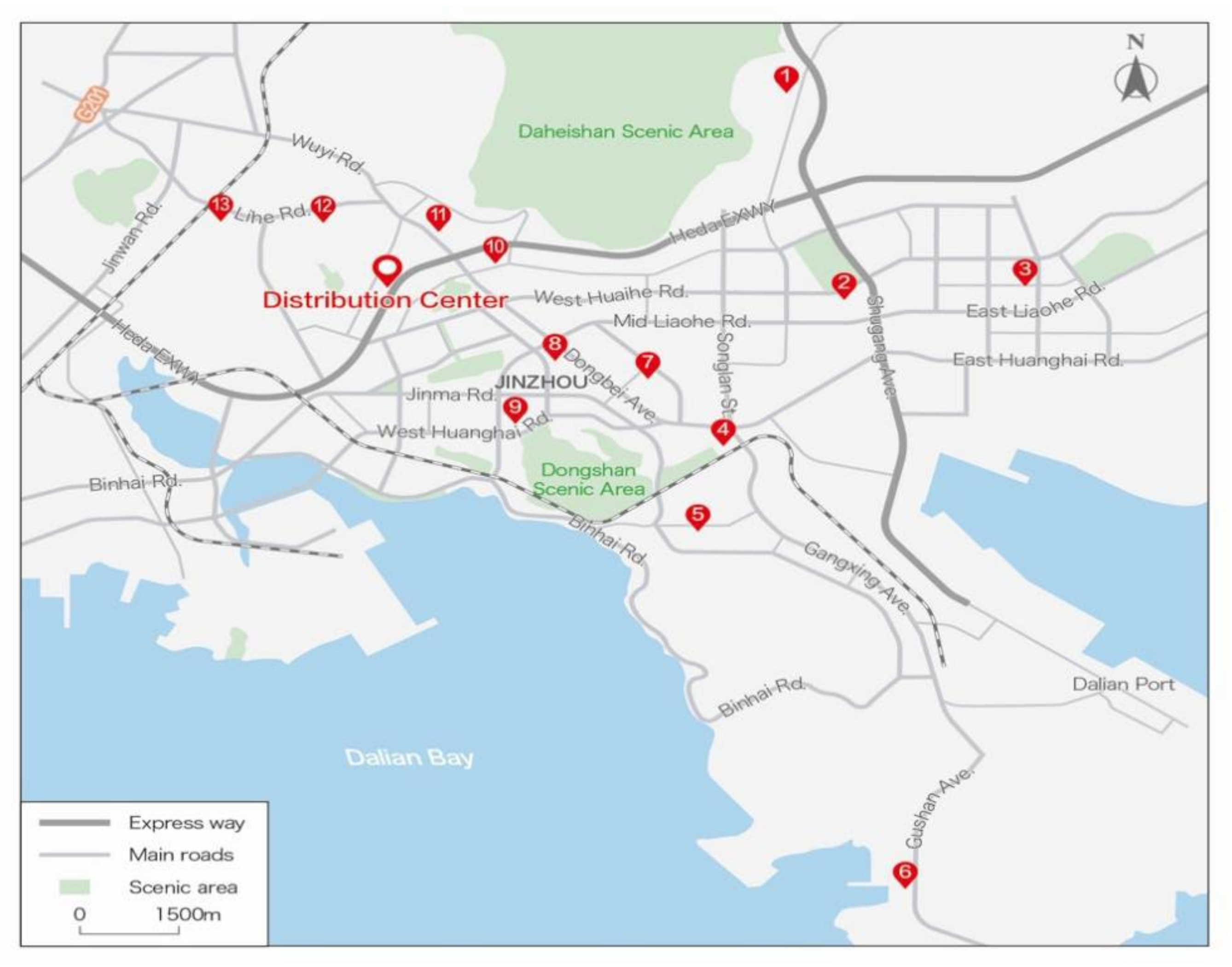
The main distribution area of R-FAPDC is 13 distribution areas in Jinpu New District. The locations of distribution points are shown in Figure 9.
6.2.2. Addresses and Codes of Distribution Points
The addresses and codes of R-FAPDC and 13 distribution points are shown in Table 3.
6.2.3. Distribution Point Data Information
This paper retrieved relevant information through the distribution center sales system during the research period. This paper can obtain the distance and demand information of 13 distribution outlets in R-FAPDC. The summary is shown in Table 4.
The distance information between distribution outlets is shown in Table 5.
6.2.4. Demand Time Window
It refers to the best service time acceptable to the customer and the tolerable delivery time. This method requires converting the time format of the time window to a decimal format that is convenient for algorithmic operations. Example: “06:00” is converted to “06.00”. The results of the conversion are shown in Table 6.
6.2.5. Other Parameters
To simplify the operation, this study takes the median value of each parameter interval to fix the parameters, as shown in Table 7.
6.3. Algorithm Parameter Setting
According to the actual situation of the calculation case, in this paper, if we want to simplify the operation based on the validity of the solution results, we need to set the algorithm parameters. The specific parameter settings are shown in Table 8.
6.4. Model Solving
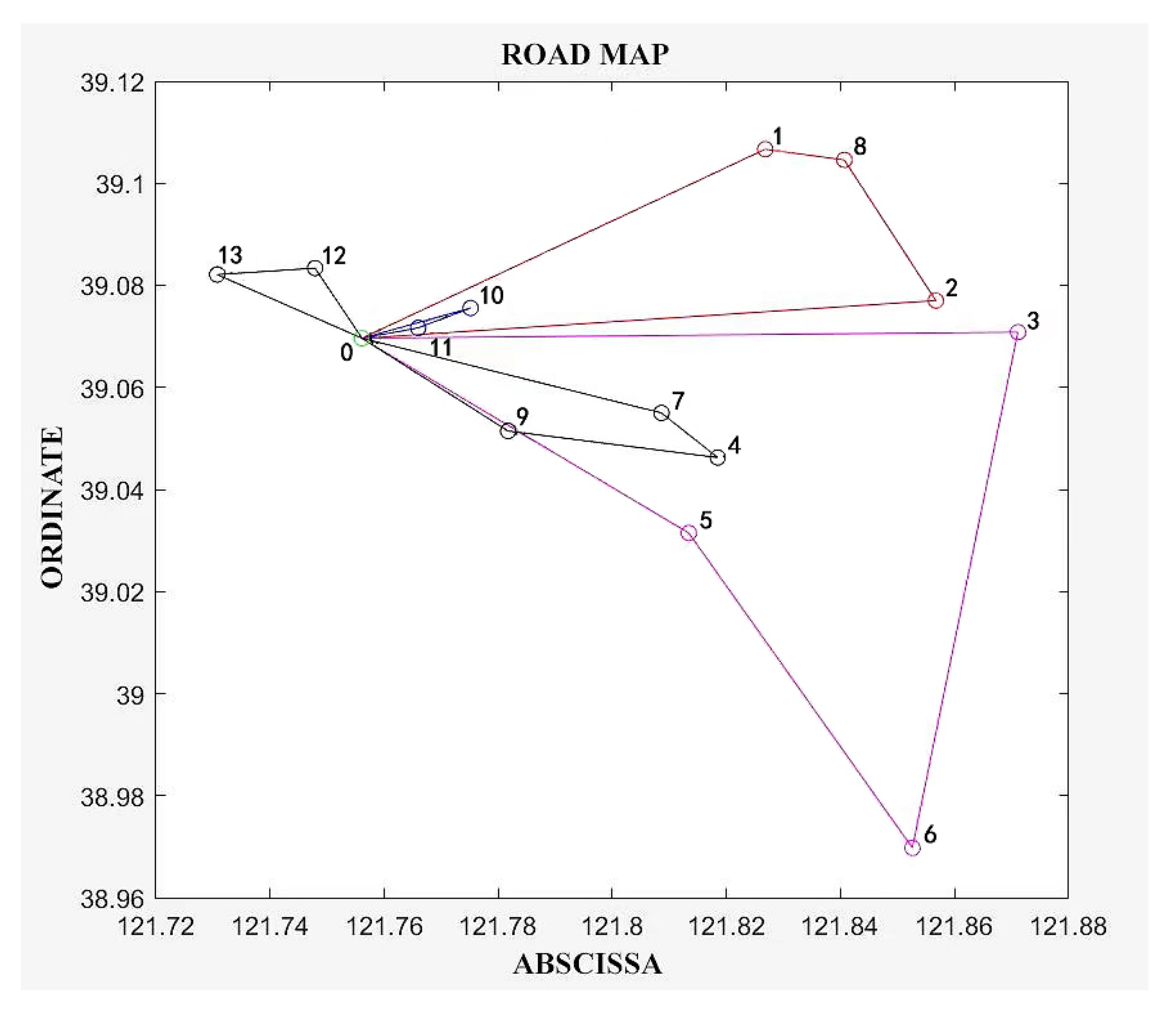
We substitute the collated data and the set parameters into the model constructed in the previous chapter and use MATLAB computer software to program the solution. Through simulation experiments on the distribution path of R-FAPDC, the final cost iteration diagram and path diagram after path optimization are derived, as shown in Figure 10 and Figure 11.
The specific route selection after optimization is shown in Table 9.
6.5. Comparative Analysis before and after Optimization
The initial distribution routes before optimization are shown in Table 10.
Before optimization, the distribution vehicle dispatching details are shown in Table 11, Table 12 and Table 13.
The optimized path diagram clearly shows that the distribution center needs 5 vehicles to complete the distribution tasks in the distribution chain. The scheduling and usage details of the corresponding distribution vehicles are shown in Table 14, Table 15 and Table 16.
The detailed comparison results before and after distribution path optimization are shown in Table 17.
After various cost calculations, the results show that the distribution center must dispatch five transport vehicles in the distribution chain. The total cost of distribution at this stage is 1074.4 RMB, compared with the total cost corresponding to the distribution path before optimization, which is 1294.4 RMB, a reduction of 220 RMB. Among them, the fixed cost savings accounted for 68% of the total cost savings; the transportation cost savings accounted for 14% of the total cost savings; the penalty cost savings accounted for 18% of the total cost savings. The improved delivery path can save 33 min compared to the pre-improved delivery path. The average loading rate of the six transport vehicles before optimization was 68%, and the average loading rate of the five transport vehicles after optimization was 82%. The vacancy rate of distribution vehicles is low.
The comparison results show that the model constructed in this paper is reasonable and practical. Optimized trade distribution routes can help distribution companies reduce costs, including transportation costs and penalty costs. Concurrently, customer satisfaction can be improved.
7. Conclusions and Prospects
7.1. Conclusions
With the growing demand for fresh agricultural products trade, the research about fresh agricultural products distribution and the business of fresh agricultural products logistics distribution has been developing rapidly. What cannot be ignored is that trade distribution has gradually shifted from a single route to an interactive network. This has also led the fresh produce distribution centers to enter a critical period of rapid development in multiple ways. They have more paths and ways of choice possibility. Through the case analysis and comparison results derived from the above model, this study draws the main conclusions based on the theory related to distribution path optimization. The results of the study include that:
- Due to the expansion of the distribution network of distribution centers, the previous method of judging distribution paths based on manual experience can no longer adapt to the growing fresh agricultural product distribution centers.
- R-FAPDC has its value. It has the typical characteristics of fresh trade distribution in coastal areas. Suppose the distribution problem research of such object considers the particular timeliness of fresh agricultural products distribution, constructs a multi-objective distribution path optimization model with time window constraints, and uses the genetic algorithm to derive a reasonable distribution route that meets the independent characteristics. In that case, it will be of great significance to improve the efficiency of trade distribution.
The results of this paper reveal that:
- The trade distribution path scheme optimized by the genetic algorithm can reduce the distribution cost of fresh agricultural products distribution centers and improve customer satisfaction.
- The genetic algorithm can bring economic benefits and reduce transportation losses in trade for the trade distribution centers with the same spatial characteristics and quality characteristics as R-FAPDC.
Therefore, the above conclusion shows that the genetic algorithm is effective for the optimization scheme of trade distribution path for fresh agricultural products distribution centers and has reference significance for other similar problems.
7.2. Data Collection and Processing
7.2.1. Emphasis on the Use of Genetic Algorithms in Planning Trade Distribution Path
The genetic algorithm has excellent advantages. We have analyzed land transportation traffic in a vital development zone in the Northeast Asia International Shipping Center compared with other studies, considering various complex possibilities. Moreover, in this study, the genetic algorithm ensures the diversity of the distribution path population and the overall population quality and suppresses the algorithm’s premature search. The use of this algorithm is more conducive to obtaining the optimal global solution and optimal distribution paths. The comparison with the original internal data of the company confirms the idea of “effectiveness.” Therefore, we suggest paying attention to the use of genetic algorithms in planning trade distribution paths and applying them to a broader range of problems. This is a trend to be considered.
7.2.2. Development of a Planning System of Trade Distribution Routes with High Adaptability
The distribution route planning system is crucial for a fresh produce distribution company. At a time when the modern trade process cycle is growing shorter and shorter, each trade link’s efficiency is becoming more and more demanding. Companies largely ignore distribution problems, and their random and unexpected nature makes it even less easy to control costs. Therefore, a stable planning system of trade distribution route is related to the cost saving and profit growth or even the quality of the whole trade link completion. The function of the distribution route planning system is not only route planning but also covers all the links in the trade distribution supply chain. Distribution route planning is only one of the functions, but it is also essential. When used well by enterprises, it can significantly improve fresh food companies’ delivery speed and efficiency [43]. Compared to manual experience, scientific system planning is more reasonable. This paper provides a model framework and demonstrates its initial effectiveness in improving trade distribution efficiency and reducing distribution costs. It also provides a reference for developing respective planning systems of trade distribution routes.
7.2.3. Strengthening the Rational Setting of Worker Performance in the Management of Organizational Operations
People are the root of all productive forces. This means that people can determine productivity and production relations. That is not to mention the power of a single worker in handling the resources of the company to which he belongs without constraints [44]. If workers are motivated through a performance setting, it will surely increase resource-saving efficiency. Therefore, fresh produce distribution centers should form a reasonable organizational structure. Based on an effective organizational structure, the distribution company should use a performance management model throughout each link, from production to sales. For example, distribution centers ought to implement operational handling performance management in the sorting segment, performance management of trade distribution efficiency in the distribution segment, and sales performance management in the sales segment [45]. In this way, it helps the staff be willing to work and think about company profitability and saving. In addition, the distribution center should regularly train the staff with professional knowledge and skills to help them combine their professional knowledge and work experience effectively and thus improve their distribution efficiency.
7.2.4. Establishing a High-Quality Logistics Service Standard System to Realize the Benign Development of Enterprise Distribution Work in the Process of Winning Customers
A high-quality logistics trade service standard system can not only improve the service level of distribution centers and optimize the business process of the distribution system but also significantly improve the efficiency of logistics and distribution to promote the smooth and sound development of fresh agricultural products distribution centers. It is the next development trend in logistics and distribution of distribution centers. Through standardized means, enterprises standardize service concepts, integrate service functions, and promote service equipment, to finally realize the standardized management of fresh agricultural products distribution centers.
8. Deficiencies and Prospects
8.1. Deficiencies
In this paper, a representative R-FAPDC in Jinpu New District, Dalian, is selected as an arithmetic example, and its distribution path is optimized using a genetic algorithm. Satisfactory results are finally obtained. However, this is an experimental result obtained by simulation under certain assumptions and constraints. Furthermore, the experiment eventually has to return to reality. In real life, it is often disturbed by many external factors. The subsequent research needs to consider various external influences more comprehensively.
- Some specific conditional restrictions are proposed in the model assumptions section. For example, all delivery vehicles are the same model, and the customer demand at the delivery point is always the same.
- In the data collection part, the customer demand information is mainly derived from the system records of R-FAPDC. This is a real-time data record. The distribution of data information may change at any time, which in turn affects the optimization effect. In this paper, the supply information of distribution nodes is known in advance. However, in reality, the supply quantities of distribution points are uncertain. This may lead to unforeseen new problems when implementing specific solutions.
- The optimized distribution path scheme is not implemented in practice in this paper due to the time constraints of the study and personal and professional levels. Therefore, the specific implementation effects in the distribution environment have not been studied in depth.
8.2. Prospects
This paper constructs a multi-objective distribution path optimization model with time windows based on the research of frontier scholars. Preliminary research results have been achieved using a genetic algorithm optimization solution. However, with the continuous development of society, it is necessary to continuously enrich, improve, and develop the theory to carry out subsequent research work.
- Subsequent research should continuously optimize the algorithm. This paper only uses the genetic algorithm for path optimization solutions. There are many path optimization algorithms. Each algorithm has its advantages and disadvantages. Solving such problems with a single algorithm will inevitably have drawbacks and defects. The next step can be to improve the genetic algorithm or combine the genetic algorithm with other heuristic algorithms.
- The distribution center should use modern intelligent technology to monitor the distribution process. In the future implementation of the distribution plan, consider in-depth research in supervising the distribution process and grasping the optimization effect. In particular, with the wide application of IoT (“Internet of Things”) technology, fresh agricultural product distribution centers should use modern intelligent methods to monitor the distribution process effectively.
- Researchers should consider the freshness of agricultural products in the optimization model constraints. The confirmation and measurement of the freshness of the agricultural products are not considered in the distribution process, and no detailed constraints are established. In the following research, it is necessary to further quantify and reflect the freshness of fresh agricultural products in the model to improve the optimization effect comprehensively.
- Researchers should continue to study the main reasons affecting the distribution efficiency in the distribution process, such as congestion or the distribution efficiency affected by the receiving and inspection link. If the delivery time is delayed by the receiving and inspection process, blind matching can be considered. Compare the cost of blind distribution with the previous distribution cost to choose a more reasonable distribution method.
Author Contributions
Writing—original draft preparation, J.S.; writing—review and editing, T.J., Y.S., H.G. and Y.Z. All authors have read and agreed to the published version of the manuscript.
Funding
This research received no external funding.
Institutional Review Board Statement
Not applicable.
Informed Consent Statement
Not applicable.
Data Availability Statement
Due to the confidentiality agreement requirements for the information sources used in this study, only the results are published, and the data sources for comparison are not explained at this time.
Conflicts of Interest
The authors declare no conflict of interest.
References
- Dabbene, F.; Gay, P.; Sacco, N. Optimisation of fresh-food supply chains in uncertain environments, Part I: Background and methodology. Biosyst. Eng. 2008, 99, 348–359. [Google Scholar] [CrossRef]
- Xie, R.; Han, S.; Jiang, Y.; Peng, Z. Comparison and Optimization of Circulation Modes of Fresh Agricultural Products Based on System Dynamics—The Case of China. J. Serv. Sci. Manag. 2018, 11, 297–322. [Google Scholar] [CrossRef] [Green Version]
- Ying, J. Decision Optimization for Cold Chain Logistics of Fresh Agricultural Products under the Perspective of Cost-Benefit. Libr. J. 2019, 6, 1–17. [Google Scholar]
- Taghipour, A.; Khazaei, M.; Azar, A.; Ghatari, A.R.; Hajiaghaei-Keshteli, M.; Ramezani, M. Creating Shared Value and Strategic Corporate Social Responsibility through Outsourcing within Supply Chain Management. Sustainability 2022, 14, 1940. [Google Scholar] [CrossRef]
- Akbari-Kasgari, M.; Khademi-Zare, H.; Fakhrzad, M.B.; Hajiaghaei-Keshteli, M.; Honarvar, M. De-signing a resilient and sustainable closed-loop supply chain network in copper industry. Clean Technol. Environ. Policy 2022, 24, 1553–1580. [Google Scholar] [CrossRef]
- Kaviyani, C.M.; Ghodsypour, S.H.; Hajiaghaei, K.M. Impact of adopting quick response and agility on supply chain compe-tition with strategic customer behavior. Sci. Iran. 2022, 29, 387–411. [Google Scholar]
- Li, M.; He, L.; Yang, G.; Lian, Z. Profit-Sharing Contracts for Fresh Agricultural Products Supply Chain Considering Spatio-Temporal Costs. Sustainability 2022, 14, 2315. [Google Scholar] [CrossRef]
- Jiang, Y.; Chen, L.; Fang, Y. Integrated Harvest and Distribution Scheduling with Time Windows of Perishable Agri-Products in One-Belt and One-Road Context. Sustainability 2018, 10, 1570. [Google Scholar] [CrossRef] [Green Version]
- Song, B.D.; Ko, Y.D. A vehicle routing problem of both refrigerated- and general-type vehicles for perishable food products delivery. J. Food Eng. 2016, 169, 61–71. [Google Scholar] [CrossRef]
- Banerjee, S.; Agrawal, S. Inventory model for deteriorating items with freshness and price dependent demand: Optimal discounting and ordering policies. Appl. Math. Model. 2017, 52, 53–64. [Google Scholar] [CrossRef]
- Yan, B.; Fan, J.; Wu, J.-W. Channel choice and coordination of fresh agricultural product supply chain. RAIRO—Oper. Res. 2021, 55, 679–699. [Google Scholar] [CrossRef]
- Hop, V.N.; Phan, P.P. Adaptive inertia weight particle swarm optimisation for a multi-objective capacitated vehicle routing problem with time window in air freight forwarding. Int. J. Syst. Manag. 2021, 40, 423–442. [Google Scholar]
- Oesterle, J.; Bauernhansl, T. Exact Method for the Vehicle Routing Problem with Mixed Linehaul and Backhaul Customers, Heterogeneous Fleet, time Window and Manufacturing Capacity. Procedia CIRP 2016, 41, 573–578. [Google Scholar] [CrossRef]
- Archetti, C.; Bianchessi, N.; Grazia, S.M. A branch-price-and-cut algorithm for the commodity constrained split delivery ve-hicle routing problem. Comput. Oper. Res. 2015, 64, 1–10. [Google Scholar] [CrossRef] [Green Version]
- Dimitrakos, T.; Kyriakidis, E. A single vehicle routing problem with pickups and deliveries, continuous random demands and predefined customer order. Eur. J. Oper. Res. 2015, 244, 990–993. [Google Scholar] [CrossRef]
- Annelieke, C.B.; Said, D.B.; Wout, E.H.; Dullaert, D.V. The Vehicle Routing Problem with Partial Outsourcing. Transport. Sci. 2020, 54, 855–1152. [Google Scholar]
- El Sayed, M.; Farahat, F.; Elsisy, M. A novel interactive approach for solving uncertain bi-level multi-objective supply chain model. Comput. Ind. Eng. 2022, 169, 108225. [Google Scholar] [CrossRef]
- Elsisy, M.A.; Elsaadany, A.S.; El Sayed, M.A. Using Interval Operations in the Hungarian Method to Solve the Fuzzy Assignment Problem and Its Application in the Rehabilitation Problem of Valuable Buildings in Egypt. Complexity 2020, 2020, 1–11. [Google Scholar] [CrossRef]
- Sadri, E.; Harsej, F.; Hajiaghaei-Keshteli, M.; Siyahbalaii, J. Evaluation of the components of intelligence and greenness in Iranian ports based on network data envelopment analysis (DEA) approach. J. Model. Manag. 2022, 17, 1008–1027. [Google Scholar] [CrossRef]
- El Sayed, M.A.; Ibrahim, A.B.; Pitam, S. A modified TOPSIS approach for solving stochastic fuzzy multi-level multi-objective fractional decision-making problem. Opsearch 2020, 57, 1374–1403. [Google Scholar] [CrossRef]
- El Sayed, M.A.; Abo, S.M.A. A novel approach for fully intuitionistic fuzzy multi-objective fractional transportation problem. Alex. Eng. J. 2021, 60, 1447–1463. [Google Scholar] [CrossRef]
- Elsisy, M.A.; El Sayed, M.A.; Abo, E.Y. A novel algorithm for generating Pareto frontier of bi-level multi-objective rough non-linear programming problem. Ain Shams Eng. J. 2021, 12, 2125–2133. [Google Scholar] [CrossRef]
- Juan, D.C.; Yoshinori, S. Vehicle Routing with Shipment Consolidation. Int. J. Prod. Econ. 2020, 227, 167–181. [Google Scholar]
- Ning, T.; An, L.; Duan, X. Optimization of cold chain distribution path of fresh agricultural products under carbon tax mechanism: A case study in China. J. Intell. Fuzzy Syst. 2021, 40, 10549–10558. [Google Scholar] [CrossRef]
- Huang, R.; Ning, J.; Mei, Z.; Fang, X.; Yi, X.; Gao, Y.; Hui, G. Study of delivery path optimization solution based on improved ant colony model. Multimed. Tools Appl. 2021, 80, 28975–28987. [Google Scholar] [CrossRef]
- Jia, X. Research on the Optimization of Cold Chain Logistics Distribution Path of Agricultural Products E-Commerce in Urban Ecosystem from the Perspective of Carbon Neutrality. Front. Ecol. Evol. 2022, 10, 966111. [Google Scholar] [CrossRef]
- Liu, X.; Peng, X.; Gu, G. Logistics Distribution Route Optimization Based on Genetic Algorithm. Comput. Intell. Neurosci. 2022, 2022, 8468438. [Google Scholar] [CrossRef]
- Zhang, W.Q.; Li, H.R.; Yang, W.D.; Zhang, G.H.; Gen, M. Hybrid multiobjective evolutionary algorithm considering combi-nation timing for multi-type vehicle routing problem with time windows. Comput. Ind. Eng. 2022, 171, 108435. [Google Scholar] [CrossRef]
- He, D. Intelligent Selection Algorithm of Optimal Logistics Distribution Path Based on Supply Chain Technology. Comput. Intell. Neurosci. 2022, 2022, 9955726. [Google Scholar] [CrossRef]
- Daneshdoost, F.; Hajiaghaei, K.M.; Sahin, R.; Niroomand, S. Tabu Search Based Hybrid Meta-Heuristic Approaches for Schedule-Based Production Cost Minimization Problem for the Case of Cable Manufacturing Systems. Informatica 2022, 33, 499–522. [Google Scholar] [CrossRef]
- Zheng, C.; Sun, K.; Gu, Y.; Shen, J.; Du, M. Multimodal Transport Path Selection of Cold Chain Logistics Based on Improved Particle Swarm Optimization Algorithm. J. Adv. Transp. 2022, 2022, 5458760. [Google Scholar] [CrossRef]
- Fan, Q.; Nie, X.X.; Yu, K.; Zuo, X.L. Optimization of Logistics Distribution Route Based on the Save Mileage Method and the Ant Colony Algorithm. Appl. Mech. Mater. 2013, 448–453, 3683–3687. [Google Scholar] [CrossRef]
- Sun, R.; Liu, M.; Zhao, L. Research on logistics distribution path optimization based on PSO and IoT. Int. J. Wavelets Multiresolution Inf. Process. 2019, 17, 1950051. [Google Scholar] [CrossRef]
- Zhai, R. Solving the Optimization of Physical Distribution Routing Problem with Hybrid Genetic Algorithm. J. Phys. Conf. Ser. 2020, 1550, 022001. [Google Scholar] [CrossRef]
- Wu, D.Q.; Wu, C.X. TDGVRPSTW of Fresh Agricultural Products Distribution: Considering Both Economic Cost and Environmental Cost. Appl. Sci. 2021, 11, 10579. [Google Scholar] [CrossRef]
- Zhang, B. The Optimization of Distribution Path of Fresh Cold Chain Logistics Based on Genetic Algorithm. Comput. Intell. Neurosci. 2022, 2022, 4667010. [Google Scholar] [CrossRef]
- Wang, X.; Cao, W. Research on optimization of distribution route for cold chain logistics cooperative distribution of fresh e-commerce based on price discount. J. Phys. Conf. Ser. 2021, 1732, 012041. [Google Scholar] [CrossRef]
- Zhao, Z.; Li, X.; Zhou, X. Distribution Route Optimization for Electric Vehicles in Urban Cold Chain Logistics for Fresh Products under Time-Varying Traffic Conditions. Math. Probl. Eng. 2020, 2020, 9864935. [Google Scholar] [CrossRef]
- Wu, F. Contactless Distribution Path Optimization Based on Improved Ant Colony Algorithm. Math. Probl. Eng. 2021, 2021, 5517778. [Google Scholar] [CrossRef]
- Wang, Z.; Wen, P. Optimization of a Low-Carbon Two-Echelon Heterogeneous-Fleet Vehicle Routing for Cold Chain Logistics under Mixed Time Window. Sustainability 2020, 12, 1967. [Google Scholar] [CrossRef] [Green Version]
- Xia, Y.K.; Fu, Z. Improved tabu search algorithm for the open vehicle routing problem with soft time windows and satis-faction rate. Clust. Comput. 2019, 22, 8725–8733. [Google Scholar] [CrossRef]
- Liu, H. Optimization of Dairy Distribution Path Based on Genetic Algorithm. J. Phys. Conf. Ser. 2019, 1345, 042054. [Google Scholar] [CrossRef]
- Olaniyi, O.S.; James, A.K. On the Application of a Modified Genetic Algorithm for Solving Vehicle Routing Problems with Time Windows and Split Delivery. IAENG Int. J. Appl. Math. 2022, 52, 1–9. [Google Scholar]
- Zhang, Y.; Jiang, T.; Sun, J.; Fu, Z.; Yu, Y. Sustainable Development of Urbanization: From the Perspective of Social Security and Social Attitude for Migration. Sustainability 2022, 14, 10777. [Google Scholar] [CrossRef]
- Dou, S.; Liu, G.; Yang, Y. A New Hybrid Algorithm for Cold Chain Logistics Distribution Center Location Problem. IEEE Access 2020, 8, 88769–88776. [Google Scholar] [CrossRef]
Figure 1.
Do you pay attention to any of the following while grocery shopping? (Relevant product information in China 2019).
Figure 1.
Do you pay attention to any of the following while grocery shopping? (Relevant product information in China 2019).
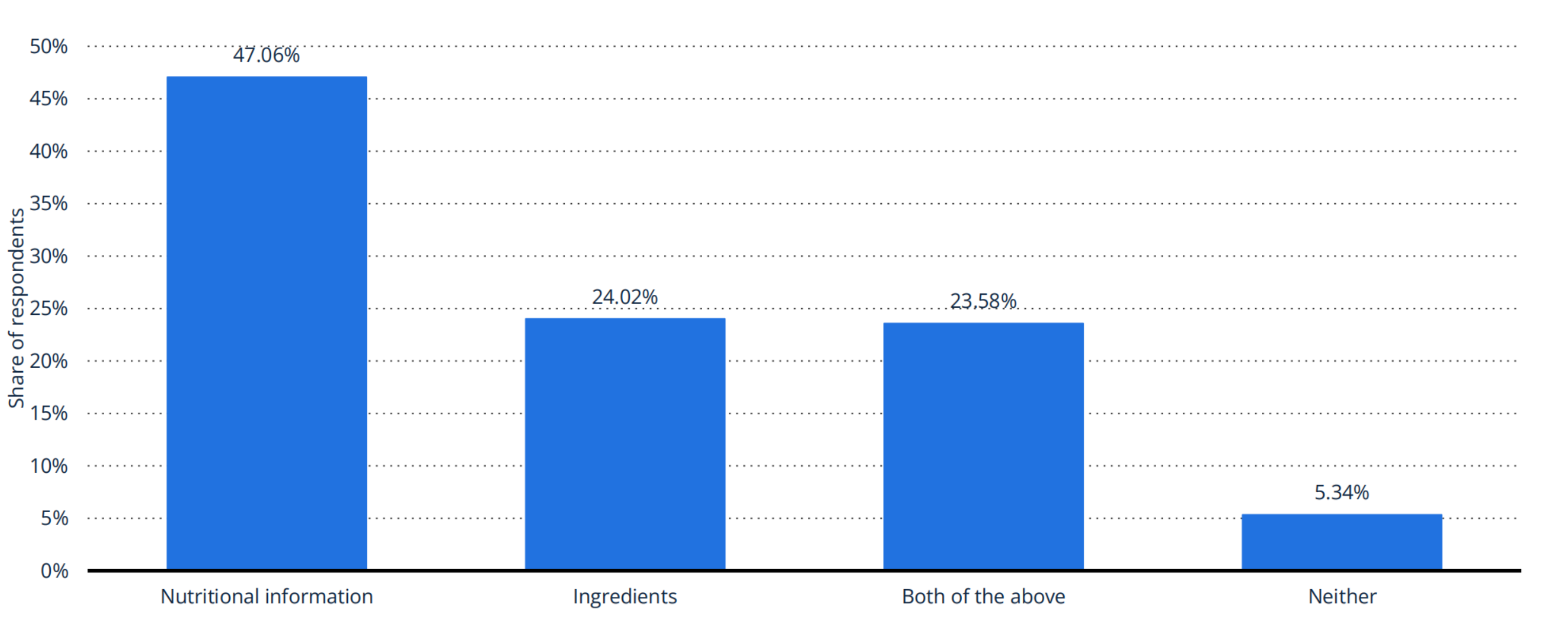
Figure 2.
Would you say that you eat a healthy and balanced diet? (Individual following a healthy and balanced diet in China 2019, by frequency).
Figure 2.
Would you say that you eat a healthy and balanced diet? (Individual following a healthy and balanced diet in China 2019, by frequency).
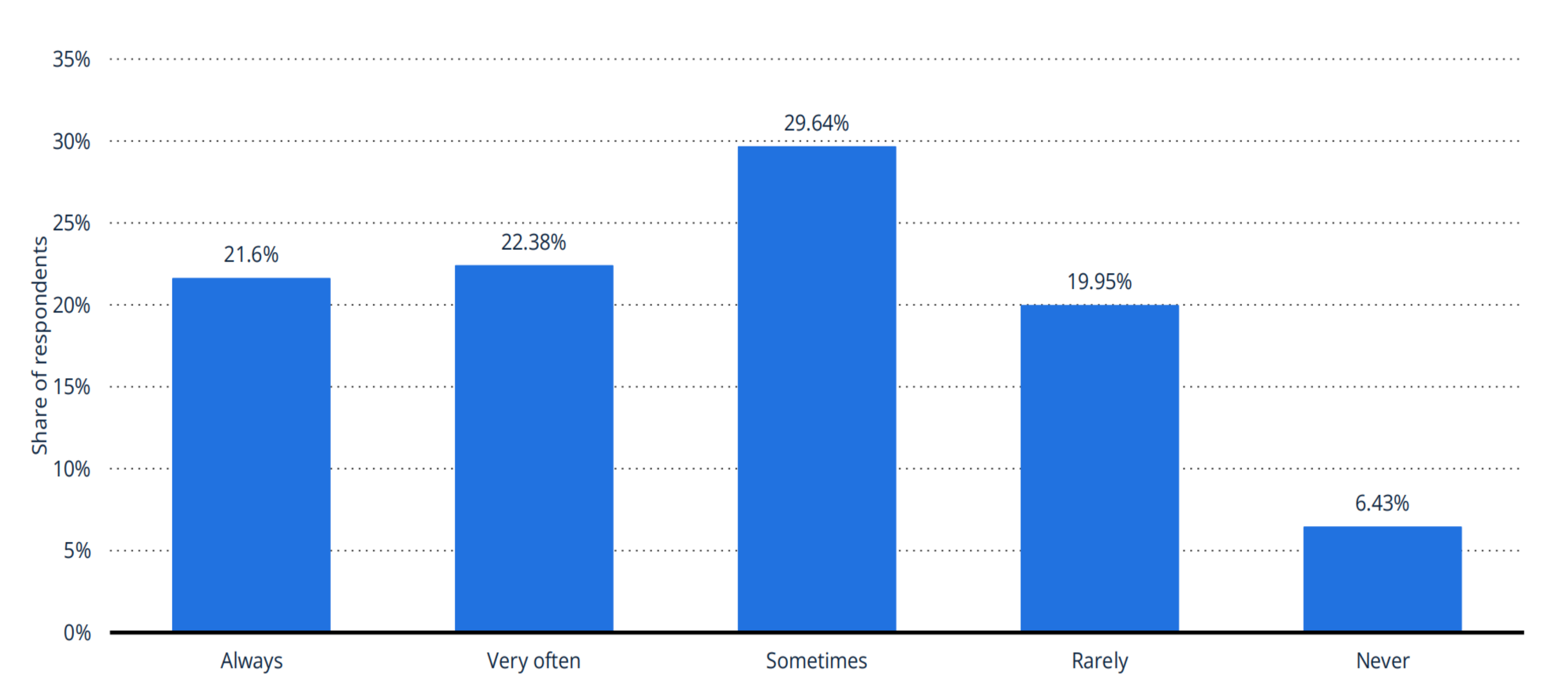
Figure 3.
Vehicle routing problem-solving algorithm.
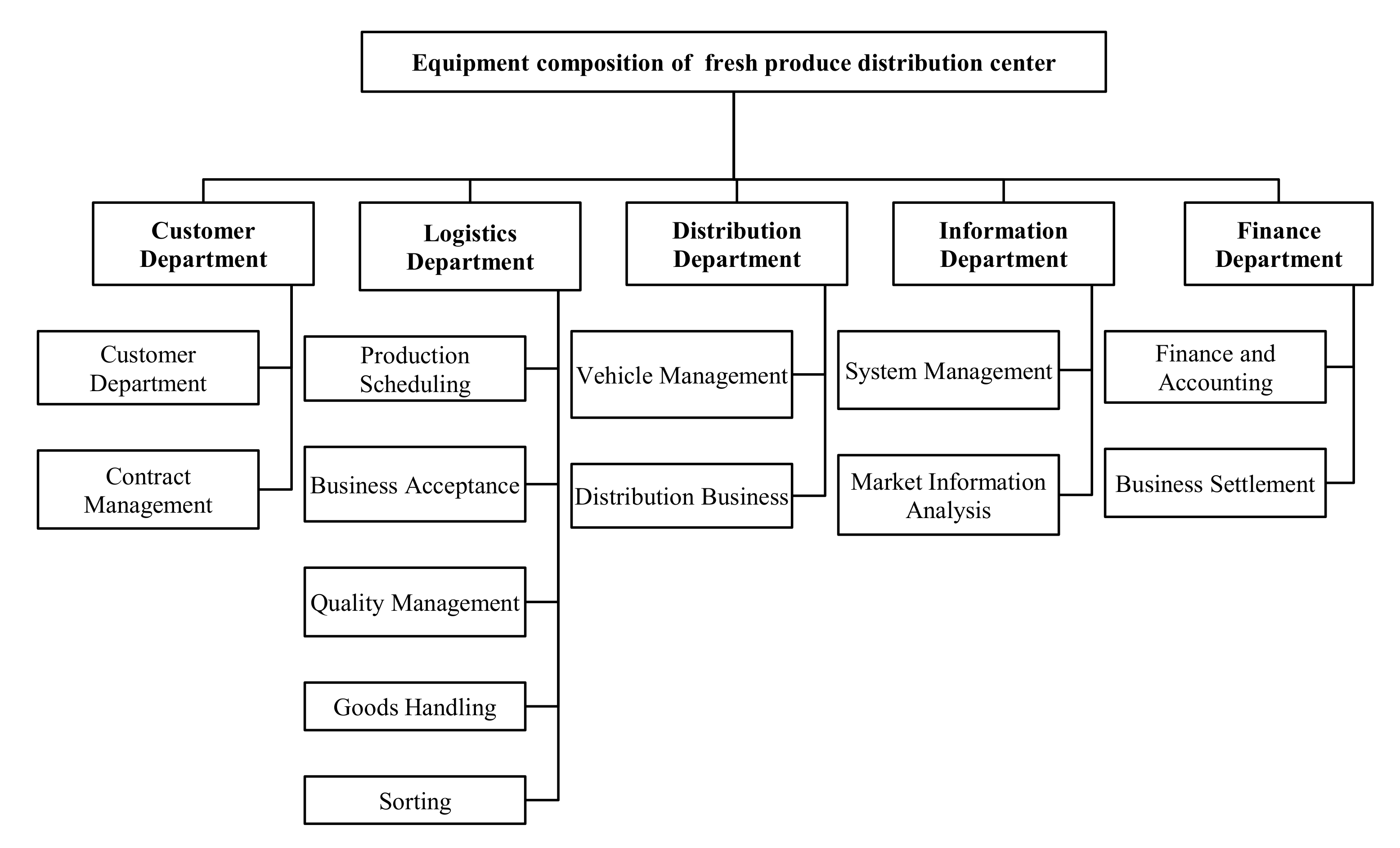
Figure 4.
Organization management system.
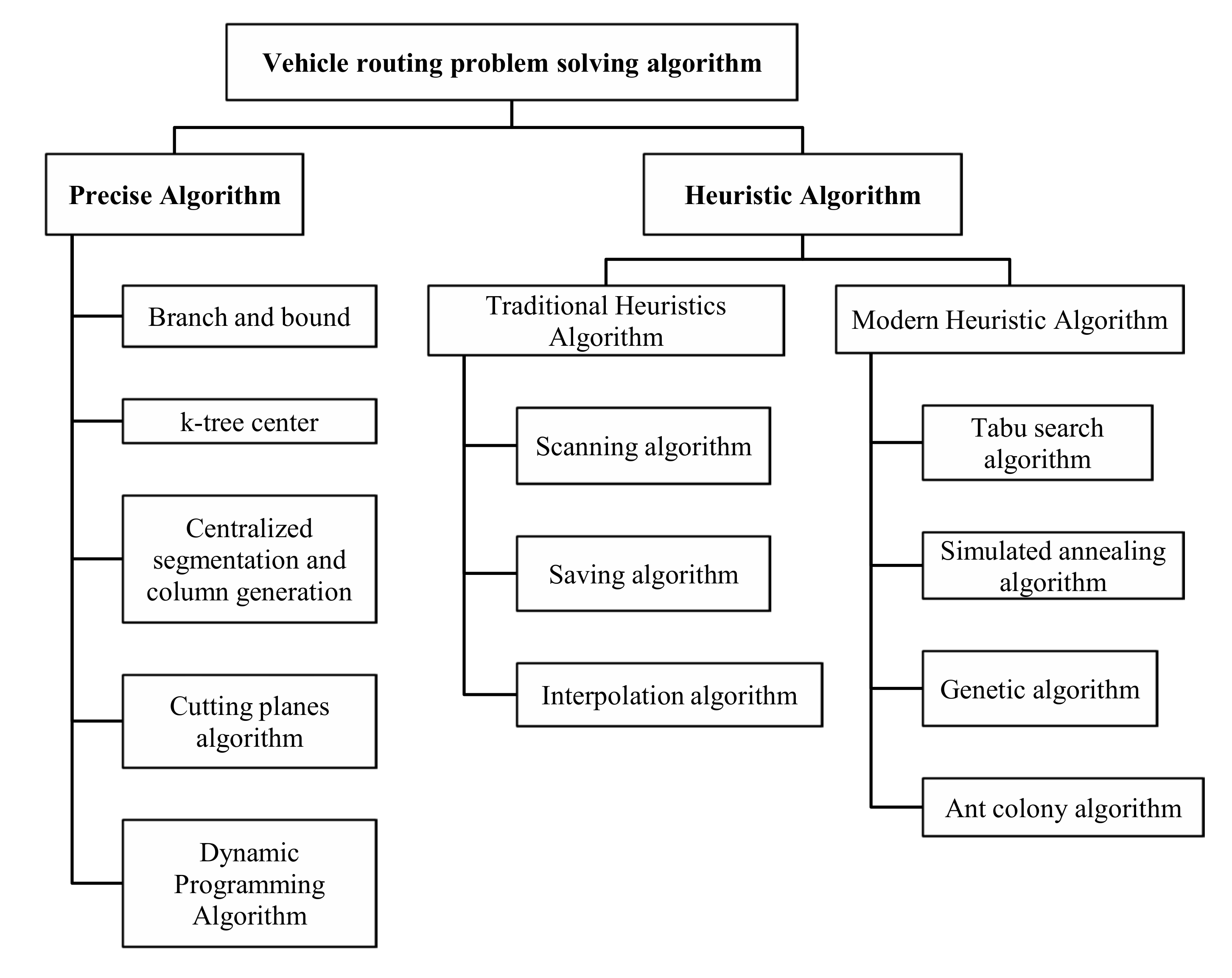
Figure 5.
Equipment composition diagram.
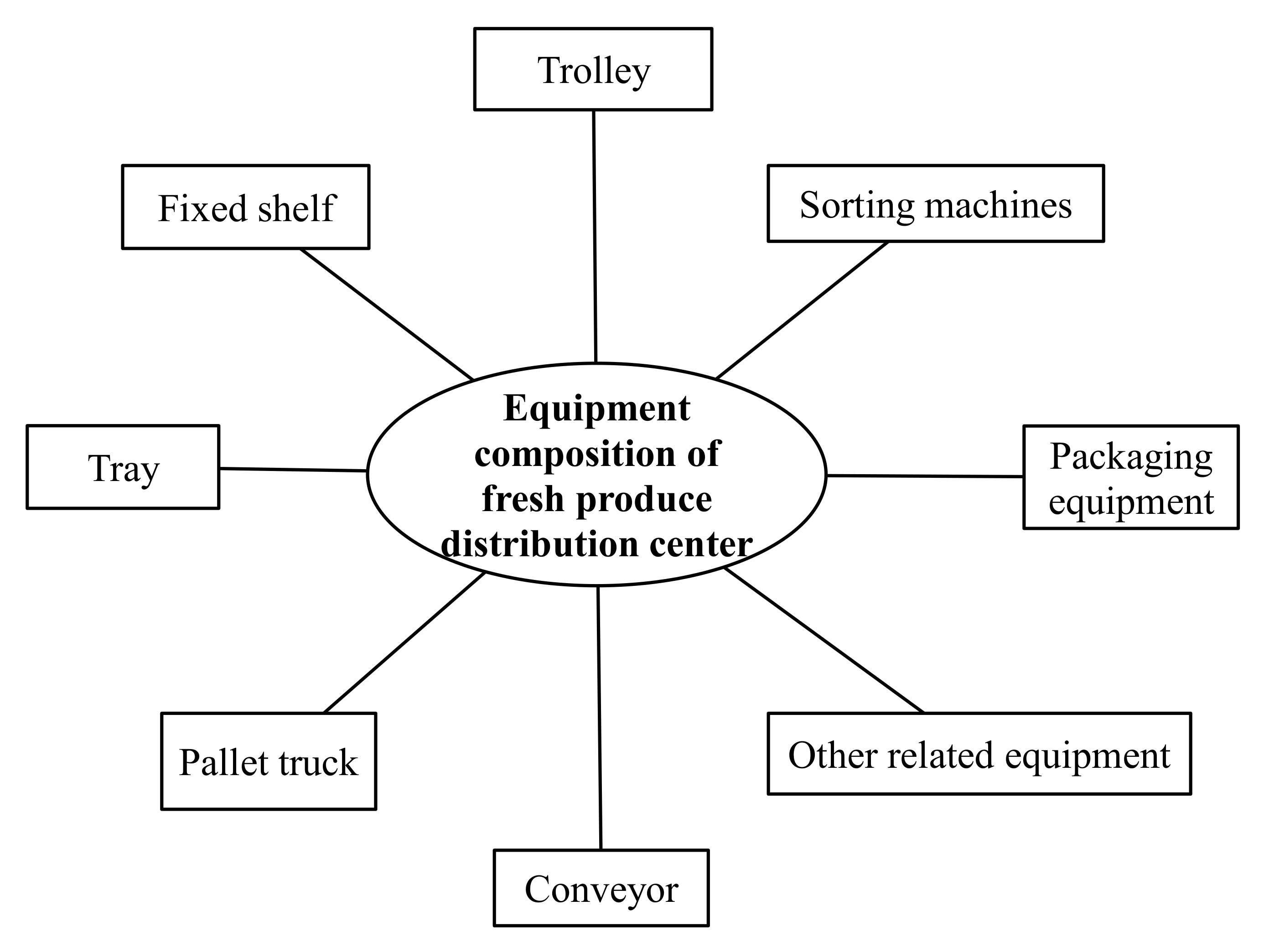
Figure 6.
Penalty cost line chart.
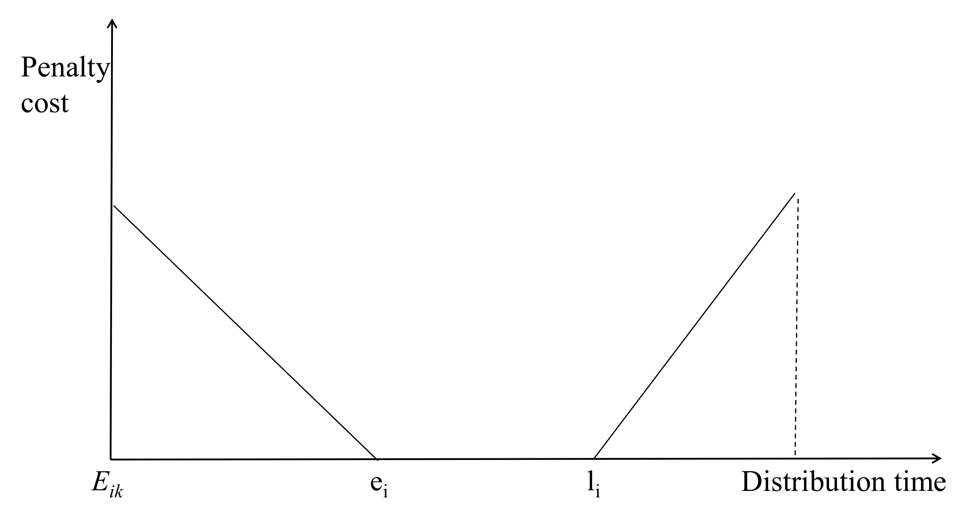
Figure 7.
Customer satisfaction function graph (1).
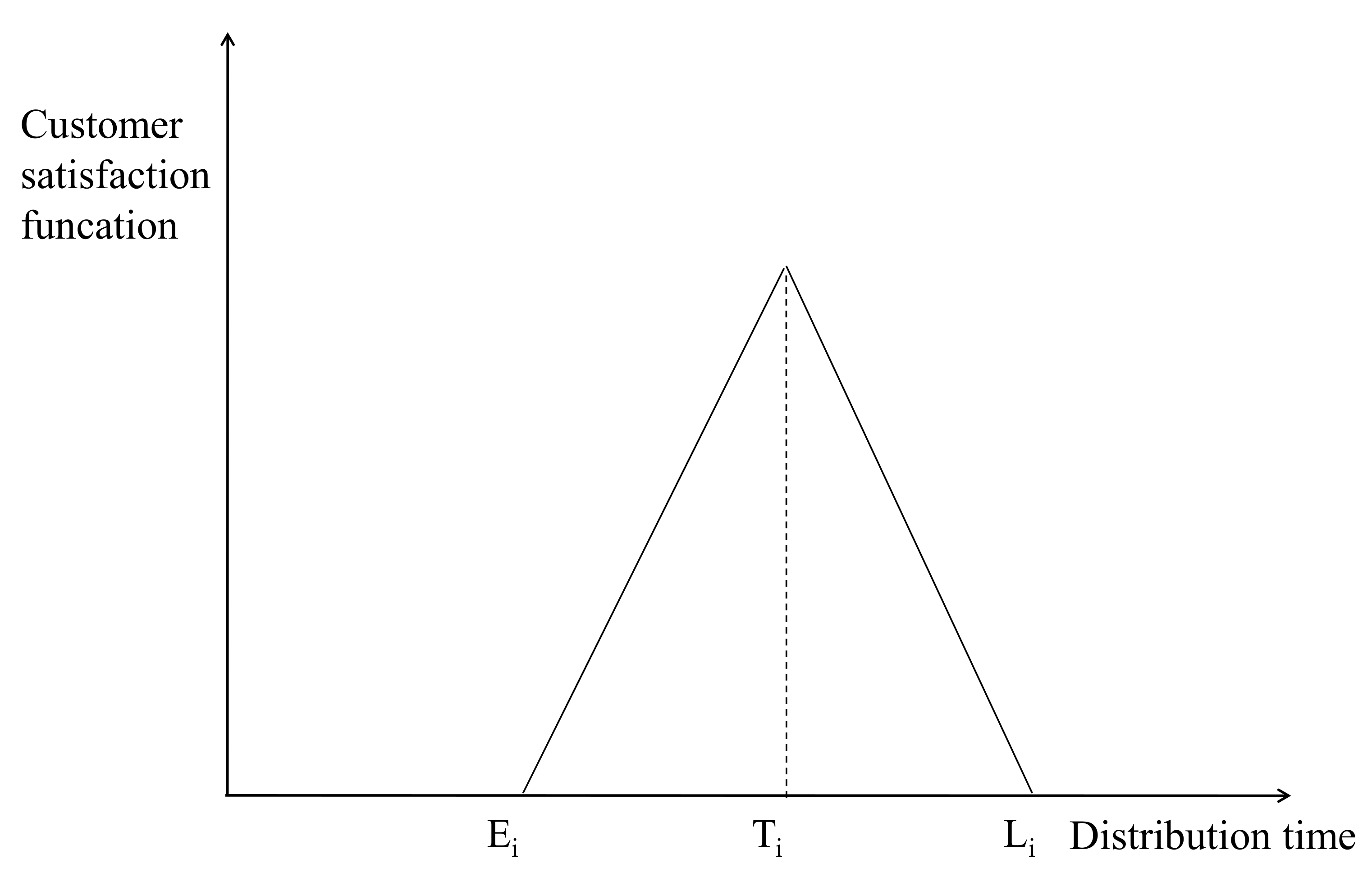
Figure 8.
Customer satisfaction function graph (2).
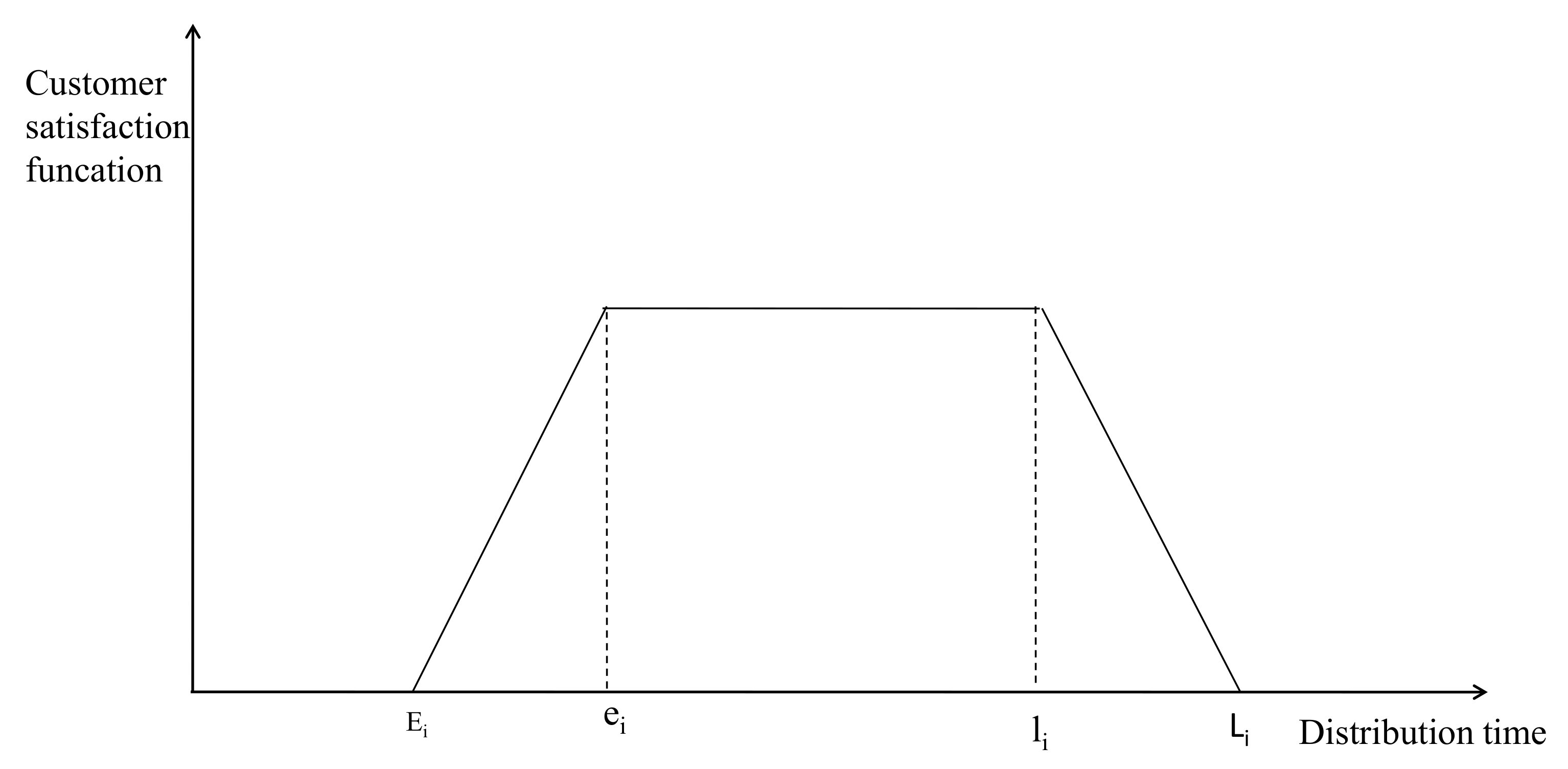
Figure 9.
TheR Distribution center customer points.

Figure 10.
Cost search iteration chart.
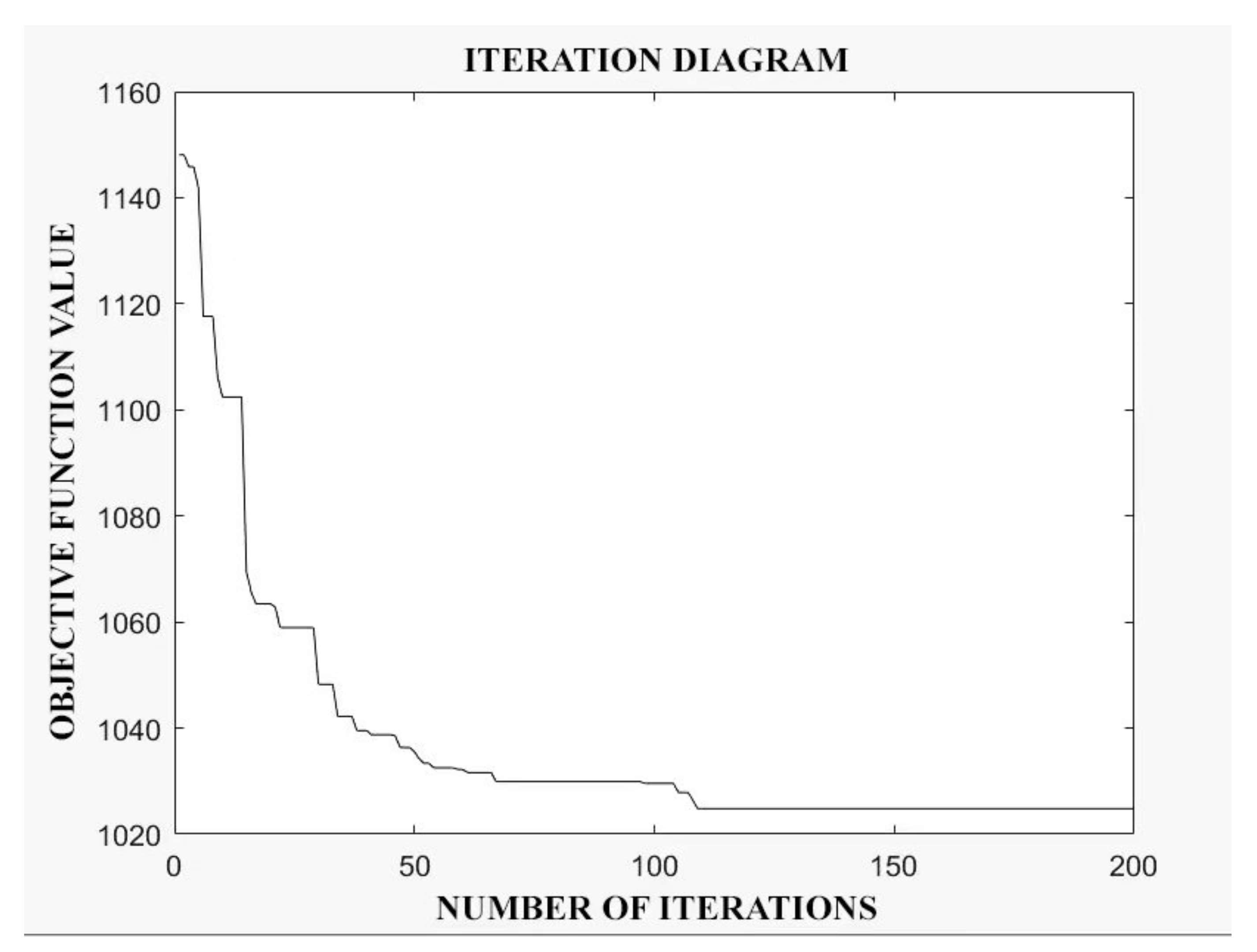
Figure 11.
Optimized path planning diagram.

Table 1.
Classification of Distribution Route Optimization Problems.
| Classification Standards | Type | Definition |
|---|---|---|
| Type of vehicle | Single-type distribution | Delivery by one vehicle type |
| Multi-type distribution | Delivery by multiple vehicle types | |
| Number of distribution centers | Vehicle routing with a single depot | One distribution center |
| Vehicle routing with multiple depots | Multiple distribution centers | |
| Number of optimization targets | Single target | One optimization target |
| Multiple targets | Multiple optimization targets | |
| Time windows | Hard time windows | Delivery within the time window |
| Soft time windows | Deliveries can be made outside the time window, but with penalties. | |
| No time windows | No limitation on delivery time | |
| Fuzzy time windows | Setting a time window that can influence customer satisfaction | |
| Return Restrictions | Open vehicle routing | Vehicles do not need to return to the distribution center. |
| Enclosed vehicle routing | Vehicles need to be returned to the distribution center. | |
| Whether the decision information is certain | Static | Information on distribution environment and demand point conditions is certain. |
| Dynamic | Information on distribution environment and demand point conditions is uncertain. | |
| Vehicle loading | Fully loaded | The load of the vehicle is less than the single demand point requirement. |
| Non-full load | The load of the vehicle is greater than the single demand point needs. |
Table 2.
Model Symbol.
| Symbols | Practical Meanings | Symbols | Practical Meanings |
|---|---|---|---|
| n | The number of vehicles put into the distribution chain. | [ei,li] | Customer i specified deliverable time period. |
| k | The kth vehicle.k∈{1,2,⋯,n} | Ei | The earliest delivery time tolerated by customer i. |
| i, j, p | Distribution center or customer location. | Li | The latest delivery time that can be tolerated by customer i. |
| R | R = {i, j, p|i, j, p = 1,⋯,m} | [Ei,Li] | The delivery time period that can be tolerated by customer i. |
| f1 | Fixed costs incurred per vehicle in the distribution chain. | Ti | Customer i defined time point for satisfactory service. |
| Dij | Miles traveled between customer i and j. | Aik | Actual time of arrival of the kth vehicle at customer i’s location |
| f2 | Transportation cost per unit distance | f3 | Waiting costs incurred per unit of time in case of early arrival |
| Xijk | 0,1 variables, indicating that the kth vehicle completes the delivery operation for customer i,j. | f4 | Delayed costs incurred per unit of time in case of delayed arrival |
| Eik | Earliest time for the kth vehicle to arrive at customer i’s location | Xik | 0,1 variables, indicating that the delivery operation of customer i is completed by the kth vehicle |
| Lik | Latest time for the kth vehicle to arrive at customer i’s location | Qk | Actual load of the kth vehicle |
| [Eik,Lik] | Time period for the arrival of the kth vehicle at customer i’s location | qi | Actual demand of customer i |
| ei | The earliest time that can be delivered as specified by customer i | Q | Maximum load of distribution vehicles |
| li | The latest deliverable time specified by customer i |
Table 3.
Distribution point address and code.
| Name | Address | Code |
|---|---|---|
| R Fresh produce distribution center | No. 1, Yingjun Road, Jinzhou District, Dalian | 0—distribution center |
| Distribution point 1 | No. 10 Xuefu Street, Jinzhou District, Dalian | 1—P1 |
| Distribution point 2 | Huaihe Middle Road, Jinzhou District, Dalian | 2—P2 |
| Distribution point 3 | East Liahe Road and Shuang D1 Street, Jinzhou District, Dalian | 3—P3 |
| Distribution point 4 | Intersection of Dong’an Road and Donghui Street, Jinzhou District, Dalian | 4—P4 |
| Distribution point 5 | No. 50–66, Pengyun Home, Jinzhou District, Dalian | 5—P5 |
| Distribution point 6 | Near Kushan Middle Road, Jinzhou District, Dalian | 6—P6 |
| Distribution point 7 | Near Maqiaozi Street, Jinzhou District, Dalian | 7—P7 |
| Distribution point 8 | No. 19, Tonghui Road, Jinzhou District, Dalian | 8—P8 |
| Distribution point 9 | No. 18, West Liahe Road, Jinzhou District, Dalian | 9—P9 |
| Distribution point 10 | No. 31 Tieshan West Road, Jinzhou District, Dalian | 10—P10 |
| Distribution point 11 | No. 14 Tieshan West Road, Jinzhou District, Dalian | 11—P11 |
| Distribution point 12 | No. 288 Jingang Road, Jinzhou District, Dalian | 12—P12 |
| Distribution point 13 | Intersection of Jingang Road and Longwan Road, Jinzhou District, Dalian | 13—P13 |
Table 4.
Send point data information.
| Node Coordinates | Horizontal Coordinate (Latitude) | Vertical Coordinate (Longitude) | Distance (km) | Demand (t) |
|---|---|---|---|---|
| 1 | 39.106662 | 121.826772 | 10.3 | 0.43 |
| 2 | 39.077017 | 121.856698 | 7.8 | 0.55 |
| 3 | 39.070833 | 121.871083 | 11.5 | 0.26 |
| 4 | 39.046255 | 121.818441 | 7.0 | 0.5 |
| 5 | 39.031466 | 121.813384 | 7.9 | 0.47 |
| 6 | 38.969756 | 121.852591 | 17.5 | 0.70 |
| 7 | 39.054987 | 121.808604 | 5.8 | 0.485 |
| 8 | 39.104574 | 121.840646 | 10.9 | 0.37 |
| 9 | 39.051454 | 121.781714 | 3.7 | 0.44 |
| 10 | 39.075549 | 121.775135 | 2.5 | 0.5 |
| 11 | 39.071659 | 121.765949 | 3.0 | 0.55 |
| 12 | 39.083375 | 121.747865 | 4.2 | 0.45 |
| 13 | 39.082096 | 121.730709 | 4.0 | 0.44 |
Table 5.
Distance table between distribution points.
| Node Label (km) | 1 | 2 | 3 | 4 | 5 | 6 | 7 | 8 | 9 | 10 | 11 | 12 | 13 |
|---|---|---|---|---|---|---|---|---|---|---|---|---|---|
| 1 | 0 | ||||||||||||
| 2 | 5.1 | 0 | |||||||||||
| 3 | 8.6 | 4.8 | 0 | ||||||||||
| 4 | 7.8 | 5.4 | 8.2 | 0 | |||||||||
| 5 | 9.7 | 7.3 | 10.1 | 3.2 | 0 | ||||||||
| 6 | 17.8 | 15.4 | 15.7 | 11.4 | 10.1 | 0 | |||||||
| 7 | 7.8 | 5.4 | 8.2 | 2.6 | 5.1 | 13.2 | 0 | ||||||
| 8 | 7.0 | 4.6 | 5.5 | 9.0 | 11.1 | 19.3 | 8.4 | 0 | |||||
| 9 | 10.5 | 7.7 | 10.4 | 3.8 | 5.1 | 14.4 | 8.7 | 10.7 | 0 | ||||
| 10 | 7.1 | 7.2 | 9.9 | 5.4 | 7.8 | 16 | 3.4 | 8.2 | 4.5 | 0 | |||
| 11 | 8.3 | 7.7 | 10.5 | 5.9 | 8.4 | 16.5 | 4.4 | 9.4 | 5.0 | 1.0 | 0 | ||
| 12 | 10.5 | 10.0 | 12.7 | 8.2 | 10.6 | 18.8 | 6.6 | 16.1 | 7.3 | 3.2 | 2.2 | 0 | |
| 13 | 12.1 | 11.6 | 14.3 | 9.8 | 11.0 | 20.4 | 8.2 | 13.2 | 7.5 | 4.8 | 3.8 | 1.7 | 0 |
Table 6.
Customer best service time window and tolerable time window statistics table.
| Node Coordinates | Optimal Service Time Window [ei,li] | Tolerable Time Window [Ei,Li] | ||
|---|---|---|---|---|
| Earliest Time ei | Latest Time li | Earliest Time Ei | Latest Time Li | |
| 1 | 06.00 | 09.00 | 05.00 | 10.00 |
| 2 | 06.00 | 09.00 | 05.00 | 10.00 |
| 3 | 05.30 | 08.30 | 04.30 | 09.30 |
| 4 | 06.30 | 09.30 | 05.30 | 10.30 |
| 5 | 05.30 | 08.30 | 04.30 | 09.30 |
| 6 | 06.30 | 09.30 | 05.30 | 10.30 |
| 7 | 06.00 | 09.00 | 05.00 | 10.00 |
| 8 | 06.30 | 09.30 | 05.30 | 10.30 |
| 9 | 07.00 | 10.00 | 06.00 | 11.00 |
| 10 | 05.30 | 08.30 | 04.30 | 09.30 |
| 11 | 06.30 | 09.30 | 05.30 | 10.30 |
| 12 | 06.00 | 09.00 | 05.00 | 10.00 |
| 13 | 05.30 | 08.30 | 04.30 | 09.30 |
Table 7.
Other values in the model.
| Parameter | Takes Values |
|---|---|
| Unit vehicle fixed cost (CNY/vehicle) | 150.0 |
| Unit distance transportation cost (CNY/km) | 2.0 |
| Early arrival waiting fee (CNY/h) | 10.0 |
| Delayed arrival delay fee (CNY/h) | 20.0 |
| Vehicle maximum load capacity (t) | 1.5 |
| Average vehicle speed (km/h) | 30.0 |
| Average customer service time (h) | 0.5 |
Table 8.
Genetic algorithm parameter setting.
| Parameter | Initial Population Size | Crossover Probability | Mutation Probability | Maximum Number of Iterations |
|---|---|---|---|---|
| Takes values | 200 | 0.9 | 0.1 | 200 |
Table 9.
Optimized distribution path table.
| Route Number | Driving Path |
|---|---|
| 1 | 0-2-8-1-0 |
| 2 | 0-11-10-0 |
| 3 | 0-3-6-5-0 |
| 4 | 0-7-4-9-0 |
| 5 | 0-13-12-0 |
Table 10.
Distribution path table before optimization.
| Route Number | Driving Path |
|---|---|
| 1 | 0-10-1-0 |
| 2 | 0-3-2-0 |
| 3 | 0-7-8-0 |
| 4 | 0-4-9-0 |
| 5 | 0-5-6-0 |
| 6 | 0-11-12-13-0 |
Table 11.
List of distribution vehicles before optimization.
| Vehicle Number | Order of Visit | Load Capacity (t) | Route (km) | Time (h) | Full Load Rate (%) |
|---|---|---|---|---|---|
| 1 | 0-10-1-0 | 0.93 | 19.9 | 1.66 | 62 |
| 2 | 0-3-2-0 | 0.81 | 24.1 | 1.80 | 54 |
| 3 | 0-7-8-0 | 0.85 | 25.1 | 1.84 | 57 |
| 4 | 0-4-9-0 | 0.94 | 8.2 | 1.27 | 63 |
| 5 | 0-5-6-0 | 1.17 | 35.5 | 2.18 | 78 |
| 6 | 0-11-12-13-0 | 1.44 | 10.9 | 1.86 | 96 |
Table 12.
Optimization of vehicle travel time nodes before.
| Route Number | Time Nodes |
|---|---|
| 1 | 0(05:00)-10(05:05–05:35)-1(05:50–06:20)-0(06:40) |
| 2 | 0(05:00)-3(05:23–05:53)-2(06:03–06:33)-0(06:49) |
| 3 | 0(05:00)-7(05:12–05:42)-8(05:59–06:29)-0(06:51) |
| 4 | 0(05:00)-4(05:14–05:44)-9(05:52–06:22)-0(07:00) |
| 5 | 0(05:00)-5(05:17–05:47)-6(06:07–06:37)-0(07:12) |
| 6 | 0(05:00)-11(05:06–05:36)-12(05:41–06:11)-13(06:15–06:45)-0(06:53) |
Table 13.
Optimize the pre-delivery vehicle cost table.
| Vehicle Number | Fixed Cost (CNY) | Transportation Cost (CNY) | Penalty Cost (CNY) | Total |
|---|---|---|---|---|
| 1 | 150 | 39.8 | 20 | 209.8 |
| 2 | 150 | 48.2 | 10 | 208.2 |
| 3 | 150 | 50.2 | 20 | 220.2 |
| 4 | 150 | 16.4 | 40 | 206.4 |
| 5 | 150 | 71.0 | 20 | 241.0 |
| 6 | 150 | 21.8 | 40 | 211.8 |
Table 14.
List of optimized delivery vehicles.
| Vehicle Number | Order of Visit | Load Capacity (t) | Route (km) | Time (h) | Full Load Rate (%) |
|---|---|---|---|---|---|
| 1 | 0-2-8-1-0 | 1.35 | 29.7 | 2.49 | 90 |
| 2 | 0-11-10-0 | 1.05 | 6.5 | 1.22 | 70 |
| 3 | 0-3-6-5-0 | 1.43 | 45.2 | 3.00 | 95 |
| 4 | 0-7-4-9-0 | 1.42 | 15.9 | 2.03 | 95 |
| 5 | 0-13-12-0 | 0.89 | 9.9 | 1.33 | 60 |
Table 15.
The optimized vehicle travel time node.
| Route Number | Time Nodes |
|---|---|
| 1 | 0(05:00)-2(05:16–05:46)-8(05:56–06:26)-1(06:40–07:10)-0(07:30) |
| 2 | 0(05:00)-11(05:06–05:36)-10(05:38–06:08)-0(06:13) |
| 3 | 0(05:00)-3(05:23–05:53)-6(06:25–06:55)-5(06:15–06:45)-0(07:00) |
| 4 | 0(05:00)-7(05:20–05:50)-4(05:56–06:26)-9(06:34–07:04)-0(07:12) |
| 5 | 0(05:00)-13(05:08–05:38)-12(05:42–06:12)-0(06:20) |
Table 16.
Optimized delivery vehicle cost table.
| Vehicle Number | Fixed Cost (CNY) | Transportation Cost (CNY) | Penalty Cost (CNY) | Total |
|---|---|---|---|---|
| 1 | 150 | 59.4 | 20 | 229.4 |
| 2 | 150 | 13.0 | 20 | 183.0 |
| 3 | 150 | 90.4 | 20 | 260.4 |
| 4 | 150 | 31.8 | 30 | 211.8 |
| 5 | 150 | 19.8 | 20 | 189.8 |
Table 17.
Comparison table of results before and after optimization.
| Before Optimization | After Optimization | Comparison before and after Optimization | |
|---|---|---|---|
| Number of vehicles (vehicles) | 6.0 | 5.0 | −1.0 |
| Fixed cost (CNY) | 900.0 | 750.0 | −150.0 |
| Transportation cost (CNY) | 247.4 | 214.4 | −33.0 |
| Penalty cost (CNY) | 150.0 | 110.0 | −40.0 |
| Distribution cost (CNY) | 1294.4 | 1074.4 | −220.0 |
| Distribution mileage (km) | 123.7 | 107.2 | −16.5 |
| Customer satisfaction (%) | 87.9 | 88.3 | +0.4 |
Publisher’s Note: MDPI stays neutral with regard to jurisdictional claims in published maps and institutional affiliations. |
© 2022 by the authors. Licensee MDPI, Basel, Switzerland. This article is an open access article distributed under the terms and conditions of the Creative Commons Attribution (CC BY) license (https://creativecommons.org/licenses/by/4.0/).
Share and Cite
MDPI and ACS Style
Sun, J.; Jiang, T.; Song, Y.; Guo, H.; Zhang, Y. Research on the Optimization of Fresh Agricultural Products Trade Distribution Path Based on Genetic Algorithm. Agriculture 2022, 12, 1669. https://doi.org/10.3390/agriculture12101669
AMA Style
Sun J, Jiang T, Song Y, Guo H, Zhang Y. Research on the Optimization of Fresh Agricultural Products Trade Distribution Path Based on Genetic Algorithm. Agriculture. 2022; 12(10):1669. https://doi.org/10.3390/agriculture12101669
Chicago/Turabian StyleSun, Jun, Tianhang Jiang, Yufei Song, Hao Guo, and Yushi Zhang. 2022. "Research on the Optimization of Fresh Agricultural Products Trade Distribution Path Based on Genetic Algorithm" Agriculture 12, no. 10: 1669. https://doi.org/10.3390/agriculture12101669
Note that from the first issue of 2016, this journal uses article numbers instead of page numbers. See further details here.