Nighttime Image Dehazing Based on Point Light Sources

Abstract

Images routinely suffer from quality degradation in fog, mist, and other harsh weather conditions. Consequently, image dehazing is an essential and inevitable pre-processing step in computer vision tasks. Image quality enhancement for special scenes, especially nighttime image dehazing is extremely well studied for unmanned driving and nighttime surveillance, while the vast majority of dehazing algorithms in the past were only applicable to daytime conditions. After observing a large number of nighttime images, artificial light sources have replaced the position of the sun in daytime images and the impact of light sources on pixels varies with distance. This paper proposed a novel nighttime dehazing method using the light source influence matrix. The luminosity map can well express the photometric difference value of the picture light source. Then, the light source influence matrix is calculated to divide the image into near light source region and non-near light source region. Using the result of two regions, the two initial transmittances obtained by dark channel prior are fused by edge-preserving filtering. For the atmospheric light term, the initial atmospheric light value is corrected by the light source influence matrix. Finally, the final result is obtained by substituting the atmospheric light model. Theoretical analysis and comparative experiments verify the performance of the proposed image dehazing method. In terms of PSNR, SSIM, and UQI, this method improves 9.4%, 11.2%, and 3.3% over the existed night-time defogging method OSPF. In the future, we will explore the work from static picture dehazing to real-time video stream dehazing detection and will be used in detection on potential applications.

1. Introduction

With the acceleration of industrial modernization, the smoke and dust emitted by factories and the exhaust gas from gasoline combustion are mixed with atmospheric particles to form haze. As a kind of disastrous weather, haze is increasingly common in our daily life. As particles in the atmosphere, haze absorbs and scatters light, which blurs the background of the image captured by the imaging sensor device, significantly reduces the visibility of the scene, and masks the details of image. Image dehazing is of great significance for computer vision tasks [1]. Before images taken on foggy days are input into computer vision algorithms frame (such as object detection [2,3,4,5], scene recognition [6], etc.), it is necessary to preprocess the images to improve the effectiveness of subsequent models. Many practical applications, such as video surveillance, automatic driving, and outdoor vision systems, all need the help of image dehazing technology to improve system effects.

Image dehazing technology [7] can be divided into single-image dehazing and multi-image dehazing. The multi-image dehazing [8] requires numerous additional information inputs. In addition, the scene geometry model used for multi-image dehazing needs large images of the same scene under different weather conditions or different polarization states to be compared and analyzed. This kind of information input limits the application of this method in real life scenes. Therefore, researchers pay more attention to single-image dehazing methods. Single-image dehazing falls into three categories: enhancement-based methods, physical model-based methods, and learning-based methods. Image enhancement aims to emphasize and enhance some feature attributes of foggy images. Tan [9] divides the image into several small blocks, and maximizes the contrast of each small block to remove fog. Bekaert et al. (2012) [10] and Ancuti (2013) [11] introduced fusion-based methods, which fused results, such as white balance, contrast enhancement, etc. Choi et al. (2015) [12] proposed a non-reference perceptual fog density prediction model and enhanced images based on this model. Although image enhancement methods can improve the contrast of foggy images, there is still a lack of physical explanation for the results of dehazing technology.

The physical model approach is mainly based on the atmospheric scattering model [13], which interprets foggy images as a combination of fog-free images and atmospheric lighting. Estimating transmission maps and atmospheric light maps are the two main tasks of physical model-based approaches. For the transmission map, many researchers have proposed their own solutions: dark channel prior estimation [14,15], color attenuation prior estimation [16,17], fog line prior method [18], etc. The learning-based method [19,20,21] is that researchers adjust parameters of neural network through training data to obtain the corresponding dehazing model. Many researchers also combine physical models and learning-based methods to accomplish this task. Zhu et al. [22] reformulated the atmospheric scattering model into a generative adversarial network, where the network model learns atmospheric light and transmittance from the data, and reworked the model to improve the interpretability of the GAN. Huang et al. utilized the haze feature sequence obtained by self-encoding network to calculate the scene transmittance, finally substituted it into atmospheric scattering model to restore the dehazed image. However, deep learning methods require high-quality training data. In addition, some training methods are expensive, requiring the consumption of processors and GPUs.

Almost all of dehazing strategies mentioned above are aimed at daytime. Generally, the sun is the main light source for daytime images, and the overall atmospheric light basically remains constant. Affected by artificial light, such as street lights and car lights, the atmospheric light value at night is not uniform. Therefore, the daytime dehazing algorithms are not necessarily applicable for nighttime images. Furthermore, extensive previous experiments have demonstrated that some well-behaved image dehazing frameworks under daytime conditions cannot be directly applied to nighttime tasks.

According to the analysis of scene conditions, nighttime images have the following characteristics: (1) it is difficult to determine the illumination intensity and range of artificial light sources. If there are many artificial light sources in the image, the pixel values of weaker light sources will also be affected by the strong light sources. Depending on the position of the imaging device, reflected light from objects in the captured image is attenuated differently. (2) In contrast to sunlight, the light emitted by artificial light sources is colored. The color description of an object in the nighttime image is the superposition of the color of itself and the color of the artificial light source.

In view of the above-mentioned characteristics of atmospheric light in foggy scenes at night, some researchers take advantage of illumination compensation and color correction to modify spatially varying illumination. Zhang et al. [23] used the enhanced light intensity to balance illumination and corrected the color of incident light to estimate accurate ambient light; Pei et al. [24] improved the dark channel prior to better adapt to nighttime dehazing tasks. In order to enhance the effect, they used color shift and local contrast correction. Though this method produces results with lower contrast and lower brightness overall; Li et al. [25] proposed a relatively smooth constrained layering algorithm to remove the glow effect; based on the Retinex theory [26], Yu et al. [27] estimated the ambient illumination by channel differential guided filtering method, and they used the dark channel prior and the bright channel combination to evaluate the dehazing transmission map; paying attention to preserving the details of the fine structure area, Yang et al. [28] decomposed the image into luminous image and non-luminous night image. They calculated the value of the atmospheric light and dark channels of each pixel in the non-luminous night image based on the superpixel method. Then, the transmission map is decomposed from fog-free image through the weighted guided image filter. All the above methods have achieved good results. However, past methods basically have some defects, such as color distortion, serious loss of texture details, and insufficient effect. Therefore, the task of dehazing nighttime images requires model reconstruction. Based on He’s dark channel theory dehazing algorithm (DCP) [14], this paper proposes an improved nighttime dehazing algorithm for the influence matrix of artificial light sources. According to the light intensity of light source points, we filter the light source through the photometric map and obtain the corresponding light source influence matrix. The transmittance near the light source can be adaptively adjusted to reduce the glow effect near the light source by the light intensity matrix. The experimental results demonstrate that the method has great dehazing effect and detail retention at night, and the color cast problem of the restored image is also improved. Our main contributions are as follows:

• The light source influence matrix is proposed to adaptively modify the transmittance near the artificial light source, so as to improve the dehazing task.
• To enhance the detail of image, we used an edge filter to fuse the transmittance of the near and far light source areas. Furthermore, we used MRP to make the image more colorful.
• For different fog concentration scenes, a bias coefficient is introduced to make the defogging algorithm suitable for dense fog scenes.

The paper is organized as follows: Section 2 reviews the related work. The detailed model and the proposed framework are presented in Section 3. The experiment results and the corresponding analyses are demonstrated in Section 4. Finally, we conclude in Section 5.

2. Related Work

The light will come into contact with suspended particles in the atmosphere during its propagation process, and some of the light will be scattered by the particles, so the light received by the imaging device will be weaker [29]. In 1976, John Wiley et al. [13] proposed that transmission light of the target would be attenuated by scattering, and the transmission device will receive not only the reflected light from the target but also a layer of atmospheric scattered light. Srinivasa G. Narasimhan et al. [30] constructed a method to recover scenes for foggy days with low visibility by visual performance under different weather conditions. McCartney [13] developed an atmospheric scattering model based on the Mie scattering theory, and the expression of the pixel value received by the device is expressed by the following equation:

$$I_x=J_x{t}_x+A(1-t_x)$$

(1)

where x represents the position of the pixel in the image, $I_x$ represents the foggy image, $J_x$ represents the fog-free image, $t_x$ represents the transmission at the position of x in the image, and A represents the atmospheric light value of the image. This model divides the light received by the device into two parts. The first part represents the target reflected light, which means that the reflected light is directly transmitted to the device through the absorption and scattering of airborne particles, also known as the direct attenuation term of incident light; the other part is that the ambient light (mainly including direct sunlight, atmospheric diffuse light, and ground reflected light), which will also be attenuated by the action of the medium in the air.

Many daytime physical model dehazing methods and some nighttime dehazing methods have been designed based on this model. The most typical one is the dark channel dehazing algorithm (DCP), which takes into account the global uniformity of atmospheric light in the daytime environment and can recover satisfactory images of the scene. He et al. [14] studied many fog-free images and found that at least one channel of the non-sky color block of the fog-free image contains very low-intensity pixels, and this color channel is called the dark channel. Ideally, the dark channel of a clear image is approximately zero and is mathematically represented as follows:

$$J_x^{dark}=\underset{y\in \mathsf{\Omega }\left(x\right)}{min}(\underset{c\in \{r,g,b\}}{min}{J}_x^c)\approx 0$$

(2)

However, in foggy images, air light causes the intensity of the color block pixels in these dark channels to increase. Therefore, during the process of recovery, it is necessary to adjust the light transmittance and the atmospheric light value to make the image clear. The author in [14] takes the average value of the first 0.1% pixels of illumination in the dark channel as the atmospheric light value, which is expressed by $A^c,c\in \{r,g,b\}$. The transmittance is estimated from the atmospheric light value, which is mathematically expressed as:

$$t_y=1-\omega \underset{y\in \mathsf{\Omega }\left(x\right)}{min}(\underset{c\in \{r,g,b\}}{min}\frac{I_y^c}{A^c})$$

(3)

Among them, $\omega$ is the introduction parameter which represents the concentration of fog. $t_y$ is the transmission at the position of y in the image, where the position y is a point belonging to the set of light sources $\mathsf{\Omega }\left(x\right)$. $A^c$ means atmospheric light values in the channel c. $I_y^c$ means pixel value at the position of y in the channel c. The image obtained in this way will have a block effect. To solve the above problem, He et al. [14] proposed a soft-matting algorithm to correct the initial transmission map. Finally, the atmospheric light value and transmission map are brought into Equation (1) to obtain the final restored image:

$$J_x=\frac{I_x-A}{t}+A$$

(4)

However, in night scenes, the atmospheric ambient light is susceptible to nighttime lighting [31]. The local maximum intensity of each color channel in the image is mainly provided by artificial light source, so it is inaccurate to use global atmospheric light values to preserve the color characteristic of nighttime images. Therefore, we can reduce the attention on ambient light and directly estimate the ambient illumination and transmittance to recover foggy images. Most of the light radiated by point-like artificial sources varies smoothly in space, except for some sudden changes between bright and dark areas due to shading. In the estimation of ambient illumination, it is necessary to use light intensity normalization and maintain the color component of the artificial light source. Many researchers have analyzed the night scenes and reworked the atmospheric imaging model, as shown in the

Table 1. Related work of dehazing algorithms.

Year	Title	Author	Methods
2011	Single Image Haze Removal Using Dark Channel Prior	He et al. [14]	The dehazing model is simplified by the dark channel prior, and the image dehazing problem is transformed into a matting problem.
2015	Nighttime Haze Removal with Glow and Multiple Light Colors	Li et al. [25]	A night-time halo term is added to the atmospheric lighting model to eliminate the halo effect.
2016	Night-time dehazing by fusion	Ancuti C et al. [33]	Atmospheric light terms for image blocks are estimated using a Laplace pyramid decomposition of the input multiscale image block and a weight map.
2017	Fast Haze Removal for Nighttime Image Using Maximum Reflectance Prior.	Zhang et al. [32]	This article proposes the maximum reflection prior (MRP) method to estimate atmospheric light maps.
2018	Nighttime Image Dehazing Based on Low-Pass Filtering and Joint Optimization of Multi-Feature	Yang et al. [34]	The article uses low-pass filtering to estimate ambient light and use ambient light to predict nighttime transmittance.
2020	Nighttime Dehazing with a Synthetic Benchmark	Zhang et al. [35]	The article proposes an optimal scale based maximum reflectance prioritization algorithm (OSFD) on the basis of MRP.

. Zhang et al. [32] splits the atmospheric light value A in Equation (1) into $L_x{\eta }_x$, which is mathematically represented as:

$$I_x=J_x{t}_x{\eta }_x+L_x{\eta }_x\left(1-t_x\right)$$

(5)

where $L_x$ represents the ambient illumination, and ${\eta }_x$ represents the environmental color coefficient. Although the improved model is effective in the nighttime defogging task, it still can not remove the halo effect from the nighttime images.

For removing the above halo effect, Li et al. [25] suggested adding a nighttime halo term to the original equation:

$$I_x=J_x{t}_x+A\left(1-t_x\right)+A_x\ast APSF$$

(6)

The atmospheric point spread function is expressed as a halo term in the proposed model, and it decays with increasing depth of field. The halo term can represent the halo characteristics of the image, and the new proposed model can estimate the atmospheric light pixel by pixel, so that the halo can be removed from the image more accurately. Nevertheless, it should be noted that some noise in the recovered image is amplified and some color artifacts are generated around the light source.

Zhang et al. [32] observed that each color channel of fog-free images contains some high-intensity pixels. For nighttime images, the high-intensity pixels of their color channels are all contributed by artificial ambient lighting. Based on these observed phenomena, the authors put forward the maximum reflection prior (MRP) to estimate the atmospheric light map. Due to the influence of the color of the artificial light source, the maximum reflectance map of the nighttime image is mathematically expressed as:

$$\begin{array}{cc}\hfill M_{\mathsf{\Omega }\left(x\right)}^c = \underset{x\in \mathsf{\Omega }\left(y\right)}{max}{I}_x^c& =\underset{x\in \mathsf{\Omega }\left(y\right)}{max}{R}_x^c(L_{\mathsf{\Omega }\left(y\right)}{\eta }_{\mathsf{\Omega }\left(y\right)}^c{t}_{\mathsf{\Omega }\left(y\right)})\hfill \\ \hfill & +L_{\mathsf{\Omega }\left(y\right)}{\eta }_{\mathsf{\Omega }\left(y\right)}^c(1-t_{\mathsf{\Omega }\left(y\right)})\hfill \end{array}$$

(7)

Under the action of light, the maximum reflectance is approximated as 1:

$$\underset{x\in \mathsf{\Omega }\left(y\right)}{max}{R}_x^c\approx 1$$

(8)

$$M_{\mathsf{\Omega }\left(x\right)}^c=L_{\mathsf{\Omega }\left(y\right)}{\eta }_{\mathsf{\Omega }\left(y\right)}^c\to {\eta }_{\mathsf{\Omega }\left(y\right)}^c=\frac{M_{\mathsf{\Omega }\left(x\right)}^c}{L_{\mathsf{\Omega }\left(y\right)}}$$

(9)

$$L_{\mathsf{\Omega }\left(y\right)}=\underset{c\in \{r,g,b\}}{max}(\underset{x\in \mathsf{\Omega }\left(y\right)}{max}\widetilde{I_x^c})$$

(10)

In nighttime images, the color channel of the glow part of the light source has a high-intensity value, and MRP can be used to improve the halo around the light source to some extent. The prior models, however, are built based on clear daytime image characteristics, which in some cases are different from the nighttime image characteristics. The fog-free image output with MRP alone will be distorted.

On the basis of MRP, Zhang et al. [35] proposed the Optimal Scale-Based Maximum Reflectance Prior algorithm (OSFD), which considers the maximum reflectance as the probability of a pixel block that completely reflects the incident light in all frequency ranges. Moreover, color correction and defogging are separated and solved sequentially. In addition, the extinction Laplace matrix in the MRP method is replaced by the maximum value of the light intensity in all channels as a way to facilitate the calculation of the light intensity normalization. To reduce the halo effect and retain details, Ancuti C et al. [33] were inspired by the dark channel algorithm to assign higher weights to high-contrast image blocks, and finally used the Laplace pyramid decomposition of the input multi-scale image blocks and weight maps to estimate the atmospheric light terms of the image blocks. A new model for imaging nighttime fog images containing artificial light sources was developed by Yang et al. [34] by deeply analyzing the imaging pattern of nighttime fog images. The ambient light is estimated using low-pass filtering, followed by the prediction of the night scene transmittance using ambient light, and, finally, the histogram matching method is used to color correct the result.

3. Proposed Method

3.1. Problem Analysis

Firstly, the illumination of the light source is uneven. In the nighttime environment, the illumination intensity of the artificial light source is much greater than that of the ambient light, resulting in excessive illumination in the area close to the light source and insufficient illumination in the area far away from the light source, which is why the illumination of the image we see is uneven. Accordingly, the non-constant atmospheric light value plays a significant role in nighttime image dehazing.

Secondly, the color shift of the light source. The intensity of artificial light sources is not like sunlight in the daytime. The color of the light source determines the naturalness of scene objects in the image, and the color of the light source will also affect the final dehazing effect.

Third, the details of the image after dehazing. Since the whole image is in a night scene, the lack of brightness will lead to high noise and serious loss of image details after dehazing. However, if the exposure of the entire image is simply increased, the glow portion will also increase.

3.2. Overview of Algorithm

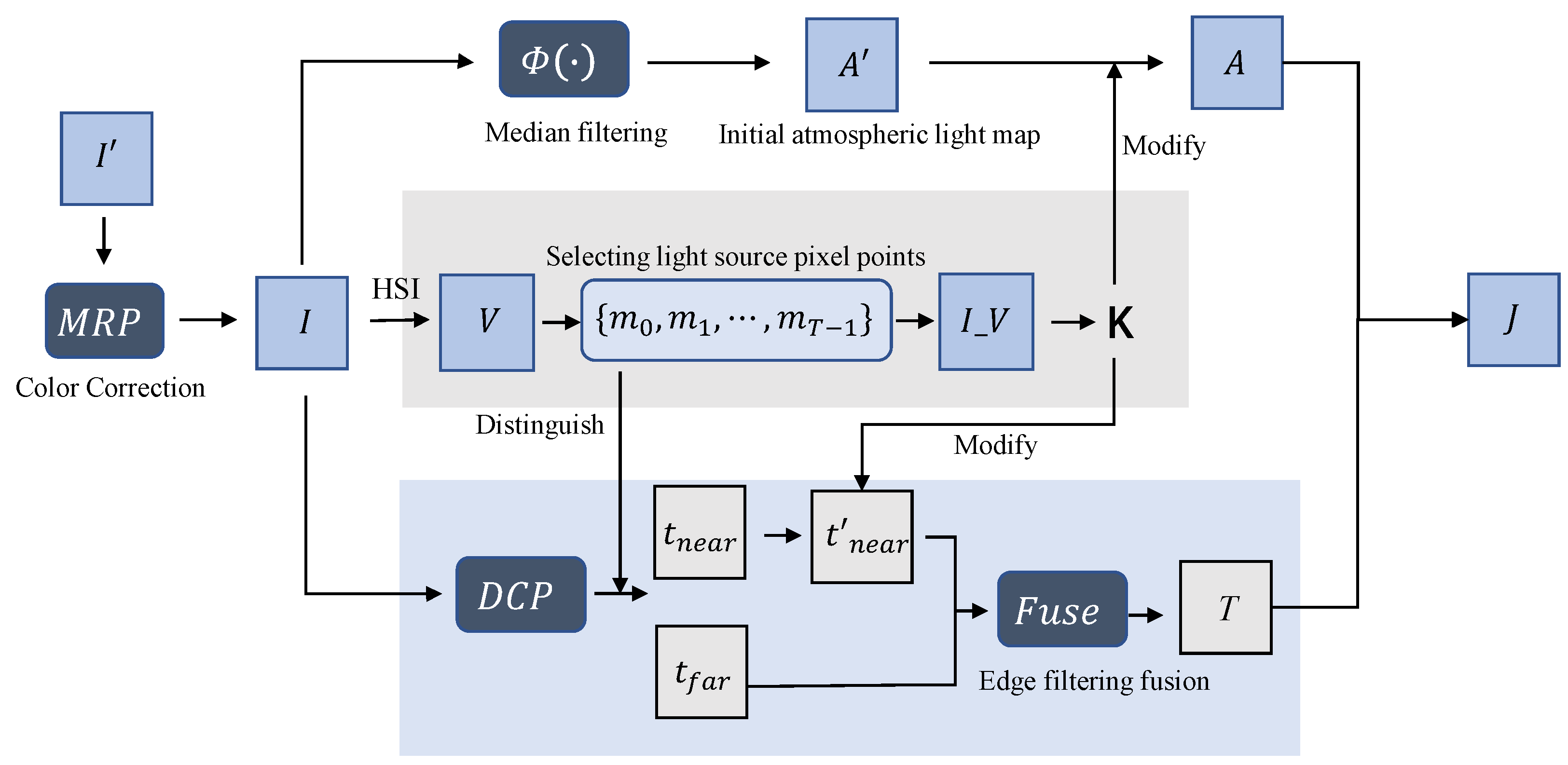
In order to solve the problems of serious texture loss and poor dehazing effect in the nighttime dehazing algorithm, this paper proposes a nighttime dehazing method based on the light source influence matrix. The algorithm flow is shown in Algorithm 1. As illustrated in Figure 1, the whole algorithm consists of a pre-processing section (Color Correction), a section of calculating light source influence matrix, and a dehazing section.

Color Correction: The color of the artificial light source in the night scene has a certain influence on the reflected light of the object. It is necessary to perform color correction on the image at first to prevent color distortion of the image after dehazing. Therefore, the first step is to correct the color shift of the image through the maximum reflection prior algorithm, so as to maintain the color balance of the image and enhance the details of the image.

Light Source Influence Matrix: The low-frequency component is extracted from the image through a mid-pass filter, and the initial atmospheric light value is calculated with the low-frequency component. Then the image is transferred to the HSI space to extract the photometric map. According to the photometric map, the artificial light source pixels are filtered out and the corresponding influence matrix is calculated. After superposition, the final matrix is obtained.

Nighttime Dehaze: Using the light source influence matrix and introducing the adaptive atmospheric light deviation coefficient, the atmospheric light value near the light source area is corrected. The initial transmittance of the two regions is estimated separately from the dark channel method and then refined to fuse the boundary parts of the two regions. Among them, the transmittance of the near-source region is modified and adjusted using the edge-preserving filtering method. Finally, the dehazing image is obtained by optimizing the atmospheric light value, transmittance and the light source influence matrix.

Algorithm 1: Nighttime dehazing algorithm

Data: $I_0$

Result: J

1  Color Correction:

2  $I\leftarrow MRP\left(I_0\right)$

3  Light Source Influence Matrix:

4  calculate the matrix K according to Algorithm 2

5  Parameter Estimation:

6  $A\leftarrow \mathsf{\Phi }\left(I\right)$

7  classify A according to Equation (15)

8  calculate the initial transmittance map $t_{near}$ and $t_{far}$ according to Equation (16)

9  $t\leftarrow Fuse(t_{near},t_{far})$

10  Nighttime Dehaze:

11  synthesize J according to Equation (21)

3.3. Light Source Influence Matrix

According to the MRP theory, the atmospheric light value is replaced by the illumination of artificial light source. As the distance increases, the attenuation of light decreases. The pixels near the light source are more affected by the light source, while the pixels far from the light source are less affected by the light source.

3.3.1. Judging the Near and Far Light Source Area

Convert the image to HSI space, and extract the photometric map of the image. Fully considering nighttime conditions, we default the brightness of artificial light sources to a great extent. The average value of the pixels in the top 0.5% of the photometric value is selected as the light source candidate threshold $C_{max}$. In the photometric map, filter out the light source pixel points whose photometric values are greater than or equal to the threshold value. Keep the light source pixel points in the photometric map to obtain the light source map, and define the pixel blocks in the top 2% of the photometric value as the near light source region $\mathsf{\Omega }$.

3.3.2. Create Light Influence Matrix

According to the T light source pixel points in the light source map, number each light source pixel point in descending of the photometric value $\left\{m_0,m_1,\cdots ,m_{T-1}\right\}$, and calculate the influence matrix for each light source:

$$k_i=\frac{lg\left(1+C_i\right)}{lg\left(1+C_{max}\right)}\ast \frac{C_i}{\left|d_{i,m}\right|}$$

(11)

$$K=\frac{1}{T}\sum _{j=0}^{T-1}{k}_j$$

(12)

The normalized light source influence matrix is closer to 1 in the near light source area $K_i$; When the pixel is closer to the light source, $K_i$ is higher; when the pixel is farther from the light source, influence value corresponding to the pixel is lower. For calculating the light source influence matrix, we summarize the algorithm flow in Algorithm 2.

Algorithm 2: Light influence matrix

3.4. Night-Time Dehaze

3.4.1. Estimating Atmospheric Light

According to the Retinex theory, the modified

$$I_i^{\lambda }=L_i^{\lambda }{R}_i^{\lambda }{t}_i^{\lambda }+A_i^{\lambda }\left(1-t_i\right)$$

(13)

where $R_i^{\lambda }$ is a high-frequency component, the rest of items have the characteristics of smooth change, which belong to low-frequency components. When the pixel position i is far away from the light source, it is less affected by the artificial light source. After processing the image with a low-pass filter, the low-frequency components can be obtained to estimate the ambient light:

$$\mathsf{\Phi }\left(I_i^{\lambda }\right)={\left(I_i^{\lambda }\right)}_L\approx L_i^{\lambda }{t}_i^{\lambda }+A_i^{\lambda }\left(1-t_i\right)$$

(14)

where $\mathsf{\Phi }\left(·\right)$ represents low pass filter, ${\left(I_i^{\lambda }\right)}_L$ represents low frequency components of the image. At the near light source, considering the large deviation of the atmospheric light from the near light source, the influence of the artificial light source far exceeds the surrounding environment.

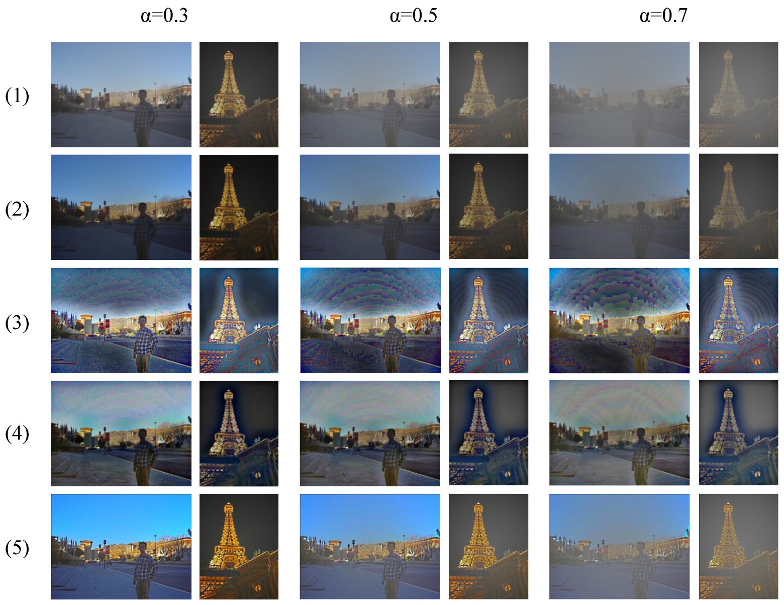
Since the ambient light will be low after superimposing the influence value of the light source, which will affect the subsequent dehazing effect, the atmospheric light deviation coefficient $A_0$ is introduced to modify the atmospheric light value ${\overline{A}}_i^{\lambda }$ near the light source:

$$A_i^{\lambda }=\left\{\begin{array}{c}{\overline{A}}_i^{\lambda }+A_0,i\in \mathsf{\Omega }\hfill \\ {\overline{A}}_i^{\lambda },i\notin \mathsf{\Omega }\hfill \end{array}\right.$$

(15)

It has been verified by a large number of experiments that the dehazing effect of $A_0$ in the range of 0.1–0.16 is better.

3.4.2. Estimating Transmittance

We will use different transmittance estimation methods according to different regions, and obtain their respective transmittances in the near light source area and the non-near light source area. According to the two fusion and refinement, we can obtain the final transmittance.

• Non-near light source area. It is less affected by artificial light sources, and the transmittance of the dark channel prior is superior, so we use the DCP method to estimate it:

  $$t_i=1-w\underset{j\notin \mathsf{\Omega }}{min}\left[min\frac{I^c\left(j\right)}{A^c}\right]$$

  (16)
• Near light source area.
  Due to the influence of the halo effect caused by the transmittance of the dark channel, we propose to re-optimize the transmittance to accurately estimate the transmittance and reduce the Halo effect. $S_i$ is assumed to be the minimum value of a channel in the near light source area, and since the transmittance is continuous in the local area of the image and suddenly changed at a depth of field, the calculation is converted into finding the maximum transmittance:

  $$argmax\int {t-\lambda ∥\nabla t∥}^2$$

  (17)

  $$0<t_{i\in \mathsf{\Omega }}<S_i$$

  (18)

  where $\lambda$ represents the smoothness of the optimized transmittance. In addition, use edge-preserving filtering on the transmittance to make it have the same gradient information as the original image.
• Transmittance Fusion.

  $$t=w_i{t}_{i\in \mathsf{\Omega }}+t_{i\notin \mathsf{\Omega }}$$

  (19)
  $w_i$ is the adjustment correction coefficient.

  $$w_i=\frac{max\left(K_i,t_i\right)}{t_i}+\alpha$$

  (20)
  $\alpha$ is the fog-free image is the adjustment correction coefficient

  $$J_i=\frac{I_i^{\lambda }-A_i^{\lambda }·max\left(K_i,1-t_i\right)}{\max \left(t_i,K_i\right)}$$

  (21)
  In this paper, the transmittance is corrected by defining the near and non-near light source area and fusing the transmittance of the area to solve the halo phenomenon near the light source.

4. Experiment

4.1. Experimental Settings

In order to verify the reliability and validity of the method proposed in this paper. In this experiment, the algorithm programming is performed under Matlab2016b, and the hardware environment of the simulation experiment is i7-10750H, 2.60 GHz, 16 G RAM.

During the experiment, the diameter of the low-pass filter window is 0.06 × min(h, l), h and l are the numbers of pixels in the row and column in the image, respectively. $A_0$ was set to 0.02$\lambda$ was set to 0.1. In order to ensure the effectiveness of the algorithm at night, the dataset used in the experiment is NHRW, which is 150 real nighttime foggy images selected from 3000 images [25,32], and the scenes include urban night scenes, roads, riversides, parks, and other scenes.

4.2. Main Results

In order to verify the universality of the algorithm, foggy images in various environments (city, road, riverside, park) are selected for experiments, and 150 real nighttime foggy scene images are used in the dataset for experiments and evaluation. The selected comparison algorithms include DCP [14], NDIM [25], and OSFD [35]. Through experimental comparison, the experimental results are analyzed and evaluated from both subjective and objective aspects.

As shown in

Table 2. The difference between proposed method and DCP.

Method	Atmospheric Light Values	Transmittance	Applicable Condition
DCP	Takes the maximum value of the first 0.1% of pixels of the image	dark channel prior	Daytime
Proposed method	Median filter	the transmittance of the near light source is corrected by the light source influence matrix	Nighttime

, We compare the differences between the proposed method and DCP in terms of the way to calculate atmospheric light and transmittance. For the atmospheric light value, DCP selects the first 0.1% of the pixel values in the dark channel of the image and then chooses the brightest of these values as the constant atmospheric light value. This method may cause the defogged image to be too light near the light source. Our method calculates the atmospheric light value by making the image through the median filter directly. For transmittance, the proposed method corrects the transmittance at the near light source with the light source influence matrix based on the dark channel prior, and, finally, blends the transmittance at the near and far light source areas with the edge-preserving filter.

4.2.1. Subjective Evaluation

The comparison experimental image of the nighttime defogging algorithm experiment is shown in Figure 2. DCP sets the ambient light as a global constant. Due to the special environment at night, the atmospheric light value of the artificial light source will be considered by DCP as the global atmospheric light term during the day, so the image after defogging is dark. As shown in the figure, the information of river surface, buildings and haystacks is unclear. This proves that the nighttime foggy ambient light should be a local variable rather than a simple fixed value. NDIM (the third row in Figure 2) tends to increase the overall brightness of the resulting image more, but it is worth noting that the result may add more noise. In addition, since the algorithm does not balance the brightness, the image is easily overexposed, e.g., there is still a lot of noise in the light source region in the sky. Although the OSFD algorithm can obtain better image sharpness, it also can not avoid the noise problem. The method in this paper effectively solves the defects of the above algorithm, makes the image more colorful while preserving the original colors. Effective defogging is performed in the dark areas of the image, as well as around the light source. Details can still be effectively maintained in distant depth of field. A comparison of the enlarged images in Figure 3 shows that the algorithm in this paper is smoother in the dark detail part than the OSFD algorithm. However, there is still residual fog in the results, and there is still some color bias in the light source region, which can be addressed in future work by glow effects (e.g., adding a color bias term to the glow term).

4.2.2. Objective Evaluation

To quantitatively evaluate the performance of different methods, we use PSNR [36], SSIM [37], UQI [38] three reference indicators to evaluate the algorithm. PSNR only measures the reconstruction quality of the pure image by comparing the pure image and the noisy image. The higher the PSNR proves the better the quality of the processed image, as shown in the formula:

$$PSNR=10\ast lo{g}_{10}\left(\frac{255^2}{MSE}\right)$$

(22)

where MSE is mean square error:

$$MSE=\frac{1}{mn}\sum _{i=0}^{m-1}\sum _{j=0}^{n-1}{[I\left(i,j\right)-K\left(i,j\right)]}^2$$

(23)

Structural similarity is used to evaluate the retention of image structure information, which can solve the problem that PSNR and MSE cannot measure the similarity of image structure, as shown in the formula:

$$SSIM\left(x,y\right)=\frac{\left(2{\mu }_x{\mu }_y+C_1\right)\left(2{\sigma }_x{\sigma }_y\right)}{\left({\mu }_x^2+{\mu }_y^2+C_1\right)\left({\sigma }_x^2+{\sigma }_y^2+C_2\right)}$$

(24)

where ${\mu }_x$ and ${\mu }_y$ represent the mean brightness of images X and Y, ${\sigma }_x$ and ${\sigma }_y$ represents the standard deviation.The larger the SSIM, the better the dehazing effect and the higher the retention of the important information of the original image.

UQI is designed by modeling image distortion as a combination of three factors: correlation loss, luminance distortion, and contrast distortion. The larger the UQI, the better the image quality.

Combining the above three indicators, as is shown in Figure 4, it can be considered that the proposed algorithm is better than other methods in terms of information retention, reconstructed image quality and structural information retention in night scenes. As is shown in

Table 3. Dehazing Results of Different Methods.

Dataset	Index	DCP	NDIM	OSFD	Ours
Images in Figure 5	PSNR	18.5416	14.5284	20.2025	27.0478
	SSIM	0.7822	0.5806	0.7801	0.9476
	UQI	0.8358	0.5836	0.8125	0.9592
NHRW	PSNR	15.0240	20.6918	22.4842	24.6032
	SSIM	0.5531	0.7593	0.8062	0.9082
	UQI	0.6599	0.8596	0.9038	0.9397

, our method improves the baseline DCP by 34%, 13%, 8% in PSNR, SSIM and UQI, respectively, and it increases the existed excellent algorithm OSPF by 9.4%, 11.2%, 3.3%. In the process of dehazing, it still retains more details. Compared with the two algorithms, the algorithm in this paper has more vivid colors on the premise of no image distortion, which is more suitable for human vision. The experimental image is shown in Figure 5.

4.3. Statistical Analysis

As can be seen in (b) of Figure 6, the proposed method outperforms the comparison method in all three metrics. The proposed method is outstanding due to the fact that this paper uses a median filter, which is more accurate than DCP at nighttime. The more accurate the atmospheric light value is, the higher the quality of the processed image. Therefore, our method is higher than DCP in terms of PSNR and UQI. SSIM indicates the extent to which information is retained in the processed image. As this paper uses the light source influence matrix to participate in modifying the transmittance near the light source, it can better retain the image information.

Furthermore, a non-parametric test was used to verify the differences between the methods in this paper and others. As the samples did not conform to a normal distribution and were independent of each other, the Wilcoxon Signed-Rank Test was used to analyze the samples. We calculate the difference between the comparison method and the proposed method (Z-value in

Table 4. Statistical results between ours and compared algorithms on Wilcoxon Signed-Rank Test.

	PSNR		SSIM		UQI
Methods	Z-Value	p-Value	Z-Value	p-Value	Z-Value	p-Value
DCP	−3.62	<0.05	−8.47	<0.01	−6.91	<0.05
NDIM	−9.82	<0.05	−9.85	<0.01	−5.06	<0.05
OSPF	−9.01	<0.05	−9.86	<0.01	−4.78	<0.05

) and the corresponding p-value. As shown in Table 4, the p-value is all less than 0.05, indicating that the proposed method is significantly different from the comparison method in all indicators. According to Table 3, the proposed method is higher than the comparison method in terms of mean and median.

4.4. Supplementary Experiments

In addition, we conducted fog removal experiments under different fog concentrations. Since there are few datasets of nighttime images, we choose the dataset source for the concentration comparison experiment as DCIM, which is a low-light image to simulate the restored nighttime scenes. The fog concentration is set manually to generate the corresponding dataset. Alpha indicates the fog concentration of the composite image, the higher the fog concentration, the higher the alpha value, and the lower the visibility of the image. The synthetic dataset is defogged and the results are evaluated using PSNR, SSIM, and NIQE metrics. Comparison experiments with different fog concentrations are shown in Figure 7. For the evaluation results, the best and worst evaluation scores are removed and the evaluation average of each method is obtained. The results are shown in

Table 5. Comparison of algorithms at different fog concentrations.

	SSIM (↑)	PSNR (↑)	NIQE (↓)
$\alpha$ = 0.3
DCP	0.8076	18.3604	12.9122
NDIM	0.6148	17.0594	10.9517
OSFD	0.7026	18.6044	12.9762
OURS	0.7796	20.2292	10.5981
$\alpha$ = 0.5
DCP	0.8572	17.3624	13.7685
NDIM	0.5479	15.9944	12.4291
OSFD	0.6508	16.7321	12.5742
OURS	0.8044	22.0709	11.4440
$\alpha$ = 0.7
DCP	0.9098	18.0504	14.3905
NDIM	0.4793	14.6109	14.3162
OSFD	0.6572	16.8288	13.8864
OURS	0.8575	25.3665	12.4637

.

From the longitudinal perspective, the performance of all methods decreases to some extent as the haze density increases and less information is visible. In terms of cross-sectional metrics, the NDIM algorithm performs the worst in PSNR and SSIM metrics. Due to the presence of daytime images in the dataset, DCP has an advantage in the defogging task. In the case of dense fog, our algorithm still outperforms the other two nighttime defogging methods. In future work, we may need to explore further adaptive methods for removing different concentrations of dehazing.

5. Conclusions

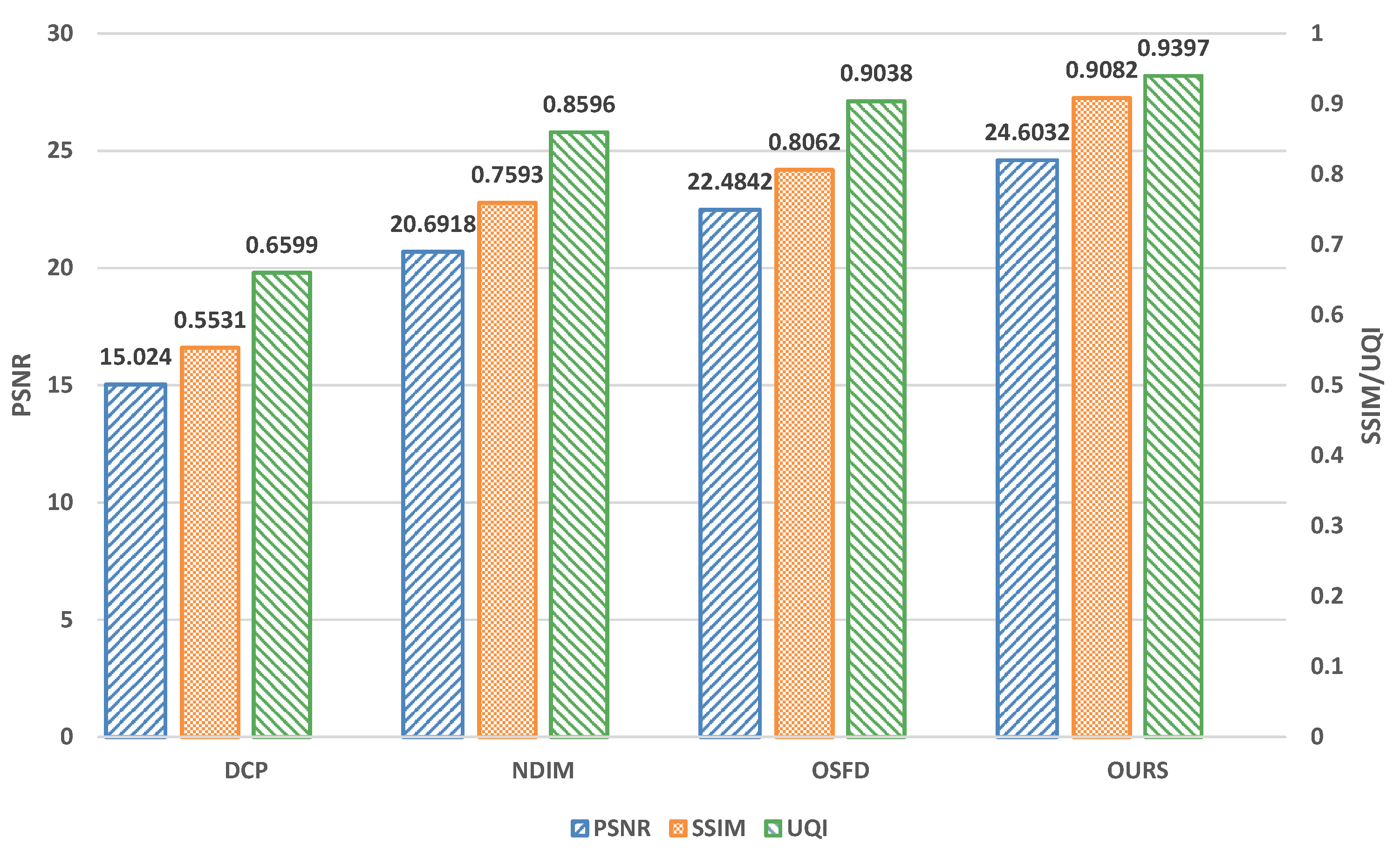
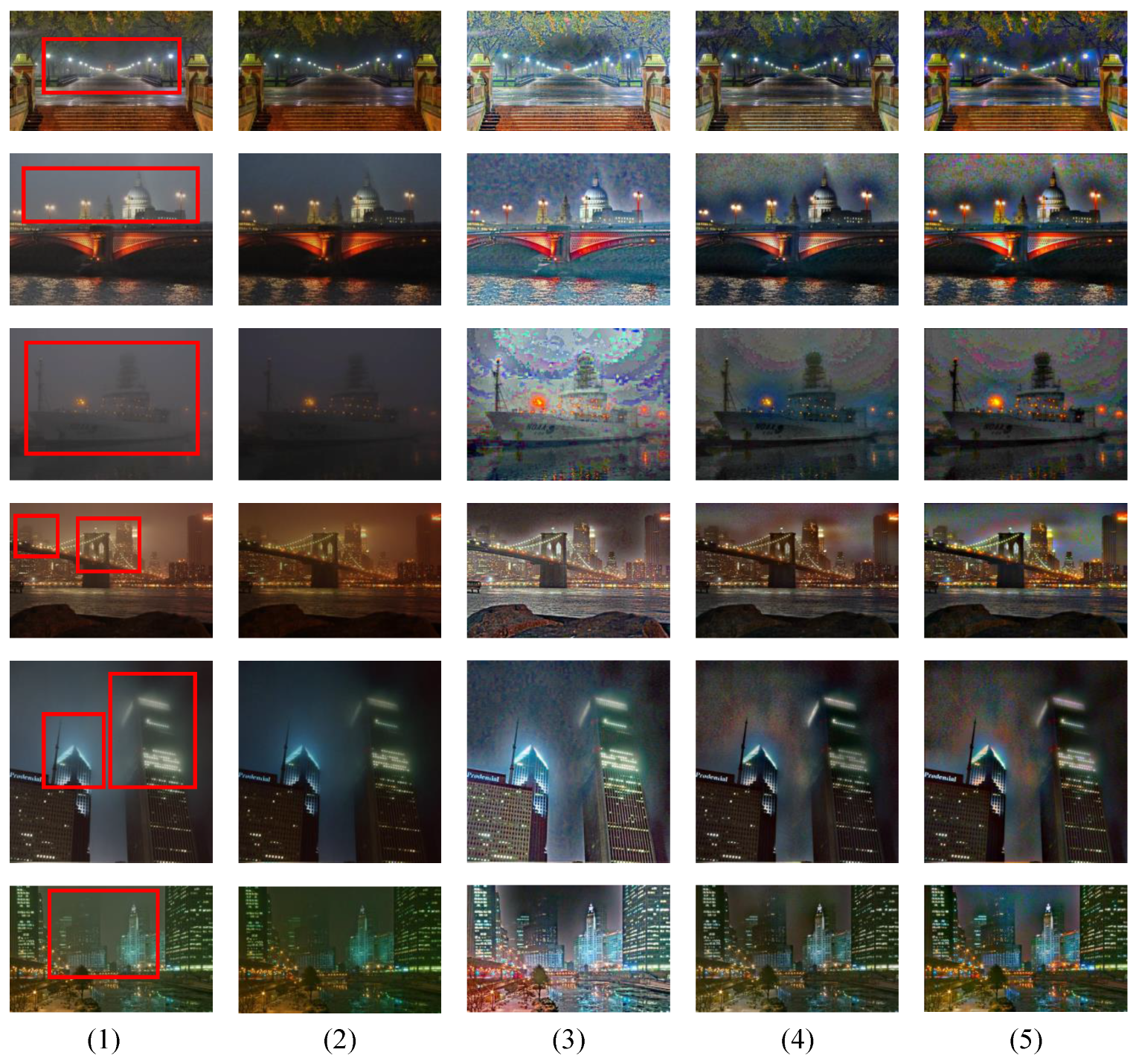
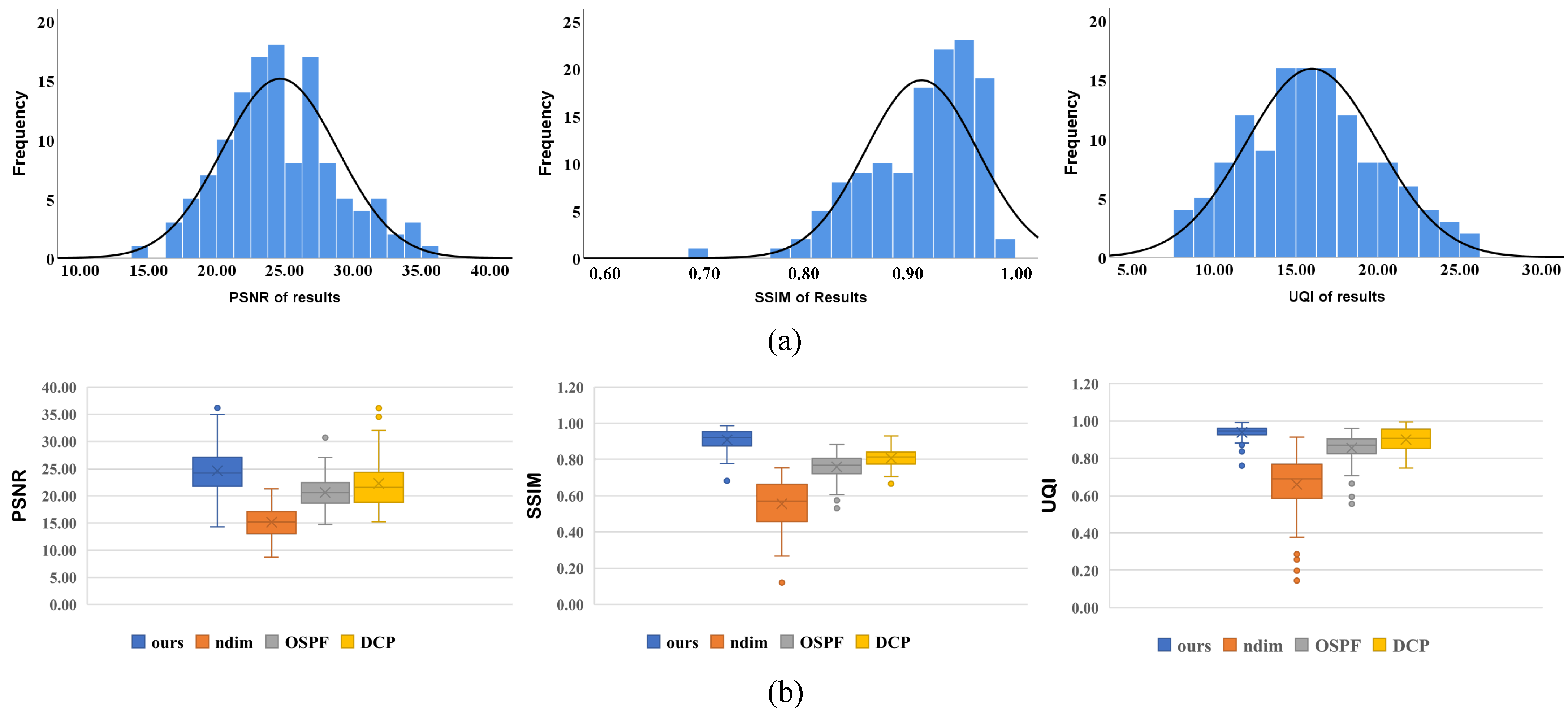
In this paper, a nighttime dehazing algorithm based on the light source influence matrix is proposed for the foggy environment at night. Different from the DCP estimation method of constant atmospheric light values, our light source influence matrix is more suitable for night scenes. Furthermore, the processed image by our method does not occur overexposed near the light source. To enhance the detail of image, an edge filter is introduced to fuse the transmittance of the near and far light source areas, and the correction with MRP makes the image more colorful. In addition, we introduce bias coefficients to make the algorithm effective in dense fog situations. Therefore, our method is better adapted to night scenes. The performance of the algorithm is quantitatively analyzed from three aspects: PSNR, SSIM, and UQI. The experimental results show that the proposed algorithm is effective in removing fog at night. In terms of PSNR, SSIM, and UQI, this method improves 34%, 22%, and 21% over the existed night-time defogging method OSPF. However, the time complexity of the algorithm increases as the size of the image increases. Refining the dark part and maintaining the time complexity is the main direction of future research. With the development of artificial intelligence, 5G communication, and other technologies, the next step will be to improve the dehazing algorithm to achieve video stream dehazing, or integrate the dehazing algorithm improvement into the target detection field.

References

1. Chen, C.; Li, S.; Qin, H.; Pan, Z.; Yang, G. Bilevel Feature Learning for Video Saliency Detection. IEEE Trans. Multim. 2018, 20, 3324–3336. [Google Scholar] [CrossRef]
2. Liu, W.; Ren, G.; Yu, R.; Guo, S.; Zhu, J.; Zhang, L. Image-Adaptive YOLO for Object Detection in Adverse Weather Conditions. In Proceedings of the Thirty-Sixth AAAI Conference on Artificial Intelligence, AAAI 2022, Thirty-Fourth Conference on Innovative Applications of Artificial Intelligence, IAAI 2022, The Twelveth Symposium on Educational Advances in Artificial Intelligence, EAAI 2022, Virtual, 22 February–1 March 2022; pp. 1792–1800. [Google Scholar]
3. Chen, J.; Yang, G.; Ding, X.; Guo, Z.; Wang, S. Robust detection of dehazed images via dual-stream CNNs with adaptive feature fusion. Comput. Vis. Image Underst. 2022, 217, 103357. [Google Scholar] [CrossRef]
4. Tsai, C.Y.; Chen, C.L. Attention-Gate-Based Model with Inception-like Block for Single-Image Dehazing. Appl. Sci. 2022, 12, 6725. [Google Scholar] [CrossRef]
5. Dong, H.; Pan, J.; Xiang, L.; Hu, Z.; Zhang, X.; Wang, F.; Yang, M.H. Multi-scale boosted dehazing network with dense feature fusion. In Proceedings of the IEEE/CVF Conference on Computer Vision and Pattern Recognition, Seattle, WA, USA, 13–19 June 2020; pp. 2157–2167. [Google Scholar]
6. Brown, M.; Süsstrunk, S. Multi-spectral SIFT for scene category recognition. In Proceedings of the CVPR 2011, Colorado Springs, CO, USA, 20–25 June 2011; pp. 177–184. [Google Scholar]
7. Sharma, T.; Shah, T.; Verma, N.K.; Vasikarla, S. A Review on Image Dehazing Algorithms for Vision based Applications in Outdoor Environment. In Proceedings of the 49th IEEE Applied Imagery Pattern Recognition Workshop, AIPR 2020, Washington, DC, USA, 13–15 October 2020; pp. 1–13. [Google Scholar] [CrossRef]
8. Schechner, Y.Y.; Narasimhan, S.G.; Nayar, S.K. Instant Dehazing of Images Using Polarization. In Proceedings of the 2001 IEEE Computer Society Conference on Computer Vision and Pattern Recognition (CVPR 2001), with CD-ROM, Kauai, HI, USA, 8–14 December 2001; pp. 325–332. [Google Scholar] [CrossRef] [Green Version]
9. Tan, R.T. Visibility in bad weather from a single image. In Proceedings of the 2008 IEEE Computer Society Conference on Computer Vision and Pattern Recognition (CVPR 2008), Anchorage, AK, USA, 24–26 June 2008. [Google Scholar] [CrossRef]
10. Ancuti, C.O.; Ancuti, C.; Bekaert, P. Effective single image dehazing by fusion. In Proceedings of the International Conference on Image Processing, ICIP 2010, Hong Kong, China, 26–29 September 2010; pp. 3541–3544. [Google Scholar] [CrossRef]
11. Banerjee, S.; Sinha Chaudhuri, S. Nighttime image-dehazing: A review and quantitative benchmarking. Arch. Comput. Methods Eng. 2021, 28, 2943–2975. [Google Scholar] [CrossRef]
12. Choi, L.K.; You, J.; Bovik, A.C. Referenceless Prediction of Perceptual Fog Density and Perceptual Image Defogging. IEEE Trans. Image Process. 2015, 24, 3888–3901. [Google Scholar] [CrossRef] [PubMed]
13. Howard, J.N. Scattering Phenomena: Optics of the Atmosphere. Scattering by Molecules and Particles. Earl J. McCartney. Wiley, New York, 1976. xviii, 408 pp., illus. Science 1977, 196, 1084–1085. [Google Scholar] [CrossRef]
14. He, K.; Sun, J.; Tang, X. Single Image Haze Removal Using Dark Channel Prior. IEEE Trans. Pattern Anal. Mach. Intell. 2011, 33, 2341–2353. [Google Scholar] [CrossRef]
15. Peng, Y.T.; Cao, K.; Cosman, P.C. Generalization of the dark channel prior for single image restoration. IEEE Trans. Image Process. 2018, 27, 2856–2868. [Google Scholar] [CrossRef] [PubMed]
16. Zhu, Q.; Mai, J.; Shao, L. A Fast Single Image Haze Removal Algorithm Using Color Attenuation Prior. IEEE Trans. Image Process. 2015, 24, 3522–3533. [Google Scholar] [CrossRef] [Green Version]
17. Zhu, Q.; Mai, J.; Shao, L. Single image dehazing using color attenuation prior. In Proceedings of the BMVC, Nottingham, UK, 1–5 September 2014. [Google Scholar]
18. Liu, Q.; Gao, X.; He, L.; Lu, W. Single image dehazing with depth-aware non-local total variation regularization. IEEE Trans. Image Process. 2018, 27, 5178–5191. [Google Scholar] [CrossRef]
19. Gui, J.; Cong, X.; Cao, Y.; Ren, W.; Zhang, J.; Zhang, J.; Tao, D. A Comprehensive Survey on Image Dehazing Based on Deep Learning. In Proceedings of the Thirtieth International Joint Conference on Artificial Intelligence, IJCAI 2021, Montreal, QC, Canada, 19–27 August 2021; Zhou, Z., Ed.; pp. 4426–4433. [Google Scholar] [CrossRef]
20. Kuanar, S.; Rao, K.R.; Mahapatra, D.; Bilas, M. Night Time Haze and Glow Removal using Deep Dilated Convolutional Network. arXiv 2019, arXiv:1902.00855v1. [Google Scholar]
21. Qu, Y.; Chen, Y.; Huang, J.; Xie, Y. Enhanced Pix2pix Dehazing Network. In Proceedings of the IEEE Conference on Computer Vision and Pattern Recognition, CVPR 2019, Long Beach, CA, USA, 16–20 June 2019; pp. 8160–8168. [Google Scholar] [CrossRef]
22. Zhu, H.; Peng, X.; Chandrasekhar, V.; Li, L.; Lim, J. DehazeGAN: When Image Dehazing Meets Differential Programming. In Proceedings of the Twenty-Seventh International Joint Conference on Artificial Intelligence, IJCAI 2018, Stockholm, Sweden, 13–19 July 2018; Lang, J., Ed.; pp. 1234–1240. [Google Scholar] [CrossRef] [Green Version]
23. Zhang, J.; Cao, Y.; Wang, Z. Nighttime haze removal based on a new imaging model. In Proceedings of the 2014 IEEE International Conference on Image Processing, ICIP 2014, Paris, France, 27–30 October 2014; pp. 4557–4561. [Google Scholar] [CrossRef]
24. Pei, S.; Lee, T. Nighttime haze removal using color transfer pre-processing and Dark Channel Prior. In Proceedings of the 19th IEEE International Conference on Image Processing, ICIP 2012, Lake Buena Vista, Orlando, FL, USA, 30 September–3 October 2012; pp. 957–960. [Google Scholar] [CrossRef]
25. Li, Y.; Tan, R.T.; Brown, M.S. Nighttime Haze Removal with Glow and Multiple Light Colors. In Proceedings of the 2015 IEEE International Conference on Computer Vision, ICCV 2015, Santiago, Chile, 7–13 December 2015; pp. 226–234. [Google Scholar] [CrossRef]
26. Land, E.H.; McCann, J.J. Lightness and retinex theory. Josa 1971, 61, 1–11. [Google Scholar] [CrossRef] [PubMed]
27. Yu, T.; Song, K.; Miao, P.; Yang, G.; Yang, H.; Chen, C. Nighttime Single Image Dehazing via Pixel-Wise Alpha Blending. IEEE Access 2019, 7, 114619–114630. [Google Scholar] [CrossRef]
28. Aiping, Y.; Nan, W. Nighttime Image Dehazing Algorithm by Structure-Texture Image Decomposition. Laser Optoelectron. Prog. 2018, 55, 061001. [Google Scholar] [CrossRef]
29. Harald, K. Theorie der Horizontalen Sichtweite: Kontrast und Sichtweite; Keim and Nemnich: Munich, Germany, 1924; Volume 12. [Google Scholar]
30. Narasimhan, S.G.; Nayar, S.K. Chromatic Framework for Vision in Bad Weather. In Proceedings of the 2000 Conference on Computer Vision and Pattern Recognition (CVPR 2000), Hilton Head, SC, USA, 13–15 June 2000; pp. 1598–1605. [Google Scholar] [CrossRef] [Green Version]
31. Yan, Y.; Zhang, S.; Ju, M.; Ren, W.; Wang, R.; Guo, Y. A point light source interference removal method for image dehazing. In Proceedings of the IEEE/CVF Conference on Computer Vision and Pattern Recognition Workshops, Seattle, WA, USA, 13–19 June 2020; pp. 874–875. [Google Scholar]
32. Zhang, J.; Cao, Y.; Fang, S.; Kang, Y.; Chen, C.W. Fast Haze Removal for Nighttime Image Using Maximum Reflectance Prior. In Proceedings of the 2017 IEEE Conference on Computer Vision and Pattern Recognition, CVPR 2017, Honolulu, HI, USA, 21–26 July 2017; pp. 7016–7024. [Google Scholar] [CrossRef]
33. Ancuti, C.; Ancuti, C.O.; Vleeschouwer, C.D.; Bovik, A.C. Night-time dehazing by fusion. In Proceedings of the 2016 IEEE International Conference on Image Processing, ICIP 2016, Phoenix, AZ, USA, 25–28 September 2016; pp. 2256–2260. [Google Scholar] [CrossRef]
34. Yang, A.; Zhao, M.; Wang, H.; Lu, L. Nighttime Image Dehazing Based on Low-Pass Filtering and Joint Optimization of Multi-Feature. Acta Opt. Sin. 2018, 38, 1010006. [Google Scholar] [CrossRef]
35. Zhang, J.; Cao, Y.; Zha, Z.; Tao, D. Nighttime Dehazing with a Synthetic Benchmark. In Proceedings of the MM’20: The 28th ACM International Conference on Multimedia, Seattle, WA, USA, 12–16 October 2020; Chen, C.W., Cucchiara, R., Hua, X., Qi, G., Ricci, E., Zhang, Z., Zimmermann, R., Eds.; ACM: New York, NY, USA, 2020; pp. 2355–2363. [Google Scholar] [CrossRef]
36. Hore, A.; Ziou, D. Image quality metrics: PSNR vs. SSIM. In Proceedings of the 2010 20th International Conference on Pattern Recognition, Istanbul, Turkey, 23–26 August 2010; pp. 2366–2369. [Google Scholar]
37. Sara, U.; Akter, M.; Uddin, M.S. Image quality assessment through FSIM, SSIM, MSE and PSNR—A comparative study. J. Comput. Commun. 2019, 7, 8–18. [Google Scholar] [CrossRef]
38. Ponomarenko, N.; Lukin, V.; Zelensky, A.; Egiazarian, K.; Carli, M.; Battisti, F. TID2008—A database for evaluation of full-reference visual quality assessment metrics. Adv. Mod. Radioelectron. 2009, 10, 30–45. [Google Scholar]
Figure 1. An overview of proposed nighttime dehazing method.
Applsci 12 10222 g001
Figure 2. The subjective experimental results. The defogging effect can be clearly seen at the red box. (1) Nighttime hazy image. (2) DCP [14]. (3) NDIM [25]. (4) OSFD [35]. (5) OURS.
Applsci 12 10222 g002
Figure 3. Image detail comparison. The defogging effect can be clearly seen at the red box.
Applsci 12 10222 g003
Figure 4. Performance comparison of different methods.
Applsci 12 10222 g004
Figure 5. The objective experimental results. The defogging effect can be clearly seen at the red box (1) Nighttime hazy image. (2) DCP [14]. (3) NDIM [25]. (4) OSFD [35]. (5) OURS.
Applsci 12 10222 g005
Figure 6. Statistics of the results. (a) Histogram of results; (b) Box diagram of different methods.
Applsci 12 10222 g006
Figure 7. Results of dehazing at different concentrations. ( α means the degree of fog concentration) (1) Origin image. (2) DCP [14]. (3) NDIM [25]. (4) OSFD [35]. (5) OURS.
Applsci 12 10222 g007