Einstein Aggregation Operators under Bipolar Neutrosophic Environment with Applications in Multi-Criteria Decision-Making

Abstract

In this article, we introduce bipolar neutrosophic (BN) aggregation operators (AOs) as a revolutionary notion in aggregation operators (AOs) by applying Einstein operations to bipolar neutrosophic aggregation operators (AOs), with its application related to a real-life problem. The neutrosophic set is able to drawout the incomplete, inconsistent and indeterminate information pretty efficiently. Initially, we present essential definitions along with operations correlated to the neutrosophic set (NS) and its generalization, the bipolar neutrosophic set (BNS). The Einstein aggregation operators are our primary targets, such asthe BN Einstein weighted average (BNEWA), BN Einstein ordered weighted average (BNEOWA), BN Einstein hybrid average (BNEHA), BN Einstein weighted geometric (BNEWG), BN Einstein ordered weighted geometric (BNEOWG) and BN Einstein hybrid geometric (BNEHG), as well as their required properties. The most important benefit of using the suggested approaches is that they provide decision-makers with complete sight of the issue. These techniques, when compared to other methods, provide complete, progressive and precise findings. Lastly, by means of diverse types of newly introduced aggregation operators and a numerical illustration by an example, we suggest an innovative method to be used for multi-criteria community decision-making (DM). This illustrates the utility and applicability of this new strategy when facing real-world problems.

1. Introduction

In the modern age of managerial decision-making (DM), knowledge frequently remains incomplete, undetermined and incompatible. L. A. Zadeh was the first to propose the fuzzy set theory [1], which deals with uncertainty and has applications in a wide range of modern fields of present and future society. Yet, fuzzy set has a problem in that it can simply convey the value of membership butnot non-membership. To address this, Atanassov [2] developed the intuitionistic fuzzy set (IFS), as well as associated theory, in order to summarizethe concept of fuzzy set.A pair of membership values is used to represent each IFS element, truth-membership $\Im \left(\chi \right)$ and a non-membership value (falsity-membership) $ƒ\left(\chi \right)$, as well as satisfy the condition $\Im \left(\chi \right),ƒ\left(\chi \right)\in \left[0,1\right]$ with $0\le \Im \left(\chi \right)+ƒ\left(\chi \right)\le 1$. IFS can only handle incomplete data, meaningindeterminate data are not an option.

Florentin Smarandache [3] developed the novel concept of NS, which adds an indeterminacy membership value ${\rm I}\left(\chi \right)$ to IFS. NS has a strong ability to deal with knowledge that is imperfect, uncertain and contradicting.

When $\Im \left(\chi \right)+{\rm I}\left(\chi \right)+ƒ\left(\chi \right)<1$, the information acquired is indeterminate.

When $\Im \left(\chi \right)+{\rm I}\left(\chi \right)+ƒ\left(\chi \right)>1$, this represents inconsistency in an NS.

Wang and others devised the single-valued neutrosophic set (SVNS) to deal with real-world situations [4], with the conditions $\Im \left(\chi \right),{\rm I}\left(\chi \right),ƒ\left(\chi \right)\in \left[0,1\right]$ and $0\le \Im \left(\chi \right)+{\rm I}\left(\chi \right)+ƒ\left(\chi \right)\le 3$. Ye [5] proposed a method for comparing SVNS, and defined the correlation coefficient.Wang et al. formulated an interval-valued neutrosophic set [6] and broadened the values of truth, indeterminacy and false memberships, which are all between 0 and 1.

For researchers, aggregation operators (AOs) are extremely important.Since its introduction, several scientists [7,8,9,10,11,12,13,14] have contributed significantly to the theory development of IFS. Xu et al. [15] introduced the concept of distinct IF aggregation operators based on IFS (AOs).Wang et al. and Zhao et al. [16,17] created Einstein aggregation operators (AOs). The Einstein t-norm typically gives the same smooth approximations as the product and sum of algebra.

The algebraic t-norm (product $\otimes$) and t-conorm (sum $\oplus$), respectively, are as below:

$$\begin{array}{l}T\left(a,b\right)=a\otimes b=ab\\ T^{\ast }\left(a,b\right)=a\oplus b=a+b-ab\end{array}$$

The Einstein operations t-norm (product $\otimes$) and t-conorm (sum $\oplus$), respectively, are as below:

$$\begin{array}{l}T\left(a,b\right)=a\otimes b=\frac{ab}{1+\left(1-a\right)\left(1-b\right)}\\ T^{\ast }\left(a,b\right)=a\oplus b=\frac{a+b}{1+ab}\end{array}$$

The bipolar fuzzy set (BFS) [18,19,20] has emerged as a new technique to deal with vagueness in DM situations.The bipolar fuzzy set’s membership degree varies between −1 and 1. Positive as well as negative membership degrees are available in BFS. BFSs are incredibly beneficial for several fields of study, as well as DM [21,22]. Gul [23] defined bipolar averaging and geometric aggregations operators (AOs). The bipolar neutrosophic set was created by Irfan and others [24,25] by using fundamental operations and a comparison mechanism [26,27]. Jamil and others created aggregation operators (AOs) based on BN values and applied them to DM problems. Heronian mean aggregation operators were developed by Fan and others [28]. Abdullah et al. introduced the idea of a bipolar soft set and its application to decision-making [29]. Jafar and other developed a bipolar neutrosophic soft set and applied itto decision-making [30]. Ali et al. introduced complex fuzzy set and its properties [31]. Broumi et al. introduced bipolar complex fuzzy set and its aggregation operators [32]. Jamil and others applieda multi-criteria decision-making approach to the bipolar neutrosophic set [33].

Regardless of the available information, there isa lot of literature related to the subject. The following features of the bipolar neutrosophic set inspired the present research team to perform a systematic and in-depth inquiry into decision analysis. Our findings are given below:

SVNSs deal with ambiguous details easily. This set combines the generalization of prior sets such as the classical set, the FS set and the IFS set.BFSs are highly effective for dealing withunpredictable, unexpected real-world circumstances because these can handle both positive as well as negative membership values.

The current study’s main and most important goals were as follows:

• To suggest different bipolar neutrosophic Einstein AOs as well as desired properties to study;
• Based on BNN, establish a multi-criteria DM approach in the direction of real life problem-solving;
• Give a numerical description of amulti-criteria DM example.

The remainder of the paper is organized at follows. The second segment presents a basic definition as well as its associated properties.The BNEWA and BNEWG aggregation operators are introduced in the Section 3.These innovative AOs are applied to multi-criteria decision-making in Section 4, and a numerical example is also presented.Finally, we offer comparative research, as well as some concluding thoughts, in Section 5.

2. Preliminaries

In this section, we provide fundamental definitions related to neutrosophic set theory. We define different fuzzy sets, BNS, scorefunctions, accuracyfunctions, and certainty functions, as well as the Einstein operations.

Definition 1 [3]. 

Consider R to represent a fixed set. Then, the neutrosophic set N is defined as:

$$N=\left\{ \left( \chi , \Im \left(\chi \right),{\rm I}\left(\chi \right),ƒ\left(\chi \right) \right) | \chi \in R\right\}$$

Now, the mapping for membership functions of truth, indeterminacy and falsity are$\Im :N\to Q$,${\rm I}:N\to Q$and$ƒ:N\to Q$, respectively; here,$Q=\left]0^{-},1^{+}\right[$and$0^{-}\le \Im \left(\chi \right)+{\rm I}\left(\chi \right)+ƒ\left(\chi \right)\le 3^{+}$.

Definition 2 [4]. 

Consider P to represent a fixed set; the single-valued neutrosophic set (SVNS) of A is stated as:

$$A_{NS}=\left\{\left(\chi ,\Im \left(\chi \right),{\rm I}\left(\chi \right),ƒ\left(\chi \right)\right)|\chi \in P\right\}$$

Now, here, the mapping for membership functions of truth, indeterminacy and falsity are$\Im :A_{NS}\to L$,${\rm I}:A_{NS}\to L$and$ƒ:A_{NS}\to L$, respectively; here,$L=\left[0,1\right]$and there is the condition$0\le \Im \left(\chi \right)+{\rm I}\left(\chi \right)+ƒ\left(\chi \right)\le 3$.

Some fundamental operations related to single-valued neutrosophic sets (SVNS) are listed below:

$$A_{NS}=\left\{\left(\chi ,{\Im }_{A_{NS}}\left(\chi \right),{{\rm I}}_{A_{NS}}\left(\chi \right),{ƒ}_{A_{NS}}\left(\chi \right)\right)|\chi \in P\right\},{ \mathrm{B}}_{NS}=\left\{\left(\chi ,{\Im }_{B_{NS}}\left(\chi \right),{{\rm I}}_{B_{NS}}\left(\chi \right),{ƒ}_{B_{NS}}\left(\chi \right)\right)|\chi \in P\right\},$$

The subset$A_{NS}\subseteq B_{NS}$is represented as

$${\Im }_{A_{NS}}\left(\chi \right)\le {\Im }_{B_{NS}}\left(\chi \right),{{\rm I}}_{A_{NS}}\left(\chi \right)\ge {{\rm I}}_{B_{NS}}\left(\chi \right),{ƒ}_{A_{NS}}\left(\chi \right)\ge {ƒ}_{B_{NS}}\left(\chi \right).$$

$A_{NS}=B_{NS}$is represented as

$${\Im }_{A_{NS}}\left(\chi \right)={\Im }_{B_{NS}}\left(\chi \right),{{\rm I}}_{A_{NS}}\left(\chi \right)={{\rm I}}_{B_{NS}}\left(\chi \right),{ƒ}_{A_{NS}}\left(\chi \right)={ƒ}_{B_{NS}}\left(\chi \right).$$

The complement$A_{NS}^{\prime }$is

$$A_{NS}^{\prime }=\left\{\left(\chi ,{ƒ}_{A_{NS}}\left(\chi \right),1-{{\rm I}}_{A_{NS}}\left(\chi \right),{\Im }_{A_{NS}}\left(\chi \right)\right)|\chi \in P\right\}$$

$A_{NS}\cap B_{NS}$is represented as

$$A_{NS}\cap B_{NS}=\left\{\left(\chi ,\min \left\{{\Im }_{A_{NS}}\left(\chi \right),{\Im }_{B_{NS}}\left(\chi \right)\right\},\max \left\{{{\rm I}}_{A_{NS}}\left(\chi \right),{{\rm I}}_{B_{NS}}\left(\chi \right)\right\},\max \left\{{ƒ}_{A_{NS}}\left(\chi \right),{ƒ}_{B_{NS}}\left(\chi \right)\right\}\right)|\chi \in P\right\}$$

The union is defined by

$$A_{NS}\cup B_{NS}=\left\{\left(\chi ,\max \left\{{\Im }_{A_{NS}}\left(\chi \right),{\Im }_{B_{NS}}\left(\chi \right)\right\},\min \left\{{{\rm I}}_{A_{NS}}\left(\chi \right),{{\rm I}}_{B_{NS}}\left(\chi \right)\right\},\min \left\{{ƒ}_{A_{NS}}\left(\chi \right),{ƒ}_{B_{NS}}\left(\chi \right)\right\}\right)|\chi \in P\right\}$$

Definition 3 [5]. 

Consider two single-valued neutrosophic numbers (SVNNs)$u_1=\left({\Im }_1,{{\rm I}}_1,{ƒ}_1\right)$and$u_2=\left({\Im }_2,{{\rm I}}_2,{ƒ}_2\right)$. The following are the distinct basic operations for SVNNs:

$$\begin{array}{c}{u}_1+u_2=\left({\Im }_1+{\Im }_2-{\Im }_1{\Im }_2,{{\rm I}}_1{{\rm I}}_2,{ƒ}_1{ƒ}_2\right); \\ u_1\cdot u_2=\left({\Im }_1+{\Im }_2,{{\rm I}}_1+{{\rm I}}_2-{{\rm I}}_1{{\rm I}}_2,{ƒ}_1+{ƒ}_2-{ƒ}_1{ƒ}_2\right); \\ \lambda \left(u_1\right)=\left(1-{\left(1-{\Im }_1\right)}^{\lambda },{\left({{\rm I}}_1\right)}^{\lambda },{\left({ƒ}_1\right)}^{\lambda }\right); \\ {\left(u_1\right)}^{\lambda }=\left({\left({\Im }_1\right)}^{\lambda },1-{\left(1-{{\rm I}}_1\right)}^{\lambda },1-{\left(1-{ƒ}_1\right)}^{\lambda }\right); \end{array}$$

where$\lambda >0$.

Definition 4 [5]. 

Let$u_1=\left({\Im }_1,{{\rm I}}_1,{ƒ}_1\right)$be a single-valued neutrosophic number (SVNN). Then, the score function$s\left(u_1\right)$is defined below:

$$s\left(u_1\right)=\frac{\left({\Im }_1+1-{{\rm I}}_1+1-{ƒ}_1\right)}{3};$$

Definition 5 [5]. 

The accuracy function for an SVNN$u_1=\left({\Im }_1,{{\rm I}}_1,{ƒ}_1\right)$is denoted by$\left(u_1\right)$, defined below:

$$\left(u_1\right)=\left({\Im }_1-{ƒ}_1\right);$$

Definition 6 [5]. 

The certainty function for an SVNN$u_1=\left({\Im }_1,{{\rm I}}_1,{ƒ}_1\right)$is denoted by$c\left(u_1\right)$, defined below:

$$c\left(u_1\right)={\Im }^{}{}_1$$

Definition 7 [5]. 

Consider two SVNNs$u_1=\left({\Im }_1,{{\rm I}}_1,{ƒ}_1\right)$and$u_2=\left({\Im }_2,{{\rm I}}_2,{ƒ}_2\right)$. The following is the relationship between them:

i. 

In condition$s(u_{{}_1})>s(u_{{}_2}),$then$u_1$is greater than$u_2$, denoted by$u_{{}_1}>u_2$;

ii. 

In condition$s(u_{{}_1})=s(u_2)$and a$\left(u_1\right)>$a$\left(u_2\right)$, then$u_1$is greater than$u_2$, denoted by$u_{{}_1}>u_2$;

iii. 

In condition$s(u_{{}_1})=s(u_2)$, a$\left(u_1\right)=$a$\left(u_2\right)$and$c(u_{{}_1})>c(u_2),$in that case,$u_1$is superior to$u_2$, denoted by$u_{{}_1}>u_2$;

iv. 

In condition$s(u_{{}_1})=s(u_2)$, a$\left(u_1\right)=$a$\left(u_2\right)$and$c(u_{{}_1})=c(u_2),$in that case,$u_1$is equal to$u_2$, denoted by$u_{{}_1}=u_2$;

Definition 8 [21]. 

Consider P as a universal set. Then, the bipolar fuzzy set (BFS) is stated below:

$$F=\left\{〈\chi ,{\Im }_F^{+}\left(\chi \right),{ƒ}_F^{-}\left(\chi \right)〉|\chi \in P^{}\right\}$$

where${\Im }_{{}_{{}^F}}^{+}\left(\chi \right):F\to L^{+}$represents a positive membership function and the negative membership function is${ƒ}_{{}_F}^{-}\left(\chi \right):F\to K^{-},$where$L^{+}=\left[0{,}^{}1\right]$and$K^{-}=\left[-1{,}^{}0\right].$

Definition 9 [25]. 

Suppose A is a bipolar neutrosophic set contained by universal set P, stated as:

$$A^{}=\left\{{}_{}{\left(\chi {,}^{}{\Im }^{+}\left(\chi \right){,}_{}{{\rm I}}^{+}\left(\chi \right){,}^{}{ƒ}^{+}\left(\chi \right){,}_{}{\Im }^{-}\left(\chi \right){,}^{}{{\rm I}}^{-}\left(\chi \right){,}_{}{ƒ}^{-}\left(\chi \right)\right)}_{}{|}^{}\chi \in P\right\}$$

Let${\Im }^{+}\left(\chi \right),{{\rm I}}^{+}\left(\chi \right),{ƒ}^{+}\left(\chi \right)=B{N}^{+}$as well as${\Im }^{-}\left(\chi \right),{{\rm I}}^{-}\left(\chi \right),{ƒ}^{-}\left(\chi \right)=B{N}^{-}.$

Here,${\Im }^{+}\left(\chi \right),{{\rm I}}^{+}\left(\chi \right),{ƒ}^{+}\left(\chi \right)$are positive membership functions representingtrue, indeterminate and false for$\chi \in P$, and${\Im }^{-}\left(\chi \right),{{\rm I}}^{-}\left(\chi \right),{ƒ}^{-}\left(\chi \right)$represent true, indeterminate and false for negative membership functions. Now, when mapping$B{N}^{+}:A\to L^{+}$and$B{N}^{-}:A\to L^{-},$here,$L^{+}=\left[0{,}^{}1\right]$and$L^{-}=\left[-1{,}^{}0\right].$This applies with the condition$0\le {\Im }^{+}\left(\chi \right)+{{\rm I}}^{+}\left(\chi \right)+{ƒ}^{+}\left(\chi \right)+{\Im }^{-}\left(\chi \right)+{{\rm I}}^{-}\left(\chi \right)+{ƒ}^{-}\left(\chi \right)\le 6$.

Example 1. 

Let$P=\left\{{\chi }_1,{\chi }_2,{\chi }_3\right\}$, then

$$A=\left\{\begin{array}{l}\left({\chi }_1,0.1,0.5,0.3,-0.4,-0.5,-0.6\right),\\ \left({\chi }_2,0.2,0.7,0.4,-0.3,-0.6,-0.2\right),\\ \left({\chi }_3,0.4,0.6,0.7,-0.2,-0.3,-0.1\right)\end{array}\right\}$$

is a subset of universal set P that is BNS.

Some fundamental operations [12] used for BNSs are stated below:

Let $A_1=\left\{\left(\chi ,{\Im }_1^{+}\left(\chi \right),{{\rm I}}_1^{+}\left(\chi \right),{ƒ}_1^{+}\left(\chi \right),{\Im }_1^{-}\left(\chi \right),{{\rm I}}_1^{-}\left(\chi \right),{ƒ}_1^{-}\left(\chi \right)\right)|\chi \in P\right\}$ and $A_2=\left\{\left(\chi ,{\Im }_2^{+}\left(\chi \right),{{\rm I}}_2^{+}\left(\chi \right),{ƒ}_2^{+}\left(\chi \right),{\Im }_2^{-}\left(\chi \right),{{\rm I}}_2^{-}\left(\chi \right),{ƒ}_2^{-}\left(\chi \right)\right)|\chi \in P\right\}$ be two BNSs.

i.

Then,$A_1\subseteq A_2$ if and only if

$${\Im }_1^{+}\left(\chi \right)\le {\Im }_2^{+}\left(\chi \right),{{\rm I}}_1^{+}\left(\chi \right)\le {{\rm I}}_2^{+}\left(\chi \right),{ƒ}_1^{+}\left(\chi \right)\ge {ƒ}_2^{+}\left(\chi \right),$$

and

$${\Im }_1^{-}\left(\chi \right)\ge {\Im }_2^{-}\left(\chi \right),{{\rm I}}_1^{-}\left(\chi \right)\ge {{\rm I}}_2^{-}\left(\chi \right),{ƒ}_1^{-}\left(\chi \right)\le {ƒ}_2^{-}\left(\chi \right)$$

ii. 

$A_1=A_2$ if and only if

$${\Im }_1^{+}\left(\chi \right)={\Im }_2^{+}\left(\chi \right),{{\rm I}}_1^{+}\left(\chi \right)={{\rm I}}_2^{+}\left(\chi \right),{ƒ}_1^{+}\left(\chi \right)={ƒ}_2^{+}\left(\chi \right),$$

and

$${\Im }_1^{-}\left(\chi \right)={\Im }_2^{-}\left(\chi \right),{{\rm I}}_1^{-}\left(\chi \right)={{\rm I}}_2^{-}\left(\chi \right),{ƒ}_1^{-}\left(\chi \right)={ƒ}_2^{-}\left(\chi \right)$$

iii. 

The union is defined as below:

$$\left(A_1\cup A_2\right)=\left\{\left(\max \left({\Im }_1^{+}\left(\chi \right),{\Im }_2^{+}\left(\chi \right)\right),\frac{{{\rm I}}_1^{+}\left(\chi \right)+{{\rm I}}_2^{+}\left(\chi \right)}{2},\min \left({ƒ}_1^{+}\left(\chi \right),{ƒ}_2^{+}\left(\chi \right)\right),\min \left({\Im }_1^{-}\left(\chi \right),{\Im }_2^{-}\left(\chi \right)\right),\frac{{{\rm I}}_1^{-}\left(\chi \right)+{{\rm I}}_2^{-}\left(\chi \right)}{2},\max \left({ƒ}_1^{-}\left(\chi \right),{ƒ}_2^{-}\left(\chi \right)\right)\right)\right\},$$

iv. 

The intersection is defined as:

$$\left(A_1\cap A_2\right)=\left\{\left(\min \left({\Im }_1^{+}\left(\chi \right),{\Im }_2^{+}\left(\chi \right)\right),\frac{{{\rm I}}_1^{+}\left(\chi \right)+{{\rm I}}_2^{+}\left(\chi \right)}{2},\max \left({ƒ}_1^{+}\left(\chi \right),{ƒ}_2^{+}\left(\chi \right)\right),\max \left({\Im }_1^{-}\left(\chi \right),{\Im }_2^{-}\left(\chi \right)\right),\frac{{{\rm I}}_1^{-}\left(\chi \right)+{{\rm I}}_2^{-}\left(\chi \right)}{2},\min \left({ƒ}_1^{-}\left(\chi \right),{ƒ}_2^{-}\left(\chi \right)\right)\right)\right\},$$

v. 

Let $A=\left\{\left(\chi ,{\Im }^{+}\left(\chi \right),{{\rm I}}^{+}\left(\chi \right),{ƒ}^{+}\left(\chi \right),{\Im }^{-}\left(\chi \right),{{\rm I}}^{-}\left(\chi \right),{ƒ}^{-}\left(\chi \right)\right)|\chi \in P\right\}$ be BNSs.

Then, the complement $A^{\prime }$ is defined as:

$${\Im }_{A^{\prime }}^{+}\left(\chi \right)=\left\{1^{+}\right\}-{\Im }_A^{+}\left(\chi \right),{{\rm I}}_{A^{\prime }}^{+}\left(\chi \right)=\left\{1^{+}\right\}-{{\rm I}}_A^{+}\left(\chi \right),{ƒ}_{A^{\prime }}^{+}\left(\chi \right)=\left\{1^{+}\right\}-{ƒ}_A^{+}\left(\chi \right),$$

and

$${\Im }_{A^{\prime }}^{-}\left(\chi \right)=\left\{1^{-}\right\}-{\Im }_A^{-}\left(\chi \right),{{\rm I}}_{A^{\prime }}^{-}\left(\chi \right)=\left\{1^{-}\right\}-{{\rm I}}_A^{-}\left(\chi \right),{ƒ}_{A^{\prime }}^{-}\left(\chi \right)=\left\{1^{-}\right\}-{ƒ}_A^{-}\left(\chi \right),$$

Definition 10 [25]. 

Consider two bipolar neutrosophic numbers (BNNs)$u_1=\left({\Im }_1^{+},{{\rm I}}_1^{+},{ƒ}_1^{+},{\Im }_1^{-},{{\rm I}}_1^{-},{ƒ}_1^{-}\right)$and$u_2=\left({\Im }_2^{+},{{\rm I}}_2^{+},{ƒ}_2^{+},{\Im }_2^{-},{{\rm I}}_2^{-},{ƒ}_2^{-}\right)$. The following are the basic operations between two BNNs:

$$\begin{gathered} \mathrm{i}.u_1+u_2=\left({\Im }_1^{+}+{\Im }_2^{+}-{\Im }_1^{+}{\Im }_2^{+},{{\rm I}}_1^{+}{{\rm I}}_2^{+},{ƒ}_1^{+}{ƒ}_2^{+},-{\Im }_1^{-}{\Im }_2^{-},-\left(-{{\rm I}}_1^{-}-{{\rm I}}_2^{-}-{{\rm I}}_1^{-}{{\rm I}}_2^{-}\right),-\left(-{ƒ}_1^{-}-{ƒ}_2^{-}-{ƒ}_1^{-}{ƒ}_2^{-}\right)\right); \\ \mathrm{ii}.u_1\cdot u_2=\left({\Im }_1^{+}{\Im }_2^{+},{{\rm I}}_1^{+}+{{\rm I}}_2^{+}-{{\rm I}}_1^{+}{{\rm I}}_2^{+},{ƒ}_1^{+}+{ƒ}_2^{+}-{ƒ}_1^{+}{ƒ}_2^{+},-\left(-{\Im }_1^{-}-{\Im }_2^{-}-{\Im }_1^{-}{\Im }_2^{-}\right),-{{\rm I}}_1^{-}{{\rm I}}_2^{-},-{ƒ}_1^{-}{ƒ}_2^{-}\right); \\ \mathrm{iii}.\lambda \left(u_1\right)=\left(1-{\left(1-{\Im }_1^{+}\right)}^{\lambda },{\left({{\rm I}}_1^{+}\right)}^{\lambda },{\left({ƒ}_1^{+}\right)}^{\lambda },-{\left(-{\Im }_1^{-}\right)}^{\lambda },-{\left(-{{\rm I}}_1^{-}\right)}^{\lambda },-\left(1-{\left(1-\left(-{ƒ}_1^{-}\right)\right)}^{\lambda }\right)\right); \\ \mathrm{iv}.{\left(u_1\right)}^{\lambda }=\left({\left({\Im }_1^{+}\right)}^{\lambda },1-{\left(1-{{\rm I}}_1^{+}\right)}^{\lambda },1-{\left(1-{ƒ}_1^{+}\right)}^{\lambda },-\left(1-{\left(1-\left(-{\Im }_1^{-}\right)\right)}^{\lambda }\right),-{\left(-{{\rm I}}_1^{-}\right)}^{\lambda },-{\left(-{ƒ}_1^{-}\right)}^{\lambda }\right); \end{gathered}$$

where$\lambda >0$.

Definition 11 [25]. 

The score function for a bipolar neutrosophic number$u=\left({\Im }^{+},{{\rm I}}^{+},{ƒ}^{+},{\Im }^{-},{{\rm I}}^{-},{ƒ}^{-}\right)$denoted by$S\left(u\right)$is:

$$S\left(u\right)=\frac{1}{6}\left({\Im }^{+}+1-{{\rm I}}^{+}+1-{ƒ}^{+}+1+{\Im }^{-}-{{\rm I}}^{-}-{ƒ}^{-}\right)$$

Definition 12 [25]. 

The accuracy function defined for a BNN$u=\left({\Im }^{+}{}^{},{{\rm I}}^{+}{}_{},{ƒ}^{+}{}^{},{\Im }^{-}{,}_{}{{\rm I}}^{-},{ƒ}^{-}\right)$is$a\left({}_{}u\right)$, as below:

$$a\left({}_{}u\right)={\Im }^{+}-{ƒ}^{+}+{\Im }^{-}-{ƒ}^{-}$$

Definition 13 [25]. 

Consider$u=\left({\Im }^{+},{{\rm I}}^{+},{ƒ}^{+},{\Im }^{-},{{\rm I}}^{-},{ƒ}^{-}\right)$to represent the neutrosophic number. Then, thecertainty function is:

$$c_{}{\left(u\right)}^{}={ }_{}{\Im }_{}{}^{+}-{ƒ}^{}{}^{-}$$

Definition 14 [25]. 

Consider$u_1=\left({\Im }_1^{+},{{\rm I}}_1^{+},{ƒ}_1^{+},{\Im }_1^{-},{{\rm I}}_1^{-},{ƒ}_1^{-}\right)$and$u_2=\left({\Im }_2^{+},{{\rm I}}_2^{+},{ƒ}_2^{+},{\Im }_2^{-},{{\rm I}}_2^{-},{ƒ}_2^{-}\right)$to represent two BNNs. Then, acomparison method among BNNs is:

i. 

In condition$S(u_1)\succ S(u_2)$then$u_1$is greater than$u_2$, denoted by$u_1\succ u_2$

ii. 

In condition$S(u_1)=S(u_2)$and$a(u_1)\succ a(u_2)$then$u_1$is greater than$u_2$, denoted by$u_1\succ u_2;$

iii. 

In condition$S(u_1)=S(u_2),$$a(u_1)=a(u_2)$and$c(u_1)\succ c(u_2)$in that case,$u_1$is superior to$u_2$, denote by$u_1\succ u_2;$

iv. 

In condition$S(u_1)=S(u_2),$$a(u_1)=a(u_2)$and$c(u_1)=c(u_2)$in that case,$u_1$is equal to$u_2$, denoted by$u_1=u_2.$

Definition 15.

Consider$u=\left({\Im }^{+},{{\rm I}}^{+},{ƒ}^{+},{\Im }^{-},{{\rm I}}^{-},{ƒ}^{-}\right)$,$u_1=\left({\Im }_1^{+},{{\rm I}}_1^{+},{ƒ}_1^{+},{\Im }_1^{-},{{\rm I}}_1^{-},{ƒ}_1^{-}\right)$and$u_2=\left({\Im }_2^{+},{{\rm I}}_2^{+},{ƒ}_2^{+},{\Im }_2^{-},{{\rm I}}_2^{-},{ƒ}_2^{-}\right)$to be BNNs, and$\lambda \succ 0$any real value. Then, the fundamental Einstein operations of BNNs are:

$$\begin{gathered} u_1\oplus u_2=\left(\frac{{\Im }_1^{+}+{\Im }_2^{+}}{1+{\Im }_1^{+}{\Im }_2^{+}},\frac{{{\rm I}}_1^{+}{{\rm I}}_2^{+}}{1+\left(1-{{\rm I}}_1^{+}\right)\left(1-{{\rm I}}_2^{+}\right)},\frac{{ƒ}_1^{+}{ƒ}_2^{+}}{1+\left(1-{ƒ}_1^{+}\right)\left(1-{ƒ}_2^{+}\right)},\frac{-{\Im }_1^{-}{\Im }_2^{-}}{1+\left(1+{\Im }_1^{-}\right)\left(1+{\Im }_2^{-}\right)},\frac{-\left(-{{\rm I}}_1^{-}-{{\rm I}}_2^{-}\right)}{1+{{\rm I}}_1^{-}{{\rm I}}_2^{-}},\frac{-\left(-{ƒ}_1^{-}-{ƒ}_2^{-}\right)}{1+{ƒ}_1^{-}{ƒ}_2^{-}}\right) \\ {u}_1\otimes u_2=\left(\frac{{\Im }_1^{+}{\Im }_2^{+}}{1+\left(1-{\Im }_1^{+}\right)\left(1-{\Im }_2^{+}\right)},\frac{{{\rm I}}_1^{+}+{{\rm I}}_2^{+}}{1+{{\rm I}}_1^{+}{{\rm I}}_2^{+}},\frac{{ƒ}_1^{+}+{ƒ}_2^{+}}{1+{ƒ}_1^{+}{ƒ}_2^{+}},\frac{-\left(-{\Im }_1^{-}-{\Im }_2^{-}\right)}{1+{\Im }_1^{-}{\Im }_2^{-}},\frac{-{{\rm I}}_1^{-}{{\rm I}}_2^{-}}{1+\left(1+{{\rm I}}_1^{-}\right)\left(1+{{\rm I}}_2^{-}\right)},\frac{-{ƒ}_1^{-}{ƒ}_2^{-}}{1+\left(1+{ƒ}_1^{-}\right)\left(1+{ƒ}_2^{-}\right)}\right) \\ \lambda \left(u\right)=\left(\frac{{\left(1+{\Im }^{+}\right)}^{\lambda }-{\left(1-{\Im }^{+}\right)}^{\lambda }}{{\left(1+{\Im }^{+}\right)}^{\lambda }+{\left(1-{\Im }^{+}\right)}^{\lambda }},\frac{2{\left({{\rm I}}^{+}\right)}^{\lambda }}{{\left(2-{{\rm I}}^{+}\right)}^{\lambda }+{\left({{\rm I}}^{+}\right)}^{\lambda }},\frac{2{\left({ƒ}^{+}\right)}^{\lambda }}{{\left(2-{ƒ}^{+}\right)}^{\lambda }+{\left({ƒ}^{+}\right)}^{\lambda }},\frac{-2{\left|{\Im }^{-}\right|}^{\lambda }}{{\left(2+{\Im }^{-}\right)}^{\lambda }+{\left|{\Im }^{-}\right|}^{\lambda }},\frac{-2{\left|{{\rm I}}^{-}\right|}^{\lambda }}{{\left(2+{{\rm I}}^{-}\right)}^{\lambda }+{\left|{{\rm I}}^{-}\right|}^{\lambda }},\frac{-\left({\left(1+\left|{ƒ}^{-}\right|\right)}^{\lambda }-{\left(1+{ƒ}^{-}\right)}^{\lambda }\right)}{{\left(1+\left|{ƒ}^{-}\right|\right)}^{\lambda }+{\left(1+{ƒ}^{-}\right)}^{\lambda }}\right) \\ {\left(u\right)}^{\lambda }=\left(\frac{2{\left({\Im }^{+}\right)}^{\lambda }}{{\left(2-{\Im }^{+}\right)}^{\lambda }+{\left({\Im }^{+}\right)}^{\lambda }},\frac{{\left(1+{{\rm I}}^{+}\right)}^{\lambda }-{\left(1-{{\rm I}}^{+}\right)}^{\lambda }}{{\left(1+{{\rm I}}^{+}\right)}^{\lambda }+{\left(1-{{\rm I}}^{+}\right)}^{\lambda }},\frac{{\left(1+{ƒ}^{+}\right)}^{\lambda }-{\left(1-{ƒ}^{+}\right)}^{\lambda }}{{\left(1+{ƒ}^{+}\right)}^{\lambda }+{\left(1-{ƒ}^{+}\right)}^{\lambda }},\frac{-\left({\left(1+\left|{\Im }^{-}\right|\right)}^{\lambda }-{\left(1+{\Im }^{-}\right)}^{\lambda }\right)}{{\left(1+\left|{\Im }^{-}\right|\right)}^{\lambda }+{\left(1+{\Im }^{-}\right)}^{\lambda }},\frac{-2{\left|{{\rm I}}^{-}\right|}^{\lambda }}{{\left(2+{{\rm I}}^{-}\right)}^{\lambda }+{\left|{{\rm I}}^{-}\right|}^{\lambda }},\frac{-2{\left|{ƒ}^{-}\right|}^{\lambda }}{{\left(2+{ƒ}^{-}\right)}^{\lambda }+{\left|{ƒ}^{-}\right|}^{\lambda }}\right) \end{gathered}$$

3. Bipolar Neutrosophic Einstein Average AOs

Here, we suggest a number of fundamental properties for bipolar Einsteinaverage AOs in the current section of the article, such as BNEWA, BNEOWA and BNEHA.

3.1. Bipolar NeutrosophicEinstein Weighted-Average Aggregation Operators

Consider $u_l=\left({\Im }_l^{+},{{\rm I}}_l^{+},{ƒ}_l^{+},{\Im }_l^{-},{{\rm I}}_l^{-},{ƒ}_l^{-}\right)$ to represent a family of BNNs. Here, $l\in \left\{1,2,3,\dots ,n\right\}$

Definition 16.

The (BNEWA) aggregation operator is defined as follows:

$$BNEW{A}_{\nu }\left(u_1,u_2,\dots ,u_n\right)=\underset{l=1}{\overset{n}{\oplus }}\left({\nu }_l{u}_l\right)={\nu }_1{u}_1\oplus {\nu }_2{u}_2\oplus \dots \oplus {\nu }_n{u}_n$$

(1)

where$\nu ={\left({\nu }_1,{\nu }_2,\dots ,{\nu }_n\right)}^T$represents weighted vectors of$u_l$, that is,${\nu }_l>0$and${\displaystyle \sum _{l=1}^n}{\nu }_l=1$.

Theorem1. 

The (BNEWA) operator gives in return a (BNV) by

$$\begin{array}{l}BNEW{A}_{\nu }\left(u_1,u_2,\dots ,u_n\right)=\\ \left(\frac{{Ђ}_1-{Ђ}_2}{{Ђ}_1+{Ђ}_2},\frac{2{\zeta }_1}{{\zeta }_2+{\zeta }_1},\frac{2f_1}{f_2+f_1},\frac{-2{Ђ}_3}{{Ђ}_4+{Ђ}_3},-\frac{{\zeta }_3-{\zeta }_4}{{\zeta }_3+{\zeta }_4},-\frac{f_3-f_4}{f_3+f_4}\right)\end{array}$$

(2)

where

$$\begin{array}{l}{Ђ}_1={\displaystyle \prod _{{}_{l=1}}^n}{\left(1+{\Im }_l^{+}\right)}^{{\nu }_l},{Ђ}_2={\displaystyle \prod _{{}_{l=1}}^n}{\left(1-{\Im }_l^{+}\right)}^{{\nu }_l},{Ђ}_3={\displaystyle \prod _{l=1}^n}{\left|{\Im }_l^{-}\right|}^{{\nu }_l} , {Ђ}_4={\displaystyle \prod _{l{=}_{}1}^n}{\left(2+{\Im }_l^{-}\right)}^{{\nu }_l},\\ {\zeta }_1={\displaystyle \prod _{l=1}^n}{\left({{\rm I}}_l^{+}\right)}^{{\nu }_l},{\zeta }_2={\displaystyle \prod _{l=1}^n}{\left(2-{{\rm I}}_l^{+}\right)}^{{\nu }_l},{\zeta }_3={\displaystyle \prod _{l=1}^n}{\left(1+\left|{{\rm I}}_l^{-}\right|\right)}^{{\nu }_l},{\zeta }_4={\displaystyle \prod _{l=1}^n}{\left(1+{{\rm I}}_l^{-}\right)}^{{\nu }_l},\\ f_1={\displaystyle \prod _{l=1}^n}{\left({ƒ}_l^{+}\right)}^{{\nu }_l},f_2={\displaystyle \prod _{l=1}^n}{\left(2-{ƒ}_l^{+}\right)}^{{\nu }_l},f_3={\displaystyle \prod _{l=1}^n}{\left(1+\left|{ƒ}_l^{-}\right|\right)}^{{\nu }_l},f_4={\displaystyle \prod _{l=1}^n}{\left(1+{ƒ}_l^{-}\right)}^{{\nu }_l}. \\ \end{array}$$

where$\nu ={\left({\nu }_1,{\nu }_2,\dots ,{\nu }_n{}^{}\right)}_{}^{}{}^T$is the weighted vector of$u_l$,such that${\nu }_l>0$and${\displaystyle \sum _{l=1}^n}{\nu }_l=1$.

Proof. 

Now, by mathematical induction:

For $n=2$,

$${\nu }_1{u}_1=\left(\begin{array}{l}\frac{{\left(1+{\Im }_1^{+}\right)}^{{\nu }_1}-{\left(1-{\Im }_1^{+}\right)}^{{\nu }_1}}{{\left(1+{\Im }_1^{+}\right)}^{{\nu }_1}+{\left(1-{\Im }_1^{+}\right)}^{{\nu }_1}},\frac{2{\left({{\rm I}}_1^{+}\right)}^{{\nu }_1}}{{\left(2-{{\rm I}}_1^{+}\right)}^{{\nu }_1}+{\left({{\rm I}}_1^{+}\right)}^{{\nu }_1}},\frac{2{\left({ƒ}_1^{+}\right)}^{{\nu }_1}}{{\left(2-{ƒ}_1^{+}\right)}^{{\nu }_1}+{\left({ƒ}_1^{+}\right)}^{{\nu }_1}},\\ \frac{-2{\left|{\Im }_1^{-}\right|}^{{\nu }_1}}{{\left(2+{\Im }_1^{-}\right)}^{{\nu }_1}+{\left|{\Im }_1^{-}\right|}^{{\nu }_1}},\frac{-2{\left|{{\rm I}}_1^{-}\right|}^{{\nu }_1}}{{\left(2+{{\rm I}}_1^{-}\right)}^{{\nu }_1}+{\left|{{\rm I}}_1^{-}\right|}^{{\nu }_1}},\frac{-\left({\left(1+\left|{ƒ}_1^{-}\right|\right)}^{{\nu }_1}-{\left(1+{ƒ}_1^{-}\right)}^{{\nu }_1}\right)}{{\left(1+\left|{ƒ}_1^{-}\right|\right)}^{{\nu }_1}+{\left(1+{ƒ}_1^{-}\right)}^{{\nu }_1}}\end{array}\right)$$

and

$$\begin{array}{c}{\nu }_2{u}_2=\left(\begin{array}{l}\frac{{\left(1+{\Im }_2^{+}\right)}^{{\nu }_2}-{\left(1-{\Im }_2^{+}\right)}^{{\nu }_2}}{{\left(1+{\Im }_2^{+}\right)}^{{\nu }_2}+{\left(1-{\Im }_2^{+}\right)}^{{\nu }_2}},\frac{2{\left({{\rm I}}_2^{+}\right)}^{{\nu }_2}}{{\left(2-{{\rm I}}_2^{+}\right)}^{{\nu }_2}+{\left({{\rm I}}_2^{+}\right)}^{{\nu }_2}},\frac{2{\left({ƒ}_2^{+}\right)}^{{\nu }_2}}{{\left(2-{ƒ}_2^{+}\right)}^{{\nu }_2}+{\left({ƒ}_2^{+}\right)}^{{\nu }_2}},\\ \frac{-2{\left|{\Im }_2^{-}\right|}^{{\nu }_2}}{{\left(2+{\Im }_2^{-}\right)}^{{\nu }_2}+{\left|{\Im }_2^{-}\right|}^{{\nu }_2}},\frac{-2{\left|{{\rm I}}_2^{-}\right|}^{{\nu }_2}}{{\left(2+{{\rm I}}_2^{-}\right)}^{{\nu }_2}+{\left|{{\rm I}}_2^{-}\right|}^{{\nu }_2}},\frac{-\left({\left(1+\left|{ƒ}_2^{-}\right|\right)}^{{\nu }_2}-{\left(1+{ƒ}_2^{-}\right)}^{{\nu }_2}\right)}{{\left(1+\left|{ƒ}_2^{-}\right|\right)}^{{\nu }_2}+{\left(1+{ƒ}_2^{-}\right)}^{{\nu }_2}}\end{array}\right)\end{array}$$

and for

$${\nu }_1{u}_1=\left(\begin{array}{l}\frac{\left(1+{\Im }_1^{+}\right)-\left(1-{\Im }_1^{+}\right)}{\left(1+{\Im }_1^{+}\right)+\left(1-{\Im }_1^{+}\right)},\frac{2\left({{\rm I}}_1^{+}\right)}{\left(2-{{\rm I}}_1^{+}\right)+\left({{\rm I}}_1^{+}\right)},\frac{2\left({ƒ}_1^{+}\right)}{\left(2-{ƒ}_1^{+}\right)+\left({ƒ}_1^{+}\right)},\\ \frac{-2\left|{\Im }_1^{-}\right|}{\left(2+{\Im }_1^{-}\right)+\left|{\Im }_1^{-}\right|},-\frac{\left(1+\left|{{\rm I}}_1^{-}\right|\right)-\left(1+{{\rm I}}_1^{-}\right)}{\left(1+\left|{{\rm I}}_1^{-}\right|\right)+\left(1+{{\rm I}}_1^{-}\right)},-\frac{\left(1+\left|{ƒ}_1^{-}\right|\right)-\left(1+{ƒ}_1^{-}\right)}{\left(1+\left|{ƒ}_1^{-}\right|\right)+\left(1+{ƒ}_1^{-}\right)}\end{array}\right),$$

(3)

thus satisfying $n^{}{=}_{}1$.

We put $n^{}{=}_{}r$ into Equation (3)

$$\begin{array}{l}BNEW{A}_{\nu }\left(u_1,u_2,\dots ,u_r\right)=\\ \left(\begin{array}{l}\frac{{\displaystyle \prod _{{}_{l=1}}^r}{\left(1+{\Im }_l^{+}\right)}^{{\nu }_l}-{\displaystyle \prod _{l=1}^r}{\left(1-{\Im }_l^{+}\right)}^{{\nu }_l}}{{{\displaystyle \prod _{l=1}^r}}^{}{\left({}_{}1+{\Im }_l^{+}\right)}^{{\nu }_l}+{\displaystyle \prod _{l=1}^r}{\left(1-{\Im }_l^{+}\right)}^{{\nu }_l}},\frac{2{\displaystyle \prod _{l=1}^r}{\left({{\rm I}}_l^{+}\right)}^{{\nu }_l}}{{\displaystyle \prod _{l=1}^r}{\left(2-{{\rm I}}_l^{+}\right)}^{{\nu }_l}+{\displaystyle \prod _{l=1}^r}{\left({{\rm I}}_l^{+}\right)}^{{\nu }_l}},\frac{2{{\displaystyle \prod _{l=1}^r}}^{}{\left({}_{}{ƒ}_l^{+}\right)}^{{\nu }_l}}{{\displaystyle \prod _{l=1}^r}{\left(2-{ƒ}_l^{+}\right)}^{{\nu }_l}+{\displaystyle \prod _{l=1}^r}{\left({ƒ}_l^{+}\right)}^{{\nu }_l}},\\ \frac{-2{\displaystyle \prod _{l=1}^r}{\left|{\Im }_l^{-}\right|}^{{\nu }_l}}{{\displaystyle \prod _{l=1}^r}{\left(2+{\Im }_l^{-}\right)}^{{\nu }_l}+{\displaystyle \prod _{l=1}^r}{\left|{\Im }_l^{-}\right|}^{{\nu }_l}},\frac{-2{\displaystyle \prod _{l=1}^r}{\left|{{\rm I}}_l^{-}\right|}^{{\nu }_l}}{{\displaystyle \prod _{l=1}^r}{\left(2+{{\rm I}}_l^{-}\right)}^{{\nu }_l}+{\displaystyle \prod _{l=1}^r}{\left|{{\rm I}}_l^{-}\right|}^{{\nu }_l}},-\frac{{\displaystyle \prod _{l=1}^k}{\left(1{+}_{}{\left|{ƒ}_l^{-}\right|}^{}\right)}^{{\nu }_l}{-}^{}{{\displaystyle \prod _{l=1}^r}}_{}{\left({}^{}{1}_{}+{ƒ}_l^{-}{}^{}\right)}^{{\nu }_l}}{{\displaystyle \prod _{l=1}^r}{\left(1+\left|{ƒ}_l^{-}\right|\right)}^{{\nu }_l}+{\displaystyle \prod _{l=1}^r}{\left(1+{ƒ}_l^{-}\right)}^{{\nu }_l}}\end{array}\right),\end{array}$$

Assume it is also satisfied for $n^{}{=}_{}r.$

Now, for $n^{}{=}_{}r+1,$

$$\begin{gathered} \begin{array}{l}BNEW{A}_{\nu }\left(u_1,u_2,\dots ,u_r\right)=\\ \left(\begin{array}{l}\frac{{\displaystyle \prod _{l=1}^r}{\left(1^{}{+}_{}{\Im }_l^{+}\right)}^{{\nu }_l}{}^{}{-}_{}{\displaystyle \prod _{l=1}^r}{\left(1^{}{-}_{}{\Im }_l^{+}\right)}^{{\nu }_l}}{{\displaystyle \prod _{l=1}^r}{\left(1+{\Im }_l^{+}\right)}^{{\nu }_l}+{\displaystyle \prod _{l=1}^r}{\left(1-{\Im }_l^{+}\right)}^{{\nu }_l}},\frac{2_{}{{\displaystyle \prod _{l=1}^r}}^{}{\left({}_{}{{\rm I}}_l^{+}\right)}^{{\nu }_l}}{{\displaystyle \prod _{l=1}^r}{\left(2-{{\rm I}}_l^{+}\right)}^{{\nu }_l}+{\displaystyle \prod _{l=1}^r}{\left({{\rm I}}_l^{+}\right)}^{{\nu }_l}},\frac{2{\displaystyle \prod _{l=1}^r}{\left({ƒ}_l^{+}\right)}^{{\nu }_l}}{{\displaystyle \prod _{l=1}^r}{\left(2-{ƒ}_l^{+}\right)}^{{\nu }_l}+{\displaystyle \prod _{l=1}^r}{\left({ƒ}_l^{+}\right)}^{{\nu }_l}},\\ \frac{-2{\displaystyle \prod _{l=1}^r}{\left|{\Im }_l^{-}\right|}^{{\nu }_l}}{{\displaystyle \prod _{l=1}^r}{\left(2+{\Im }_l^{-}\right)}^{{\nu }_l}+{\displaystyle \prod _{l=1}^r}{\left|{\Im }_l^{-}\right|}^{{\nu }_l}},\frac{-2{\displaystyle \prod _{l=1}^r}{\left|{{\rm I}}_l^{-}\right|}^{{\nu }_l}}{{\displaystyle \prod _{l=1}^r}{\left(2+{{\rm I}}_l^{-}\right)}^{{\nu }_l}+{\displaystyle \prod _{l=1}^r}{\left|{{\rm I}}_l^{-}\right|}^{{\nu }_l}},-\frac{{\displaystyle \prod _{l=1}^r}{\left(1+\left|{ƒ}_l^{-}\right|\right)}^{{\nu }_l}-{\displaystyle \prod _{l=1}^r}{\left(1+{ƒ}_l^{-}\right)}^{{\nu }_l}}{{\displaystyle \prod _{l=1}^r}{\left(1+\left|{ƒ}_l^{-}\right|\right)}^{{\nu }_l}+{\displaystyle \prod _{l=1}^r}{\left(1+{ƒ}_l^{-}\right)}^{{\nu }_l}}\end{array}\right)\\ \oplus \left(\begin{array}{l}\frac{{\left(1+{\Im }_{r{+}_{}1}^{+}\right)}^{{\nu }_{r{+}_{}1}}-{\left(1-{\Im }_{{}_{r+1}}^{+}\right)}^{{\nu }_{r+1}}}{{\left(1+{\Im }_{r+1}^{+}\right)}^{{\nu }_{r+1}}+{\left(1^{}{-}_{}{\Im }_{r+1}^{+}\right)}^{{\nu }_{r+1}}},\frac{2{\left({{\rm I}}_{r+1}^{+}\right)}^{{\nu }_{r+1}}}{{\left(2-{{\rm I}}_{r+1}^{+}\right)}^{{\nu }_{r+1}}{}^{}{+}_{}{\left({{\rm I}}_{r+1}^{+}\right)}^{{\nu }_{r+1}}},\frac{2{\left({ƒ}_{r+1}^{+}\right)}^{{\nu }_{r+1}}}{{\left(2-{ƒ}_{r+1}^{+}\right)}^{{\nu }_{r+1}}+{\left({ƒ}_{r+1}^{+}\right)}^{{\nu }_{r+1}}},\\ \frac{-2{\left|{\Im }_{r{+}_{}1}^{-}\right|}^{{\nu }_{r+1}}}{{\left(2+{\Im }_{r+1}^{-}\right)}^{{\nu }_{r+1}}+{\left|{\Im }_{r{+}_{}1}^{-}\right|}^{{\nu }_{r+1}}},\frac{-2{\left|{{\rm I}}_{r+1}^{-}\right|}^{{\nu }_{r+1}}}{{\left(2+{{\rm I}}_{r+1}^{-}\right)}^{{\nu }_{r+1}}+{\left|{{\rm I}}_{r+1}^{-}\right|}^{{\nu }_{r+1}}},-\frac{{\left(1+{\left|{ƒ}_{{}_{r+1}}^{-}\right|}^{}\right)}^{{\nu }_{r+1}}-{\left(1+{ƒ}_{r+1}^{-}\right)}^{{\nu }_{r+1}}}{{\left(1+\left|{ƒ}_{r+1}^{-}\right|\right)}^{{\nu }_{r+1}}+{\left(1+{ƒ}_{r+1}^{-}\right)}^{{\nu }_{r+1}}}\end{array}\right)\\ \end{array} \\ =\left(\begin{array}{l}\frac{{\displaystyle \prod _{l=1}^{r+1}}{\left(1+{\Im }_l^{+}\right)}^{{\nu }_l}-{\displaystyle \prod _{l=1}^{r+1}}{\left(1-{\Im }_l^{+}\right)}^{{\nu }_l}}{{\displaystyle \prod _{l=1}^{r+1}}{\left(1+{\Im }_l^{+}\right)}^{{\nu }_l}+{\displaystyle \prod _{l=1}^{r+1}}{\left(1-{\Im }_l^{+}\right)}^{{\nu }_l}},\frac{2{\displaystyle \prod _{l=1}^{r+1}}{\left({{\rm I}}_l^{+}\right)}^{{\nu }_l}}{{\displaystyle \prod _{l=1}^{r+1}}{\left(2-{{\rm I}}_l^{+}\right)}^{{\nu }_l}+{\displaystyle \prod _{l=1}^{r+1}}{\left({{\rm I}}_l^{+}\right)}^{{\nu }_l}},\frac{2{\displaystyle \prod _{l=1}^{r+1}}{\left({ƒ}_l^{+}\right)}^{{\nu }_l}}{{\displaystyle \prod _{l=1}^{r+1}}{\left(2-{ƒ}_l^{+}\right)}^{{\nu }_l}+{\displaystyle \prod _{l=1}^{r+1}}{\left({ƒ}_l^{+}\right)}^{{\nu }_l}},\\ \frac{-2{\displaystyle \prod _{l=1}^{r+1}}{\left|{\Im }_l^{-}\right|}^{{\nu }_l}}{{\displaystyle \prod _{l=1}^{r+1}}{\left(2+{\Im }_l^{-}\right)}^{{\nu }_l}+{\displaystyle \prod _{l=1}^{r+1}}{\left|{\Im }_l^{-}\right|}^{{\nu }_l}},-\frac{{\displaystyle \prod _{l=1}^{r+1}}{\left(1+\left|{{\rm I}}_l^{-}\right|\right)}^{{\nu }_l}-{\displaystyle \prod _{l=1}^{r+1}}{\left(1+{{\rm I}}_l^{-}\right)}^{{\nu }_l}}{{\displaystyle \prod _{l=1}^{r+1}}{\left(1+\left|{{\rm I}}_l^{-}\right|\right)}^{{\nu }_l}+{\displaystyle \prod _{l=1}^{r+1}}{\left(1+{{\rm I}}_l^{-}\right)}^{{\nu }_l}},-\frac{{{\displaystyle \prod _{l=1}^{r{+}_{}1}}}_{}{\left({}^{}1+\left|{ƒ}_l^{-}\right|\right)}^{{\nu }_l}-{{\displaystyle \prod _{l=1}^{r{+}^{}1}}}_{}{\left({}^{}1+{ƒ}_l^{-}\right)}^{{\nu }_l}}{{\displaystyle \prod _{l=1}^{r+1}}{\left(1+\left|{ƒ}_l^{-}\right|\right)}^{{\nu }_l}+{\displaystyle \prod _{l=1}^{r+1}}{\left(1+{ƒ}_l^{-}\right)}^{{\nu }_l}}\end{array}\right) \end{gathered}$$

Hence, Equation (3) is satisfied for all values of $n^{}{=}_{}r+1$.

Hence, the theorem is proven.□

Theorem 2.

(Idempotency) Let$u_l=\left({\Im }_l^{+},{{\rm I}}_l^{+},{ƒ}_l^{+},{\Im }_l^{-},{{\rm I}}_l^{-},{ƒ}_l^{-}\right)$, where$l\in \left\{1,2,\dots ,n-1,n\right\}$represents a collection of equal BNNs, that is,$u_l=u$. Then

$$BNEW{A}_{\nu }\left(u_1,u_2,\dots ,u_n\right)=u$$

Proof. 

Since

$$\begin{array}{l}BNEW{A}_{\nu }\left(u_1,u_2,\dots ,u_n\right)\\ =\underset{l=1}{\overset{n}{\oplus }}\left({\nu }_l{u}_l\right)=\underset{l=1}{\overset{n}{\oplus }}\left({\nu }_l\right)u=\left(u\right){\displaystyle \sum _{l=1}^n{\nu }_l}=u\end{array}$$

the proof is complete.□

Theorem 3.

(Bounded) Suppose that${}_{}{u}^{+}{}^{}{=}_{}{\underset{l}{\max }}^{}{u}_l$and$u^{-}{}^{}{=}_{}{\underset{l}{\min }}^{}{u}_l$represent the minimum and maximum BNN, respectively

$$u^{-}\le BNEW{A}_{\nu }\left(u_1,u_2,\dots ,u_n\right)\le u^{+}$$

Proof. 

Let

$$BNEW{A}_{\nu }\left(u_1,u_2,\dots ,u_n\right)=u\left({\Im }_{}^{+},{{\rm I}}_{}^{+},{ƒ}_{}^{+},{\Im }_{}^{-},{{\rm I}}_{}^{-},{ƒ}_{}^{-}\right)$$

Then,

$$\begin{gathered} s\left(u^{-}\right)\le s\left(BNEWA \mathrm{operator}\right) \\ s\left(u^{-}\right)\le s\left(BNEWA \mathrm{operator}\right) \\ s\left(u^{+}\right)\ge s\left(BNEWA \mathrm{operator}\right) \end{gathered}$$

Combining both equations, we have

$$u^{-}\le BNEW{A}_{\nu }\left(u_1,u_2,\dots ,u_n\right)\le u^{+}$$

Thus, the proof is complete.□

Theorem 4.

(Monotonicity) Suppose$u_l=\left({\Im }_l^{+},{{\rm I}}_l^{+},{ƒ}_l^{+},{\Im }_l^{-},{{\rm I}}_l^{-},{ƒ}_l^{-}\right)$and${u^{\prime }}_l=\left({{\Im }^{\prime }}_l^{+},{{{\rm I}}^{\prime }}_l^{+},{{ƒ}^{\prime }}_l^{+},{{\Im }^{\prime }}_l^{-},{{{\rm I}}^{\prime }}_l^{-},{{ƒ}^{\prime }}_l^{-}\right)$, where$l\in \left\{1,2,\dots ,n-1,n\right\}$represents BNNs. If$u_l\le {u^{\prime }}_l$, then

$$BNEW{A}_{\nu }\left(u_1,u_2,\dots ,u_n\right)\le BNEW{A}_{\nu }\left({u^{\prime }}_1,{u^{\prime }}_2,\dots ,{u^{\prime }}_n\right)$$

Proof. 

Assume that

$$BNEW{A}_{\nu }\left(u_1,u_2,\dots ,u_n\right)=\underset{l=1}{\overset{n}{\oplus }}\left({\nu }_l{u}_l\right)$$

and

$$BNEW{A}_{\nu }\left({u^{\prime }}_1,{u^{\prime }}_2,\dots ,{u^{\prime }}_n\right)=\underset{l=1}{\overset{n}{\oplus }}\left({\nu }_l{u^{\prime }}_l\right)$$

Since $u_l\le {u^{\prime }}_l$,then

$$\underset{l=1}{\overset{n}{\oplus }}\left({\nu }_l{u}_l\right)\le \underset{l=1}{\overset{n}{\oplus }}\left({\nu }_l{u^{\prime }}_l\right)$$

Thus, the proof is complete.□

3.2. BN Einstein OrderedWeighted Average Aggregation Operators

Definition 17.

The (BNEOWA)BN Einstein ordered weighted-average AOis stated as:

$$BNEOW{A}_{\nu }\left(u_1,u_2,\dots ,u_n\right)=\underset{l=1}{\overset{n}{\oplus }}\left({\nu }_l{u}_{\rho \left(l\right)}\right)={\nu }_1{u}_{\rho \left(1\right)}\oplus {\nu }_2{u}_{\rho \left(2\right)}\oplus {\nu }_3{u}_{\stackrel{⌣}{\sigma }\left(3\right)}\oplus \dots \oplus {\nu }_n{u}_{\rho \left(n\right)},$$

(4)

where$\left(\rho \left(1\right),\rho \left(2\right),\rho \left(3\right),\dots ,\rho \left(n\right)\right)$represents a permutation with$u_{\rho \left(l-1\right)}\ge u_{\rho \left(l\right)}$,$\forall$$l\in Z$,$Z^{}{=}_{}\left\{1,2,\dots ,n-1,n\right\}$and$\nu ={\left({\nu }_1,{\nu }_2,\dots ,{\nu }_n\right)}^T$representing associated weighting vectors for$u_l$with${\nu }_l>0$,${\displaystyle \sum _{l=1}^{{}^n}}{\nu }_l=1$.

Theorem 5.

The (BNEOWA) operator gives, in return, a BNV, by

$$\begin{array}{l}BNEOW{A}_{\nu }\left(u_1,u_2,\dots ,u_n\right)=\\ \left(\frac{{Ђ}_{\partial 1}-{Ђ}_{\partial 2}}{{Ђ}_{\partial 1}+{Ђ}_{\partial 2}},\frac{2{\zeta }_{\partial 1}}{{\zeta }_{\partial 2}+{\zeta }_{\partial 1}},\frac{2f_{\partial 1}}{f_{\partial 2}+f_{\partial 1}},\frac{-2{Ђ}_{\partial 3}}{{Ђ}_{\partial 4}+{Ђ}_{\partial 3}},-\frac{{\zeta }_{\partial 3}-{\zeta }_{\partial 4}}{{\zeta }_{\partial 3}+{\zeta }_{\partial 4}},-\frac{f_{\partial 3}-f_{\partial 4}}{f_{\partial 3}+f_{\partial 4}}\right) \end{array}$$

(5)

where,

$$\begin{array}{l}{Ђ}_{\partial 1}={\displaystyle \prod _{{}_{l=1}}^n}{\left(1+{\Im }_{\rho \left(l\right)}^{+}\right)}^{{\nu }_l},{Ђ}_{\partial 2}={\displaystyle \prod _{{}_{l=1}}^n}{\left(1-{\Im }_{\rho \left(l\right)}^{+}\right)}^{{\nu }_l},{Ђ}_{\partial 3}={\displaystyle \prod _{l=1}^n}{\left|{\Im }_{\rho \left(l\right)}^{-}\right|}^{{\nu }_l} , {Ђ}_{\partial 4}={\displaystyle \prod _{l{=}_{}1}^n}{\left(2+{\Im }_{\rho \left(l\right)}^{-}\right)}^{{\nu }_l},\\ {\zeta }_{\partial 1}={\displaystyle \prod _{l=1}^n}{\left({{\rm I}}_{\rho \left(l\right)}^{+}\right)}^{{\nu }_l},{\zeta }_{\partial 2}={\displaystyle \prod _{l=1}^n}{\left(2-{{\rm I}}_{\rho \left(l\right)}^{+}\right)}^{{\nu }_l},{\zeta }_{\partial 3}={\displaystyle \prod _{l=1}^n}{\left(1+\left|{{\rm I}}_{\rho \left(l\right)}^{-}\right|\right)}^{{\nu }_l},{\zeta }_{\partial 4}={\displaystyle \prod _{l=1}^n}{\left(1+{{\rm I}}_{\rho \left(l\right)}^{-}\right)}^{{\nu }_l},\\ f_{\partial 1}={\displaystyle \prod _{l=1}^n}{\left({ƒ}_{\rho \left(l\right)}^{+}\right)}^{{\nu }_l},f_{\partial 2}={\displaystyle \prod _{l=1}^n}{\left(2-{ƒ}_{\rho \left(l\right)}^{+}\right)}^{{\nu }_l},f_{\partial 3}={\displaystyle \prod _{l=1}^n}{\left(1+\left|{ƒ}_{\rho \left(l\right)}^{-}\right|\right)}^{{\nu }_l},f_{\partial 4}={\displaystyle \prod _{l=1}^n}{\left(1+{ƒ}_{\rho \left(l\right)}^{-}\right)}^{{\nu }_l}. \end{array}$$

where$\left(\rho \left(1\right),\rho \left(2\right),\dots ,\rho \left(n\right)\right)$represents a permutation with$u_{\rho \left(l-1\right)}\ge u_{\rho \left(l\right)}$,$\forall$$l\in Z$,$Z^{}{=}_{}\left\{1,2,\dots ,n-1,n\right\}$and$\nu ={\left({\nu }_1,{\nu }_2,\dots ,{\nu }_n\right)}^T$representing associated weighting vectors for$u_l$with${\nu }_l>0$and${{\displaystyle \sum _{l=1}^n}}^{}{\nu }_l{=}_{}1$.

Proof. 

The proof follows from Theorem 1.□

Theorem 6. 

(Commutativity) Let$u_l=\left({\Im }_l^{+},{{\rm I}}_l^{+},{ƒ}_l^{+},{\Im }_l^{-},{{\rm I}}_l^{-},{ƒ}_l^{-}\right)$, as well as${u^{\prime }}_l=\left({{\Im }^{\prime }}_l^{+},{{{\rm I}}^{\prime }}_l^{+},{{ƒ}^{\prime }}_l^{+},{{\Im }^{\prime }}_l^{-},{{{\rm I}}^{\prime }}_l^{-},{{ƒ}^{\prime }}_l^{-}\right)$, where$l\in Z$represents two BNNs.

$$BNEOW{A}_{\varpi }\left(u_1,u_2,\dots ,u_n\right)=BNEOW{A}_{\varpi }\left({u^{\prime }}_1,{u^{\prime }}_2,\dots ,{u^{\prime }}_n\right)$$

where$\left(u_1,u_2,\dots ,u_n\right)$is any permutation of$\left({u^{\prime }}_1,{u^{\prime }}_2,\dots ,{u^{\prime }}_n\right)$.

Proof. 

Assume that

$$BNEOW{A}_{\nu }\left(u_1,u_2,\dots ,u_n\right)=\underset{l=1}{\overset{n}{\oplus }}\left({\nu }_l{u}_{\rho \left(l\right)}\right)$$

and

$$BNEOW{A}_{\nu }\left({u^{\prime }}_1,{u^{\prime }}_2,\dots ,{u^{\prime }}_n\right)=\underset{l=1}{\overset{n}{\oplus }}\left({\nu }_l{u^{\prime }}_{\rho \left(l\right)}\right)$$

Since $\left(u_1,u_2,\dots ,u_n\right)$ is any permutation of $\left({u^{\prime }}_1,{u^{\prime }}_2,\dots ,{u^{\prime }}_n\right)$, then

$$\underset{l=1}{\overset{n}{\oplus }}\left({\nu }_l{u}_{\rho \left(l\right)}\right)=\underset{l=1}{\overset{n}{\oplus }}\left({\nu }_l{u^{\prime }}_{\rho \left(l\right)}\right)$$

The proof is complete.□

Theorem 7.

(Idempotency) Let$u_l=\left({\Im }_l^{+},{{\rm I}}_l^{+},{ƒ}_l^{+},{\Im }_l^{-},{{\rm I}}_l^{-},{ƒ}_l^{-}\right)$, where$l\in Z$. $Z^{}{=}_{}\left\{{}^{}1,2,\dots ,n-1,n\right\}$is a collection of all equal BNNs, i.e.,$u_l=u$:

$$BNEOW{A}_{\nu }{\left(u_1,u_2,u_3,\dots ,u_n\right)}_{}{=}^{}u$$

Proof. 

The prooffollows from Theorem 2.□

Theorem 8.

(Bounded) Consider$u^{-}=\underset{l}{\min }{u}_l,$$u^{+}=\underset{l}{\max }{u}_l$to represent the minimum and maximum BNN, respectively

$$u^{-}\le BNEOW{A}_{\nu }\left(u_1,u_2,\dots ,u_n\right)\le u^{+}$$

Proof. 

The proof follows from Theorem 3.□

Theorem 9.

(Monotonicity) Let$u_l=\left({\Im }_l^{+},{{\rm I}}_l^{+},{ƒ}_l^{+},{\Im }_l^{-},{{\rm I}}_l^{-},{ƒ}_l^{-}\right)$, and${u^{\prime }}_l=\left({{\Im }^{\prime }}_l^{+},{{{\rm I}}^{\prime }}_l^{+},{{ƒ}^{\prime }}_l^{+},{{\Im }^{\prime }}_l^{-},{{{\rm I}}^{\prime }}_l^{-},{{ƒ}^{\prime }}_l^{-}\right)$, where$l\in Z$represents BNNs. If$u_l{}_{}{\le }^{}{u^{\prime }}_l$,

$$BNEOW{A}_{\varpi }\left(u_1,u_2,\dots ,u_n\right)\le BNEOW{A}_{\varpi }\left({u^{\prime }}_1,{u^{\prime }}_2,\dots ,{u^{\prime }}_n\right)$$

Proof. 

The proof follows from Theorem 4.□

3.3. BN Einstein Hybrid Average Aggregation Operators

Definition 18.

The (BNEHA) BN Einstein hybrid average AO is stated as:

$$BNEH{A}_{w,\nu }\left(u_1,u_2,\dots ,u_n\right)=\underset{l=1}{\overset{n}{\oplus }}\left({\nu }_l{\dot{u}}_{\rho \left(l\right)}\right)={\nu }_1{\dot{u}}_{\rho \left(1\right)}\oplus {\nu }_2{\dot{u}}_{\rho \left(2\right)}\oplus {\nu }_3{\dot{u}}_{\rho \left(3\right)}\oplus \dots \oplus {\nu }_n{\dot{u}}_{\rho \left(n\right)},$$

(6)

where$w=\left(w_1,w_2,w_3,\dots ,w_{n-1},w_n\right)$is a weighting vector of$u_l$, such that$w_l\in \left[0{,}^{}1\right],$${\displaystyle \sum _{l=1}^n}{w}_l=1$and${\dot{u}}_{\rho \left(l\right)}$are the$l$-th biggest component of the BN argument${\dot{u}}_l\left({\dot{u}}_l=\left(n{\nu }_l\right)u_l,l=1,2,\dots ,n\right)$, and$\nu =\left({\nu }_1,{\nu }_2,\dots ,{\nu }_n\right)$is the weighting vector of BN argument$u_l$,along with${\nu }_l\in \left[0,1\right],$${\displaystyle \sum _{l=1}^n}{\nu }_l=1$. Here, n represents a balancing coefficient.

Note that BNEHA reduces to BNEWA if $w={\left(\frac{1}{n},\frac{1}{n},\dots ,\frac{1}{n}\right)}^T$ or the BNEOWA operator if $\nu =\left({\frac{1}{n}}^{},{\frac{1}{n}}_{},\dots {,}^{}\frac{1}{n}\right).$

Theorem 10.

The (BNEHA) operator precedesa BN number with

$$\begin{array}{l}BNEH{A}_{w,\nu }\left(u_1,u_2,\dots ,u_n\right)=\\ \left(\frac{{\stackrel{•}{Ђ}}_1-{\stackrel{•}{Ђ}}_2}{{\stackrel{•}{Ђ}}_1+{\stackrel{•}{Ђ}}_2},\frac{2{\stackrel{•}{\zeta }}_1}{{\stackrel{•}{\zeta }}_2+{\stackrel{•}{\zeta }}_1},\frac{2{\stackrel{•}{f}}_1}{{\stackrel{•}{f}}_2+{\stackrel{•}{f}}_1},\frac{-2{\stackrel{•}{Ђ}}_3}{{\stackrel{•}{Ђ}}_4+{\stackrel{•}{Ђ}}_3},-\frac{{\stackrel{•}{\zeta }}_3-{\stackrel{•}{\zeta }}_4}{{\stackrel{•}{\zeta }}_3+{\stackrel{•}{\zeta }}_4},-\frac{{\stackrel{•}{f}}_3-{\stackrel{•}{f}}_4}{{\stackrel{•}{f}}_3+{\stackrel{•}{f}}_4}\right) \end{array}$$

(7)

where,

$$\begin{array}{l}\stackrel{•}{{Ђ}_1}={\displaystyle \prod _{{}_{l=1}}^n}{\left(1+{\dot{\Im }}_{\rho \left(l\right)}^{+}\right)}^{{\nu }_l},\stackrel{•}{{Ђ}_2}={\displaystyle \prod _{{}_{l=1}}^n}{\left(1-{\dot{\Im }}_{\rho \left(l\right)}^{+}\right)}^{{\nu }_l},{\stackrel{•}{Ђ}}_3={\displaystyle \prod _{l=1}^n}{\left|{\dot{\Im }}_{\rho \left(l\right)}^{-}\right|}^{{\nu }_l} , {\stackrel{•}{Ђ}}_4={\displaystyle \prod _{l{=}_{}1}^n}{\left(2+{\dot{\Im }}_{\rho \left(l\right)}^{-}\right)}^{{\nu }_l},\\ {\stackrel{•}{\zeta }}_1={\displaystyle \prod _{l=1}^n}{\left({\dot{{\rm I}}}_{{}_{\rho \left(l\right)}}^{+}\right)}^{{\nu }_l},{\stackrel{•}{\zeta }}_2={\displaystyle \prod _{l=1}^n}{\left(2-{\dot{{\rm I}}}_{{}_{\rho \left(l\right)}}^{+}\right)}^{{\nu }_l},{\stackrel{•}{\zeta }}_3={\displaystyle \prod _{l=1}^n}{\left(1+\left|{\dot{{\rm I}}}_{{}_{\rho \left(l\right)}}^{-}\right|\right)}^{{\nu }_l},{\stackrel{•}{\zeta }}_4={\displaystyle \prod _{l=1}^n}{\left(1+{\dot{{\rm I}}}_{{}_{\rho \left(l\right)}}^{-}\right)}^{{\nu }_l},\\ {\stackrel{•}{f}}_1={\displaystyle \prod _{l=1}^n}{\left({\dot{ƒ}}_{\rho \left(l\right)}^{+}\right)}^{{\nu }_l},{\stackrel{•}{f}}_2={\displaystyle \prod _{l=1}^n}{\left(2-{\dot{ƒ}}_{\rho \left(l\right)}^{+}\right)}^{{\nu }_l},{\stackrel{•}{f}}_3={\displaystyle \prod _{l=1}^n}{\left(1+\left|{\dot{ƒ}}_{\rho \left(l\right)}^{-}\right|\right)}^{{\nu }_l},{\stackrel{•}{f}}_4={\displaystyle \prod _{l=1}^n}{\left(1+{\dot{ƒ}}_{\rho \left(l\right)}^{-}\right)}^{{\nu }_l}. \end{array}$$

where$w=\left(w_1,w_2,w_3,\dots ,w_{n-1},w_n\right)$is a weighting vector for$u_l$, by means of$w_l\in \left[0{,}^{}1\right],$${\displaystyle \sum _{l=1}^n}{w}_l=1$, and${\dot{u}}_{\rho \left(l\right)}$is the$l$-th biggest component of BN argument${\dot{u}}_l\left({\dot{u}}_l=\left(n{\nu }_l\right)u_l,l=1,2,\dots ,n\right)$. Moreover,$\nu =\left({\nu }_1,{\nu }_2,\dots ,{\nu }_n\right)$is the weighting vector of BN argument$u_l$,with${\nu }_l\in \left[0{,}^{}1\right],$${\displaystyle {\sum }^{}}_{l=1}^n{\nu }_l=1$.

Proof. 

The theorem is straightforward.□

4. Bipolar Neutrosophic Einstein Geometric AOs

In the current section, we extend our study to bipolar neutrosophic Einstein geometric AOs, such as BNEWG, BNEOWG and BNHA, as well as their required properties.

4.1. Bipolar Neutrosophic EinsteinWeighted Geometric AO

Let $u_l=\left({\Im }_l^{+},{{\rm I}}_l^{+},{ƒ}_l^{+},{\Im }_l^{-},{{\rm I}}_l^{-},{ƒ}_l^{-}\right)\left(l=1,2,\dots ,n\right)$ represent a family of bipolar neutrosophic values.

Definition 19. 

The (BNEWG) bipolar neutrosophic Einstein weighted geometric operator is defined as:

$$BNEW{G}_{\nu }\left(u_1,u_2,u_3,\dots ,u_n\right)=\underset{l=1}{\overset{n}{\otimes }}{\left({\nu }_l{u}_l\right)}_{}{=}^{}{\nu }_1{u}_1{}_{}\otimes {\nu }_2{u}_2\otimes \dots \otimes {\nu }_n{u}_n$$

(8)

where$\nu ={\left({}_{}{\nu }_1,{\nu }_2,{\nu }_3,\dots ,{\nu }_n\right)}^T$is a weighting vector of$u_l$, with${\nu }_l>0$and${\displaystyle {\sum }^{}_{l=1}^n}{\nu }_l{}_{}{=}^{}1$.

Theorem 11. 

The (BNEWG) operators return a BN value with

$$\begin{array}{l}BNEW{G}_{\nu }\left(u_1,u_2,u_3,\dots ,u_n\right)=\\ \left(\frac{2{Ђ}_{\tilde{1}}}{{Ђ}_{\tilde{2}}+{Ђ}_{\tilde{1}}},\frac{{\zeta }_{\tilde{1}}-{\zeta }_{\tilde{2}}}{{\zeta }_{\tilde{1}}+{\zeta }_{\tilde{2}}},\frac{f_{\tilde{1}}-f_{\tilde{2}}}{f_{\tilde{1}}+f_{\tilde{2}}},-\frac{{Ђ}_{\tilde{3}}-{Ђ}_{\tilde{4}}}{{Ђ}_{\tilde{3}}+{Ђ}_{\tilde{4}}},\frac{-2{\zeta }_{\tilde{3}}}{{\zeta }_{\tilde{4}}+{\zeta }_{\tilde{3}}},\frac{-2f_{\tilde{3}}}{f_{\tilde{4}}+f_{\tilde{3}}}\right)\end{array}$$

(9)

where

$$\begin{array}{l}{Ђ}_{\tilde{1}}={\displaystyle \prod _{l=1}^n}{\left({\Im }_l^{+}\right)}^{{\nu }_l},{Ђ}_{\tilde{2}}={\displaystyle \prod _{l=1}^n}{\left(2-{\Im }_l^{+}\right)}^{{\nu }_l},{Ђ}_{\tilde{3}}={\displaystyle \prod _{l=1}^n}{\left(1+\left|{\Im }_l^{-}\right|\right)}^{{\nu }_l} , {Ђ}_{\tilde{4}}={\displaystyle \prod _{l=1}^n}{\left(1+{\Im }_l^{-}\right)}^{{\nu }_l},\\ {\zeta }_{\tilde{1}}={\displaystyle \prod _{l=1}^n}{\left(1+{{\rm I}}_l^{+}\right)}^{{\nu }_l},{\zeta }_{\tilde{2}}={\displaystyle \prod _{l=1}^n}{\left(1-{{\rm I}}_l^{+}\right)}^{{\nu }_l},{\zeta }_{\tilde{3}}={\displaystyle \prod _{l=1}^n}{\left|{{\rm I}}_l^{-}\right|}^{{\nu }_l},{\zeta }_{\tilde{4}}={\displaystyle \prod _{l=1}^n}{\left(2+{{\rm I}}_l^{-}\right)}^{{\nu }_l},\\ f_{\tilde{1}}={\displaystyle \prod _{l=1}^n}{\left(1+{ƒ}_l^{+}\right)}^{{\nu }_l},f_{\tilde{2}}={\displaystyle \prod _{l=1}^n}{\left(1-{ƒ}_l^{+}\right)}^{{}^{{\nu }_l}},f_{\tilde{3}}={\displaystyle \prod _{l=1}^n}{\left|{ƒ}_l^{-}\right|}^{{\nu }_l},f_{\tilde{4}}={\displaystyle \prod _{l=1}^n}{\left(2+{ƒ}_l^{-}\right)}^{{\nu }_l}.\end{array}$$

where$\nu ={\left({}_{}{\nu }_1,{\nu }_2,{\nu }_3,\dots ,{\nu }_n\right)}^T$is a weighting vector of$u_l$, with${\nu }_l>0$as well as${\displaystyle {\sum }^{}}_{l=1}^n{\nu }_l{}_{}{=}^{}1$.

Proof. 

The proof follows from Theorem 1.□

Theorem 12.

(Idempotency) Let$u_l=\left({\Im }_l^{+},{{\rm I}}_l^{+},{ƒ}_l^{+},{\Im }_l^{-},{{\rm I}}_l^{-},{ƒ}_l^{-}\right)\hspace{0.17em}\left(l=1,\hspace{0.17em}2,3,\dots ,\hspace{0.17em}n\right)$be a set of equal BNVs, that is,$u_l=u$

$$BNEW{G}_{\nu }\left(u_1,u_2,u_3,\dots ,u_n\right)=u$$

Proof. 

Since

$$\begin{array}{l}BNEW{G}_{\nu }\left(u_1,u_2,\dots ,u_n\right)\\ =\underset{l=1}{\overset{n}{\otimes }}\left({\nu }_l{u}_l\right)=\underset{l=1}{\overset{n}{\otimes }}\left({\nu }_l\right)u=\left(u\right){\displaystyle \sum _{l=1}^n{\nu }_l}=u\end{array}$$

The proof is complete.□

Theorem 13.

(Bounded) Suppose that$u^{-}=\underset{l}{\min }{u}_l,$$u^{+}=\underset{l}{\max }{u}_l$, then

$$u^{-}\le BNEW{G}_{\nu }\left(u_1,u_2,\dots ,u_n\right)\le u^{+}$$

Proof. 

Let

$$BNEW{G}_{\nu }\left(u_1,u_2,\dots ,u_n\right)=u\left({\Im }_{}^{+},{{\rm I}}_{}^{+},{ƒ}_{}^{+},{\Im }_{}^{-},{{\rm I}}_{}^{-},{ƒ}_{}^{-}\right)$$

Then

$$\begin{gathered} s\left(u^{-}\right)\le s\left(BNEWG \mathrm{operator}\right) \\ s\left(u^{+}\right)\ge s\left(BNEWG \mathrm{operator}\right) \end{gathered}$$

Combining both equations, we have

$$u^{-}\le BNEW{G}_{\nu }\left(u_1,u_2,\dots ,u_n\right)\le u^{+}$$

Thus, the proof is complete.□

Theorem 14. 

(Monotonicity) Let$u_l=\left({\Im }_l^{+},{{\rm I}}_l^{+},{ƒ}_l^{+},{\Im }_l^{-},{{\rm I}}_l^{-},{ƒ}_l^{-}\right)\hspace{0.17em}\left(l=1,\hspace{0.17em}2,\dots ,\hspace{0.17em}n\right)$and${u^{\prime }}_l=\left({{\Im }^{\prime }}_l^{+},{{{\rm I}}^{\prime }}_l^{+},{{ƒ}^{\prime }}_l^{+},{{\Im }^{\prime }}_l^{-},{{{\rm I}}^{\prime }}_l^{-},{{ƒ}^{\prime }}_l^{-}\right)\hspace{0.17em}\left(l=1,\hspace{0.17em}2,\dots ,\hspace{0.17em}n\right)$be a collection of BNVs. If$u_l\le {u^{\prime }}_l$, then

$$BNEW{G}_{\nu }\left(u_1,u_2,\dots ,u_n\right)\le BNEW{G}_{\nu }\left({u^{\prime }}_1,{u^{\prime }}_2,\dots ,{u^{\prime }}_n\right)$$

Proof. 

Assume that

$$BNEW{G}_{\nu }\left(u_1,u_2,\dots ,u_n\right)=\underset{l=1}{\overset{n}{\otimes }}\left({\nu }_l{u}_l\right)$$

and

$$BNEW{G}_{\nu }\left({u^{\prime }}_1,{u^{\prime }}_2,\dots ,{u^{\prime }}_n\right)=\underset{l=1}{\overset{n}{\otimes }}\left({\nu }_l{u^{\prime }}_l\right)$$

Since $u_l\le {u^{\prime }}_l$, then

$$\underset{l=1}{\overset{n}{\otimes }}\left({\nu }_l{u}_l\right)\le \underset{l=1}{\overset{n}{\otimes }}\left({\nu }_l{u^{\prime }}_l\right)$$

Thus, the proof is complete.□

4.2. BN Einstein OrderedWeighted Geometric Aggregation Operators

Definition 20.

The (BNEOWG) BN Einstein ordered weighted geometric AO is stated as:

$$BNEOW{G}_{\nu }\left(u_1,u_2,\dots ,u_{n-1}{,}^{}{u}_n\right)=\underset{l=1}{\overset{n}{\otimes }}\left({\nu }_l{u}_{\sigma \left(l\right)}\right){=}^{}{\nu }_1{u}_{\sigma \left(1\right)}\otimes {\nu }_2{u}_{\sigma \left(2\right)}\otimes {\nu }_3{u}_{\sigma \left(3\right)}\otimes \dots \otimes {\nu }_l{u}_{\sigma \left(l\right)},$$

(10)

where$\left(\sigma \left(1\right),\dots ,\sigma \left(n-1\right),\sigma \left(n\right)\right)$represents permutation$(1,2,3,\dots ,n-1,n)$, that is,$u_{\sigma \left(l-1\right)}{\ge }^{}{u}_{\sigma \left(l\right)}$and$(j=2,\dots ,n-1,n)$, and$\nu ={\left({}_{}{\nu }_1,{\nu }_2,{\nu }_3,\dots ,{\nu }_n\right)}^T$is a weighting vector of$u_l$, with${\nu }_l>0$and${\displaystyle {\sum }^{}}_{l=1}^n{\nu }_l{}_{}{=}^{}1$.

Theorem 15.

The (BNEOWG) operators return a BN value with

$$\begin{array}{l}BNEOW{G}_{\nu }\left(u_1,u_2,\dots ,u_n\right)=\\ \left(\frac{2{Ђ}_{\partial \tilde{1}}}{{Ђ}_{\partial \tilde{2}}+{Ђ}_{\partial \tilde{1}}},\frac{{\zeta }_{\partial \tilde{1}}-{\zeta }_{\partial \tilde{2}}}{{\zeta }_{\partial \tilde{1}}+{\zeta }_{\partial \tilde{2}}},\frac{f_{\partial \tilde{1}}-f_{\partial \tilde{2}}}{f_{\partial \tilde{1}}+f_{\partial \tilde{2}}},-\frac{{Ђ}_{\partial \tilde{3}}-{Ђ}_{\partial \tilde{4}}}{{Ђ}_{\partial \tilde{3}}+{Ђ}_{\partial \tilde{4}}},\frac{-2{\zeta }_{\partial \tilde{3}}}{{\zeta }_{\partial \tilde{4}}+{\zeta }_{\partial \tilde{3}}},\frac{-2f_{\partial \tilde{3}}}{f_{\partial \tilde{4}}+f_{\partial \tilde{3}}}\right)\end{array}$$

(11)

where,

$$\begin{array}{l}{Ђ}_{\partial \tilde{1}}={\displaystyle \prod _{j=1}^n}{\left({\Im }_{\sigma \left(j\right)}^{+}\right)}^{{\omega }_j},{Ђ}_{\partial \tilde{2}}={\displaystyle \prod _{j=1}^n}{\left(2-{\Im }_{\sigma \left(j\right)}^{+}\right)}^{{\omega }_j},{Ђ}_{\partial \tilde{3}}={\displaystyle \prod _{j=1}^n}{\left(1+\left|{\Im }_{\sigma \left(j\right)}^{-}\right|\right)}^{{\omega }_j} , {Ђ}_{\partial \tilde{4}}={\displaystyle \prod _{j=1}^n}{\left(1+{\Im }_{\sigma \left(j\right)}^{-}\right)}^{{\omega }_j},\\ {\zeta }_{\partial \tilde{1}}={\displaystyle \prod _{j=1}^n}{\left(1+{{\rm I}}_{\sigma \left(j\right)}^{+}\right)}^{{\omega }_j},{\zeta }_{\partial \tilde{2}}={\displaystyle \prod _{j=1}^n}{\left(1-{{\rm I}}_{\sigma \left(j\right)}^{+}\right)}^{{\omega }_j},{\zeta }_{\partial \tilde{3}}={\displaystyle \prod _{j=1}^n}{\left|{{\rm I}}_{\sigma \left(j\right)}^{-}\right|}^{{\omega }_j},{\zeta }_{\partial \tilde{4}}={\displaystyle \prod _{j=1}^n}{\left(2+{{\rm I}}_{\sigma \left(j\right)}^{-}\right)}^{{\omega }_j},\\ f_{\partial \tilde{1}}={\displaystyle \prod _{j=1}^n}{\left(1+{ƒ}_{\sigma \left(j\right)}^{+}\right)}^{{\omega }_j},f_{\partial \tilde{2}}={\displaystyle \prod _{j=1}^n}{\left(1-{ƒ}_{\sigma \left(j\right)}^{+}\right)}^{{\omega }_j},f_{\partial \tilde{3}}={\displaystyle \prod _{j=1}^n}{\left|{ƒ}_{\sigma \left(j\right)}^{-}\right|}^{{\omega }_j},f_{\partial \tilde{4}}={\displaystyle \prod _{j=1}^n}{\left(2+{ƒ}_{\sigma \left(j\right)}^{-}\right)}^{{\omega }_j}.\end{array}$$

where$\left(\sigma \left(1\right),\sigma \left(2\right),\sigma \left(3\right),\dots ,\sigma \left(n\right)\right)$represents a permutation of$(1,2,\dots ,n)$with$u_{\sigma \left(l-1\right)}{\ge }^{}{u}_{\sigma \left(l\right)}$and$(l=2,3,\dots ,n)$, and$\nu ={\left({}_{}{\nu }_1,{\nu }_2,{\nu }_3,\dots ,{\nu }_n\right)}^T$is a weighting vector of$u_l$, with${\nu }_l>0$and${\displaystyle {\sum }^{}}_{l=1}^n{\nu }_l{}_{}{=}^{}1$.

Proof. 

The theorem is simple to understand.□

Theorem 16.

(Commutativity) Let$u_l=\left({\Im }_l^{+},{{\rm I}}_l^{+},{ƒ}_l^{+},{\Im }_l^{-},{{\rm I}}_l^{-},{ƒ}_l^{-}\right)$, as well as${u^{\prime }}_l=\left({{\Im }^{\prime }}_l^{+},{{{\rm I}}^{\prime }}_l^{+},{{ƒ}^{\prime }}_l^{+},{{\Im }^{\prime }}_l^{-},{{{\rm I}}^{\prime }}_l^{-},{{ƒ}^{\prime }}_l^{-}\right)$, where$l\in Z$represents two BNNs.

$$BNEOW{G}_{\varpi }\left(u_1,u_2,\dots ,u_n\right)=BNEOW{G}_{\varpi }\left({u^{\prime }}_1,{u^{\prime }}_2,\dots ,{u^{\prime }}_n\right)$$

where$\left(u_1,u_2,\dots ,u_n\right)$is any permutation of$\left({u^{\prime }}_1,{u^{\prime }}_2,\dots ,{u^{\prime }}_n\right)$.

Proof. 

Assume that

$$BNEOW{G}_{\nu }\left(u_1,u_2,\dots ,u_n\right)=\underset{l=1}{\overset{n}{\otimes }}\left({\nu }_l{u}_{\rho \left(l\right)}\right)$$

and

$$BNEOW{G}_{\nu }\left({u^{\prime }}_1,{u^{\prime }}_2,\dots ,{u^{\prime }}_n\right)=\underset{l=1}{\overset{n}{\otimes }}\left({\nu }_l{u^{\prime }}_{\rho \left(l\right)}\right)$$

Since $\left(u_1,u_2,\dots ,u_n\right)$ is any permutation of $\left({u^{\prime }}_1,{u^{\prime }}_2,\dots ,{u^{\prime }}_n\right)$, then

$$\underset{l=1}{\overset{n}{\otimes }}\left({\nu }_l{u}_{\rho \left(l\right)}\right)=\underset{l=1}{\overset{n}{\otimes }}\left({\nu }_l{u^{\prime }}_{\rho \left(l\right)}\right)$$

The proof is complete.□

Theorem 17.

(Idempotency) Let$u_l=\left({\Im }_l^{+},{{\rm I}}_l^{+},{ƒ}_l^{+},{\Im }_l^{-},{{\rm I}}_l^{-},{ƒ}_l^{-}\right)\hspace{0.17em}\left(l=1,\hspace{0.17em}2,\dots ,\hspace{0.17em}n\right)$represent a set of all equal BNVs, that is,$u_l=u$

$$BNEOW{G}_{\nu }\left(u_1,u_2,u_3,\dots ,u_{n-1},u_n\right)=u$$

Theorem 18.

(Bounded) Consider$u^{-}=\underset{l}{\min }{u}_l,$$u^{+}=\underset{l}{\max }{u}_l$; then,

$$u^{-}\le BNEOW{G}_{\nu }\left(u_1,u_2,\dots ,u_n\right)\le u^{+}$$

Theorem 19.

(Monotonicity) Let$u_l=\left({\Im }_l^{+},{{\rm I}}_l^{+},{ƒ}_l^{+},{\Im }_l^{-},{{\rm I}}_l^{-},{ƒ}_l^{-}\right)\hspace{0.17em}\left(l=1,\hspace{0.17em}2,\dots ,\hspace{0.17em}n\right)$and${u^{\prime }}_l=\left({{\Im }^{\prime }}_l^{+},{{{\rm I}}^{\prime }}_l^{+},{{ƒ}^{\prime }}_l^{+},{{\Im }^{\prime }}_l^{-},{{{\rm I}}^{\prime }}_l^{-},{{ƒ}^{\prime }}_l^{-}\right)\hspace{0.17em}\left(l=1,\hspace{0.17em}2,\dots ,\hspace{0.17em}n\right)$be a collection of two BNVs. If$u_l\le {u^{\prime }}_l$,

$$BNEOW{G}_{\nu }\left(u_1,u_2,u_3,\dots ,u_n\right)\le BNEOW{G}_{\nu }\left({u^{\prime }}_1,{u^{\prime }}_2,{u^{\prime }}_3,\dots ,{u^{\prime }}_n\right)$$

4.3. BN Einstein HybridGeometric Aggregation Operators

Definition 21.

The BN Einstein hybrid geometric (BNEHG) aggregation operator is stated as follows:

$$BNEH{G}_{w,\nu }\left(u_1,u_2,u_3,\dots ,u_{n-1}{,}^{}{u}_n\right)=\underset{l=1}{\overset{n}{\otimes }}\left({\nu }_l{\dot{u}}_{\sigma \left(l\right)}\right){=}^{}{\nu }_1{\dot{u}}_{\sigma \left(1\right)}\otimes {\nu }_2{\dot{u}}_{\sigma \left(2\right)}\otimes {\nu }_3{\dot{u}}_{\sigma \left(3\right)}\otimes \dots \otimes {\nu }_l{\dot{u}}_{\sigma \left(l\right)},$$

(12)

where$w=\left(w_1,w_2,w_3,\dots ,w_{n-1},w_n\right)$is a weighting vector of$u_l$, such that$w_l\in \left[0{,}^{}1\right],$${\displaystyle \sum _{l=1}^n}{w}_l=1$and${\dot{u}}_{\rho \left(l\right)}$represent the$l$-th biggest component of the BN argument${\dot{u}}_l\left({\dot{u}}_l=\left(n{\nu }_l\right)u_l,l=1,2,\dots ,n\right)$, and$\nu =\left({\nu }_1,{\nu }_2,\dots ,{\nu }_n\right)$is the weighting vector of BN arguments$u_l$,along with${\nu }_l\in \left[0,1\right],$${\displaystyle \sum _{l=1}^n}{\nu }_l=1$.

Note that BNEHG reduces to BNEWG if $w={\left(\frac{1}{n},\frac{1}{n},\dots ,\frac{1}{n}\right)}^T$ or the BNEOWG operator if $\nu =\left({\frac{1}{n}}^{},{\frac{1}{n}}_{},\dots {,}^{}\frac{1}{n}\right).$

Theorem 20.

The (BNEHG) operator gives in return a BNV with

$$\begin{array}{l}BNEH{G}_{w,\nu }\left(u_1,u_2,u_3,\dots ,u_n\right)=\\ \left(\frac{2{\dot{Ђ}}_{\tilde{1}}}{{\dot{Ђ}}_{\tilde{2}}+{\dot{Ђ}}_{\tilde{1}}},\frac{{\dot{\zeta }}_{\tilde{1}}-{\dot{\zeta }}_{\tilde{2}}}{{\dot{\zeta }}_{\tilde{1}}+{\dot{\zeta }}_{\tilde{2}}},\frac{{\dot{f}}_{\tilde{1}}-{\dot{f}}_{\tilde{2}}}{{\dot{f}}_{\tilde{1}}+{\dot{f}}_{\tilde{2}}},-\frac{{\dot{Ђ}}_{\tilde{3}}-{\dot{Ђ}}_{\tilde{4}}}{{\dot{Ђ}}_{\tilde{3}}+{\dot{Ђ}}_{\tilde{4}}},\frac{-2{\dot{\zeta }}_{\tilde{3}}}{{\dot{\zeta }}_{\tilde{4}}+{\dot{\zeta }}_{\tilde{3}}},\frac{-2{\dot{f}}_{\tilde{3}}}{{\dot{f}}_{\tilde{4}}+{\dot{f}}_{\tilde{3}}}\right)\end{array}$$

(13)

where

$$\begin{array}{l}{\dot{Ђ}}_{\tilde{1}}={\displaystyle \prod _{j=1}^n}{\left({\dot{\Im }}_{\sigma \left(j\right)}^{+}\right)}^{{\omega }_j},{\dot{Ђ}}_{\tilde{2}}={\displaystyle \prod _{j=1}^n}{\left(2-{\dot{\Im }}_{\sigma \left(j\right)}^{+}\right)}^{{\omega }_j},{\dot{Ђ}}_{\tilde{3}}={\displaystyle \prod _{j=1}^n}{\left(1+\left|{\dot{\Im }}_{\sigma \left(j\right)}^{-}\right|\right)}^{{\omega }_j} , {\dot{Ђ}}_{\tilde{4}}={\displaystyle \prod _{j=1}^n}{\left(1+{\dot{\Im }}_{\sigma \left(j\right)}^{-}\right)}^{{\omega }_j},\\ {\dot{\zeta }}_{\tilde{1}}={\displaystyle \prod _{j=1}^n}{\left(1+{\dot{{\rm I}}}_{\sigma \left(j\right)}^{+}\right)}^{{\omega }_j},{\dot{\zeta }}_{\tilde{2}}={\displaystyle \prod _{j=1}^n}{\left(1-{\dot{{\rm I}}}_{\sigma \left(j\right)}^{+}\right)}^{{\omega }_j},{\dot{\zeta }}_{\tilde{3}}={\displaystyle \prod _{j=1}^n}{\left|{\dot{{\rm I}}}_{\sigma \left(j\right)}^{-}\right|}^{{\omega }_j},{\dot{\zeta }}_{\tilde{4}}={\displaystyle \prod _{j=1}^n}{\left(2+{\dot{{\rm I}}}_{\sigma \left(j\right)}^{-}\right)}^{{\omega }_j},\\ {\dot{f}}_{\tilde{1}}={\displaystyle \prod _{j=1}^n}{\left(1+{\dot{ƒ}}_{\sigma \left(j\right)}^{+}\right)}^{{\omega }_j},{\dot{f}}_{\tilde{2}}={\displaystyle \prod _{j=1}^n}{\left(1-{\dot{ƒ}}_{\sigma \left(j\right)}^{+}\right)}^{{\omega }_j},{\dot{f}}_{\tilde{3}}={\displaystyle \prod _{j=1}^n}{\left|{\dot{ƒ}}_{\sigma \left(j\right)}^{-}\right|}^{{\omega }_j},{\dot{f}}_{\tilde{4}}={\displaystyle \prod _{j=1}^n}{\left(2+{\dot{ƒ}}_{\sigma \left(j\right)}^{-}\right)}^{{\omega }_j}.\end{array}$$

where$w=\left(w_1,w_2,w_3,\dots ,w_{n-1},w_n\right)$is a weighting vector of$u_l$, such that$w_l\in \left[0{,}^{}1\right],$${\displaystyle \sum _{l=1}^n}{w}_l=1$and${\dot{u}}_{\rho \left(l\right)}$represent the$l$-th biggest component of the BN argument${\dot{u}}_l\left({\dot{u}}_l=\left(n{\nu }_l\right)u_l,l=1,2,\dots ,n\right)$, and$\nu =\left({\nu }_1,{\nu }_2,\dots ,{\nu }_n\right)$is the weighting vector of BN arguments$u_l$,along with${\nu }_l\in \left[0,1\right],$${\displaystyle \sum _{l=1}^n}{\nu }_l=1$. Here, n represents a balancing coefficient.

Proof. 

The theorem is straightforward.□

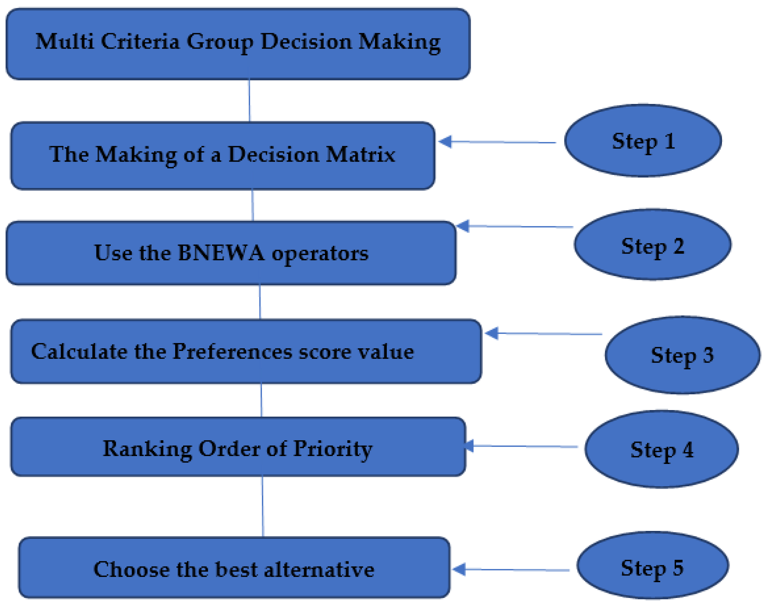
5. Multi-Criteria Group DM Problem Based on BN Einstein Aggregation Operators

This section includes a multi-criteria application based on BN Einstein aggregation operators (AOs), along with crisp numbers serving as attributes’ weights and BN numbers serving as attributes’ values.

5.1. Algorithm

Consider $G=\left\{G_1,G_2,\dots ,G_m\right\}$ to represent a collection of finite m alternatives, $L=\left\{L_1,L_2,L_3,\dots ,L_n\right\}$ to represent a collection of finite n attributes and $D^{}{=}_{}\left\{D_1,D_2,D_3,\dots ,D_k\right\}$ to be a finite number of k decision-makers. Suppose $\nu ={\left({\nu }_1,{\nu }_2,\dots ,{\nu }_n\right)}^T$ is the weighted vector for decision-makers $\overline{D^s}\left(s=1,2,3,\dots ,k-1,k\right),$ with ${\nu }_l\in \left[0{,}^{}1\right]$ and ${\displaystyle \sum _{l=1}^n}{\nu }_l=1$. Suppose $w={\left(w_1,w_2,w_3,\dots ,w_n\right)}^T$ is the weighted vector representing the set of attributes $L=\left\{L_1,L_2,L_3,\dots ,L_n\right\}$, with $w_l\in \left[0,1\right]$ and ${\displaystyle \sum _{l=1}^n}{w}_l=1$. The decision-maker assesses an option based on a set of criteria, the values of which are defined by BNVs. Let $u_{\stackrel{⌢}{i}\stackrel{⌢}{j}}^{\left(s\right)}={\left[\left({\Im }_{\stackrel{⌢}{i}\stackrel{⌢}{j}}^{+}{}_{},{{\rm I}}_{\stackrel{⌢}{i}\stackrel{⌢}{j}}^{+}{}^{},{ƒ}_{\stackrel{⌢}{i}\stackrel{⌢}{j}}^{+}{}_{},{\Im }_{\stackrel{⌢}{i}\stackrel{⌢}{j}}^{-}{}^{},{{\rm I}}_{\stackrel{⌢}{i}\stackrel{⌢}{j}}^{-}{,}_{}{ƒ}_{\stackrel{⌢}{i}\stackrel{⌢}{j}}^{-}\right)\right]}_{m\times n}$ be the decision matrices provided by an expert decision-maker, and $u_{\stackrel{⌢}{i}\stackrel{⌢}{j}}^{\left(s\right)}$ be a BNN for $L_{\stackrel{⌢}{i}}$ attribute associated with alternatives. We have ${\Im }_{\stackrel{⌢}{i}\stackrel{⌢}{j}}^{+},{{\rm I}}_{\stackrel{⌢}{i}\stackrel{⌢}{j}}^{+},{ƒ}_{\stackrel{⌢}{i}\stackrel{⌢}{j}}^{+},{\Im }_{\stackrel{⌢}{i}\stackrel{⌢}{j}}^{-},{{\rm I}}_{\stackrel{⌢}{i}\stackrel{⌢}{j}}^{-}$ and ${ƒ}_{\stackrel{⌢}{i}\stackrel{⌢}{j}}^{-}\in \left[0{,}^{}1\right]$ with condition $0\le {\Im }_{\stackrel{⌢}{i}\stackrel{⌢}{j}}^{+}+{{\rm I}}_{\stackrel{⌢}{i}\stackrel{⌢}{j}}^{+}{}^{}{+}_{}{ƒ}_{\stackrel{⌢}{i}\stackrel{⌢}{j}}^{+}{}^{}{+}_{}{\Im }_{\stackrel{⌢}{i}\stackrel{⌢}{j}}^{-}+{{\rm I}}_{\stackrel{⌢}{i}\stackrel{⌢}{j}}^{-}+{ƒ}_{\stackrel{⌢}{i}\stackrel{⌢}{j}}^{-}{}^{}{\le }_{}6$, where ${\stackrel{⌢}{i}}^{}{=}_{}1,2,3,\dots ,m-1,m$ and ${\stackrel{⌢}{j}}^{}{=}_{}1{,}^{}2,3,\dots ,n$. (Figure 1)

Step 1: Matrix construction (

Table 1. BN decision matrix by decision-maker D₁.

	L1	L2	L3	L4
G1	(0.2,0.6,0.5,−0.3,−0.9,−0.6)	(0.4,0.6,0.7,−0.5,−0.4,−0.3)	(0.8,0.3,0.5,−0.6,−0.1,−0.9)	(0.5,0.4,0.6,−0.8,−0.5,−0.4)
G2	(0.5,0.7,0.3,−0.8,−0.5,−0.7)	(0.3,0.4,0.6,−0.8,−0.7,−0.6)	(0.4,0.6,0.9,−0.5,−0.4,−0.5)	(0.3,0.8,0.9,−0.1,−0.4−0.3)
G3	(0.5,0.7,0.8,−0.4,−0.7,−0.4)	(0.3,0.7,0.7,−0.5,−0.3,−0.2)	(0.5,0.3,0.4,−0.6,−0.7,−0.9)	(0.4,0.6,0.5,−0.3,−0.5,−0.8)
G4	(0.8,0.5,0.4,−0.7,−0.6,−0.5)	(0.2,0.4,0.5,−0.8,−0.6,−0.3)	(0.3,0.7,0.4,−0.5,−0.7,−0.5)	(0.9,0.4,0.6,−0.5,−0.4,−0.7)

Table 2. BN decision matrix by decision-maker D₂.

	L1	L2	L3	L4
G1	(0.4,0.6,0.5,−0.7,−0.4,−0.8)	(0.5,0.4,0.6,−0.8,−0.5,−0.7)	(0.4,0.6,0.5,−0.4,−0.8,−0.5)	(0.5,0.6,0.3,−0.4,−0.6,−0.8)
G2	(0.4,0.7,0.5,−0.6,−0.3,−0.9)	(0.4,0.7,0.8,−0.3,−0.5,−0.4)	(0.2,0.5,0.7,−0.6,−0.5,−0.4)	(0.8,0.4,0.2,−0.8,−0.1,−0.4)
G3	(0.6,0.3,0.6,−0.3,−0.7,−0.8)	(0.6,0.4,0.6,−0.7,−0.5,−0.8)	(0.6,0.3,0.2,−0.1,−0.4,−0.7)	(0.5,0.6,0.7,−0.3,−0.5,−0.6)
G4	(0.2,0.3,0.4,−0.7,−0.6,−0.8)	(0.8,0.5,0.4,−0.7,−0.4,−0.6)	(0.8,0.4,0.5,−0.7,−0.5,−0.1)	(0.6,0.5,0.8,−0.7,−0.6,−0.4)

Table 3. BN decision matrix by decision-maker D₃.

	L1	L2	L3	L4
G1	(0.5,0.6,0.4,−0.7,−0.4,−0.3)	(0.2,0.5,0.6,−0.4,−0.7,−05)	(0.5,0.7,0.2,−0.9,−0.5,−0.3)	(0.5,0.6,0.3,−0.7,−0.5,−0.2)
G2	(0.9,0.2,0.4,−0.5,−0.4,−0.8)	(0.5,0.1,0.2,−0.9,−0.6,−0.4)	(0.1,0.4,0.8,−0.6,−0.5,−0.3)	(0.6,0.5,0.3,−0.9,−0.3,−0.5)
G3	(0.4,0.5,0.6,−0.1,−0.6,−0.5)	(0.3,0.4,0.8,−0.5,−0.4,−0.3)	(0.4,0.6,0.3,−0.4,−0.5,−0.3)	(0.5,0.4,0.9,−0.5,−0.4,−0.7)
G4	(0.1,0.4,0.5,−0.4,−0.8,−0.7)	(0.4,0.3,0.6,−0.2,−0.7,−0.5)	(0.7,0.5,0.6,−0.4,−0.3−0.9)	(0.1,0.5,0.7,−0.5,−0.8,−0.3)

) for decision-making $\overline{D^s}={\left[u_{\stackrel{⌢}{i}\stackrel{⌢}{j}}^{\left(s\right)}\right]}_{m\times n}\left(s=1,2,3,\dots ,k-1,k\right)$.

Step 2: Computing $BNEW{A}_{\nu }\left(r_{\stackrel{⌢}{i}1},r_{\stackrel{⌢}{i}2},\dots ,r_{\stackrel{⌢}{i}n}\right)$ (

Table 4. A collective BN decision matrix R.

	L1	L2
G1	(0.4234,0.6000,0.4581,−0.6501,−0.4842,−0.6306)	(0.3783,0.4568,0.6096,−0.5917,−0.5810,−0.5943)
G2	(0.6940,0.4453,0.4360,−0.5766,−0.3620,−0.8517)	(0.4219,0.3288,0.4750,−0.5426,−0.5640,−0.4224)
G3	(0.5161,0.4057,0.6187,−0.2024,−0.6627,−0.6704)	(0.4632,0.4251,0.6870,−0.5952,−0.4423,−0.6001)
G4	(0.2462,0.3555,0.4381,−0.5675,−0.6938,−0.7403)	(0.6286,0.4014,0.4839,−0.4527,−0.5567,−0.5351)
	L3	L4
G1	(0.4940,0.6011,0.3536,−0.5954,−0.6522,−0.4973)	(0.5000,0.5776,0.3233,−0.5453,−0.5520,−0.5868)
G2	(0.1818,0.4670,0.7589,−0.5895,−0.4905,−0.3718)	(0.6950,0.4726,0.2807,−0.7190,−0.2130,−0.4321)
G3	(0.5161,0.4021,0.2533,−0.2160,−0.4764,−0.6073)	(0.4905,0.5135,0.7552,−0.3708,−0.4614,−0.6659)
G4	(0.7293,0.4649,0.5274,−0.5482,−0.4504,−0.6005)	(0.4884,0.4893,0.7387,−0.5952,−0.6796,−0.3989)

) for every ${\stackrel{⌢}{i}}^{}{=}_{}1,2,3,\dots ,m$. $\begin{array}{l}{r}_{\stackrel{⌢}{i}}=\left({\Im }_{}{}_{\stackrel{⌢}{i}}^{+},{{\rm I}}^{}{{}_{\stackrel{⌢}{i}}^{+}}_{},{ƒ}^{}{{}_{\stackrel{⌢}{i}}^{+}}^{{}_{}},{\Im }^{}{}_{\stackrel{⌢}{i}}^{-},{{\rm I}}_{}{}_{\stackrel{⌢}{i}}^{-},{ƒ}_{\stackrel{⌢}{i}}^{-}\right)=\\ BNEW{A}_{\nu }\left(r_{\stackrel{⌢}{i}1},r_{\stackrel{⌢}{i}2},\dots ,r_{\stackrel{⌢}{i}n}\right)=\underset{l=1}{\overset{n}{\oplus }}\left({\nu }_l{r}_{il}\right)=\\ \left(\frac{{Ђ}_1-{Ђ}_2}{{Ђ}_1+{Ђ}_2},\frac{2{\zeta }_1}{{\zeta }_2+{\zeta }_1},\frac{2f_1}{f_2+f_1},\frac{-2{Ђ}_3}{{Ђ}_4+{Ђ}_3},-\frac{{\zeta }_3-{\zeta }_4}{{\zeta }_3+{\zeta }_4},-\frac{f_3-f_4}{f_3+f_4}\right)\end{array}$

Step 3: Computing the scores values $S\left(r_{\stackrel{⌢}{i}}\right)$.

Step 4: Various software systems are ranked for $BNEW{A}_{\nu }\left(u_{\stackrel{⌢}{i}1},u_{\stackrel{⌢}{i}2},\dots ,u_{\stackrel{⌢}{i}n}\right)$ in accordance with their scores.

Step 5: Picking the best option.

5.2. Illustrative Example

We believe that a medicine business company should hire a professional manager. For this reason, the organization formsa working group with three decision-makers in weighting vectors $\nu ={(0.1,0.5,0.4)}^T.$ When choosing the most knowledgeable management approach, there are various factors to evaluate, but in this situation, the committee just analyses the four criteriamentioned below, along with associated weighted vector $\nu ={(0.1,0.4,0.2,0.3)}^T.$ Four managers $G_j\left(j=1,2,3,4\right)$ will advance to the next round of the procedure after passing the first screening exam.

L₁: Salary;

L₂: Experience;

L₃: Working skill;

L₄: Dealing with public.

Step 1. Matrices construction for decisions.

Step 2: Compute $BNEW{A}_{\nu }\left(r_{\stackrel{⌢}{i}1},r_{\stackrel{⌢}{i}2},\dots ,r_{\stackrel{⌢}{i}n}\right)$

$$\begin{array}{c}{r}_{\stackrel{⌢}{i}}=\left({\Im }_{}{}_{\stackrel{⌢}{i}}^{+},{{\rm I}}^{}{}_{\stackrel{⌢}{i}}^{+},{ƒ}_{\stackrel{⌢}{i}}^{+},{\Im }^{}{}_{\stackrel{⌢}{i}}^{-},{{\rm I}}_{}{}_{\stackrel{⌢}{i}}^{-},{ƒ}_{\stackrel{⌢}{i}}^{-}\right)=\hfill \\ BNEW{A}_{\nu }\left(r_{\stackrel{⌢}{i}1},r_{\stackrel{⌢}{i}2},\dots ,r_{\stackrel{⌢}{i}n}\right)=\underset{l=1}{\overset{n}{\oplus }}\left({\nu }_l{r}_{il}\right)=\hfill \\ \left(\frac{{Ђ}_1-{Ђ}_2}{{Ђ}_1+{Ђ}_2},\frac{2{\zeta }_1}{{\zeta }_2+{\zeta }_1},\frac{2f_1}{f_2+f_1},\frac{-2{Ђ}_3}{{Ђ}_4+{Ђ}_3},-\frac{{\zeta }_3-{\zeta }_4}{{\zeta }_3+{\zeta }_4},-\frac{f_3-f_4}{f_3+f_4}\right) \hfill \end{array}$$

Step 3: Now, compute the scoring function of

$$\begin{array}{l}{r}_1=\left(0.3029,0.5336,0.4445,-0.5839,-0.4416,-0.4277\right),\\ r_2=\left(0.2934,0.4068,0.4501,-0.6059,-0.3806,-0.3667\right),\\ r_3=\left(0.3556,0.4435,0.5882,-0.3867,-0.3570,-0.4616\right),\\ r_4=\left(0.4670,0.4341,0.5578,-0.5236,-0.4085,-0.4405\right),\\ S\left(r_{\stackrel{⌢}{i}}\right)=\frac{1}{6}\left({\Im }^{+}+1-{{\rm I}}^{+}+1-{ƒ}^{+}+1+{\Im }^{-}-{{\rm I}}^{-}-{ƒ}^{-}\right), \\ S\left(r_1\right)=.4350,S\left(r_2\right)=0.4296,S\left(r_3\right)=.4593,S\left(r_4\right)=0.4668\end{array}$$

Step 4: We have arrived at a conclusion by calculating the scores:

$$G_4\succ G_3\succ G_1\succ G_2$$

Step 5: The best option is G₄.

6. Comparison

Different researchers have used a wide range of DM approaches so far. Chen et al. [28] used FSs, Atanassov [2] used IFSs, Zavadskas et al. [21] used NSs, Dubois et al. [34] used BFSsand Irfan et al. [25] used BNSs, among other study approaches.We employed Einstein operators to apply bipolarity to neutrosophic sets in this paper.

The aggregation operators in this study were broader and more versatile, representing an advantage of our proposed method, which led us to determine that G₄ was the best manager for the job.

7. Conclusions

The goal of this research was to look at different BN aggregation operators developed with the help of Einstein t-norms/t-conorms for multi-criteria community DM using BNVs as the criteria. The Einstein t-norm typically gives the same smooth approximations as the product and sum of an algebraic t-norm. Motivated by Einstein operations, we suggested bipolar neutrosophic Einstein aggregation operators for decision-making problems. To begin with, we looked at BN Einstein aggregation operators and the properties that they must have. Along with their attributes, these AOs were (BNEWA),(BNEOWA), (BNEHWA), (BNEWG), (BNEOWG)and (BNEHWG). Finally, we showed how to make multi-criteria decisions using such a framework. A descriptive case of manager selection was studied. The outcomes of the present paper show that the proposed approaches are accurate and practical when put into practice. We plan to extend the proposed approach to other domains and employ it in future research projects, such as pattern identification and risk analysis.

References

1. Zadeh, L.A. Fuzzy sets. Inf. Control. 1965, 8, 338–353. [Google Scholar] [CrossRef] [Green Version]
2. Atanassov, K.T. Intuitionistic fuzzy sets. Fuzzy Sets Syst. 1986, 20, 87–96. [Google Scholar] [CrossRef]
3. Smarandache, F. A Unifying Field in Logics Neutrosophy and Neutrosophic Probability, Set and Logic; American Research Press: Rehoboth, DE, USA, 1999. [Google Scholar]
4. Wang, H.; Smarandache, F.; Zhan, Y.; Sunderraman, R. Single valued neutrosophic sets. In Proceedings of the 10th 476 International Conference on Fuzzy theory and Technology, Salt Lake City, UT, USA, 21–26 July2005. [Google Scholar]
5. Ye, J. Multicriteria decision-making method using the correlation coefficient under single valued neutrosophic environment. Int. J. Gen. Syst. 2013, 42, 386–394. [Google Scholar] [CrossRef]
6. Wang, H.; Smarandache, F.; Zhan, Y.Q. Interval Neutrosophic Sets and Logic; Theory and Applications in Computing; Hexis: Phoenix, AZ, USA, 2005. [Google Scholar]
7. Yu, D.J. Group decision making based on generalized intuitionistic fuzzy prioritized geometric operator. Int. J. Intell. Syst. 2012, 27, 635–661. [Google Scholar] [CrossRef]
8. Shakeel, M.; Aslam, M.; Amin, N.; Jamil, M. Method of MAGDM based on Pythagorean trapezoidal uncertain linguistic hesitant fuzzy aggregation operatorwith Einstein operations. J. Intell. Fuzzy Syst. 2020, 38, 2211–2230. [Google Scholar] [CrossRef]
9. Wang, W.; Liu, X. Intuitionistic Fuzzy Geometric Aggregation Operators Based on Einstein Operations. Int. J. Intell. Syst. 2011, 26, 1049–1075. [Google Scholar] [CrossRef]
10. Xu, Z.S. Multi-person multi-attribute decision making models under intuitionistic fuzzy environment. Fuzzy Optim. Decis. Mak. 2007, 6, 221–236. [Google Scholar] [CrossRef]
11. Qun, W.; Peng, W.; Ligang, Z.; Huayou, C.; Xianjun, G. Some new Hamacher aggregation operators under single-valued neutrosophic 2-tuple linguistic environment and their applications to multi-attribute group decision making. Comput. Ind. Eng. 2018, 116, 144–162. [Google Scholar]
12. Hamacher, H. Uber logischeverknunpfungennunssharferAussagen und derenZugenhorigeBewetungsfunktione. In Progress in Cybernatics and Systems Research; Riccardi, K., Ed.; Hemisphere: Washington, DC, USA, 1978; Volume 3, pp. 276–288. [Google Scholar]
13. Xu, Z.S. Intuitionistic fuzzy aggregation operators. IEEE Trans. Fuzzy Syst. 2007, 15, 1179–1187. [Google Scholar]
14. Zhao, X.; Wei, G. Some intuitionistic fuzzy Einstein hybrid aggregation operators and their application to multiple attribute decision making. Knowl. Based Syst. 2013, 37, 472–479. [Google Scholar] [CrossRef]
15. Xu, Z.S.; Yager, R.R. Some geometric aggregation operators based on intuitionistic fuzzy sets. Int. J. Gen. Syst. 2006, 35, 417–433. [Google Scholar] [CrossRef]
16. Wang, W.; Liu, X. Intuitionistic Fuzzy Information Aggregation Using Einstein Operations. IEEE Trans. Fuzzy Syst. 2012, 20, 923–938. [Google Scholar] [CrossRef]
17. Chen, S.M. A new approach to handling fuzzy decision-making problems. IEEE Trans. Syst. ManCybern. 1998, 18, 1012–1016. [Google Scholar] [CrossRef]
18. Zhang, W.R. Bipolar fuzzy sets and relations: A computational frame work for cognitive modeling and multiagent decision analysis. In Proceedings of theNAFIPS/IFIS/NASA’94, the First International Joint Conference of The North American Fuzzy Information Processing Society Biannual Conference, The Industrial Fuzzy Control and Intelligence, San Antonio, TX, USA, 18–21 December 1994; pp. 305–309. [Google Scholar]
19. Zhang, W.R. Bipolar fuzzy sets. In Proceedings of the 1998 IEEE International Conference on Fuzzy Systems Proceedings, IEEE World Congress on Computational Intelligence (Cat. No.98CH36228), Anchorage, AK, USA, 4–9 May 1998; pp. 835–840. [Google Scholar]
20. Zhang, W.R.; Zhang, L. Bipolar logic and Bipolar fuzzy logic. Inf. Sci. 2004, 165, 265–287. [Google Scholar] [CrossRef]
21. Zavadskas, E.K.; Bausys, R.; Kaklauskas, A.; Ubarte, I.; Kuzminske, A.; Gudience, N. Sustainable market valuation of buildings by the single-valued neutrosophic MAMVA method. Appl. Soft Comput. 2017, 57, 74–87. [Google Scholar] [CrossRef] [Green Version]
22. Zhang, W.R. Bipolar quantum logic gates and quantum cellular combinatorics-a logical extension to quantum entanglement. J. QuantumInf. Sci. 2013, 3, 93–105. [Google Scholar] [CrossRef] [Green Version]
23. Gul, Z. Some Bipolar Fuzzy Aggregations Operators and Their Applications in Multicriteria Group Decision Making. Ph.D. Thesis, Hazara University, Mansehra, Pakistan, 2015. [Google Scholar]
24. Deli, I.; Subas, Y.; Smarandache, F.; Ali, M. Interval valued bipolar neutrosophic sets and their application in pattern recognition. Conference Paper. arXiv 2016, arXiv:289587637. [Google Scholar]
25. Deli, I.; Ali, M.; Smarandache, F. Bipolar neutrosophic sets and their application based on multi-criteria decision making problems. In Proceedings of the 2015 International Conference on Advanced Mechatronic System, Beijing, China, 22–24 August 2015. [Google Scholar]
26. Jamil, M.; Abdullah, S.; Khan, M.Y.; Smarandache, F.; Ghani, F. Application of the Bipolar NeutrosophicHamacher Averaging Aggregation Operators to Group Decision Making: An Illustrative Example. Symmetry 2019, 11, 698. [Google Scholar] [CrossRef] [Green Version]
27. Jamil, M.; Rahman, K.; Abdullah, S.; Khan, M.Y. The induced generalized interval-valued intuitionistic fuzzyeinstein hybrid geometric aggregation operator and their application to group decision-making. J. Intell. Fuzzy Syst. 2020, 38, 1737–1752. [Google Scholar] [CrossRef]
28. Fan, C.; Ye, J.; Fen, S.; Fan, E.; Hu, K. Multi-criteria decision-making method using heronian mean operators under a bipolar neutrosophic environment. Mathematics 2019, 7, 97. [Google Scholar] [CrossRef] [Green Version]
29. Abdullah, S.; Aslam, M.; Ullah, K. Bipolar fuzzy soft sets and its applications in decision making problem. J. Intell. Fuzzy Syst. 2014, 27, 729–742. [Google Scholar] [CrossRef] [Green Version]
30. Jafar, M.N.; Zia, M.; Saeed, A.; Yaqoob, M.; Habib, S. Aggregation operators of bipolar neutrosophic soft sets and it’s applications in auto car selection. Int. J. NeutrosophicSci. 2020, 9, 37–46. [Google Scholar]
31. Ali, M.; Smarandache, F. Complex neutrosophicset. NeuralComput. Applic 2017, 28, 1817–1834. [Google Scholar] [CrossRef]
32. Broumi, S.; Bakali, A.; Talea, M.; Smarandache, F. Bipolar complex neutrosophic sets and its application in decision making problem. In Studies in Fuzziness and Soft Computing; Springer: Berlin/Heidelberg, Germany, 2018; pp. 677–710. [Google Scholar]
33. Jamil, M.; Afzal, F.; Afzal, D.; Thapa, D.K.; Maqbool, A. Multicriteria Decision-Making Methods Using Bipolar NeutrosophicHamacher Geometric Aggregation Operators. J. Funct. Spaces 2022, 2022, 5052867. [Google Scholar]
34. Dubois, D.; Kaci, S.; Prade, H. Bipolarity in reasoning and decision, an introduction. Info. Process. Manag. Uncertain. 2004, 4, 959–966. [Google Scholar]
Figure 1. Flow Chart for MCGDM.
Applsci 12 10045 g001