Article

Reliability of Lower-Cost Sensors in the Analysis of Indoor Air Quality on Board Ships

1
Antwerp Maritime Academy, Noordkasteel-Oost 6, 2030 Antwerp, Belgium
2
Department of Mathematics, Computer Science, University of Antwerp, Middelheimlaan 1, 2020 Antwerp, Belgium
3
Flemish Institute for Technological Research (VITO), Boeretang 200, 2400 Mol, Belgium
*
Author to whom correspondence should be addressed.
Atmosphere 2022, 13(10), 1579; https://doi.org/10.3390/atmos13101579
Submission received: 1 September 2022 / Revised: 20 September 2022 / Accepted: 23 September 2022 / Published: 27 September 2022

Abstract

:
Air quality in and around ships is governed by a variety of pollution sources that are unique for the shipping context. This makes the living and working conditions on ships substantially different from situations in cities or inside buildings. To gain insight into these differences, information about trends and absolute pollutant amounts on board ships is needed. However, the installation of reference instruments to monitor NO2, NO, O3, particulate matter and other environmental parameters is often not possible because of their size, weight or because of safety reasons. For that reason, more compact devices incorporating a variety of sensors are a good alternative. However, the use of such sensors is only possible when their behaviour and performance in a shipping context are well understood. To study this context, we were allowed to compare sensor-based measurements performed on a 36-year old ship dedicated to near shore operations with measurements of reference-grade instruments. Additional behavioural information of sensors is obtained by measuring campaigns organized on several inland ships. This contribution demonstrates that trends registered by gas and particulate matter sensors are reliable but that insufficient detection limits, higher noise, imperfect calibration and sensor errors result in some reliability constraints.

1. Introduction

From the numerous studies about indoor air quality in buildings, it is known that building materials, adhesives and wood in furnishing [1,2,3], consumer products (e.g., cleaning products, personal care products), human presence (e.g., metabolic emissions) and occupants’ activity (e.g., cooking) release a variety of gases and/or particulate matter [4,5,6,7,8,9]. The outgassing and emission from these indoor sources increases the pollutant background concentration due to the infiltration of pollutants from outdoor sources. Therefore, indoor sources affect human health and contribute to indoor air quality [10,11]. Indoor air pollutants are also found in vehicles’ cabins (e.g., cars, trucks) [12,13,14,15], in airplanes [16,17,18] or ships [19,20,21,22,23,24]. The specific design of a vessel and the dedicated building materials might influence the occurrence and behaviour of indoor sources. In addition, ships are also pollution hotpots that affect their environment [25,26,27,28,29,30,31]. Examples of ship related pollution sources that are less common in and around buildings are pollutants emitted by the engine (e.g., fuel [22,23], exhaust gases [22,32,33], vapours escaping from fuel tanks during filling or heating), cargo vapours [34,35], cargo operations where gas might escape, or works on deck such as repainting the ship with solvent-based paints [36]. Moreover, ships spend a substantial amount of time in harbors where industrial activities generate elevated levels of pollution. Another example of outdoor sources are dredging activities where odorous compounds such as H2S may be released [37,38]. Such outdoor sources affect the air inside a ship through infiltration. Therefore, it is possible that the concentration range and the dynamics in the concentration trends are different from the ones that are found in buildings. Unfortunately, there is insufficient knowledge available about the impact of all these pollution sources on the indoor air quality. An additional difficulty in the evaluation of indoor air quality is that the crew both live and work on their ship and that each of these situations have to comply with different legislation [34].
Unfortunately, the organization of measuring campaigns to analyze indoor air quality on ships is not straightforward. Ships are moving objects that are ashore during short time windows. In addition, these time windows are usually not known long in advance, so researchers and their measuring instruments must be on standby before boarding. Besides the need for highly mobile instruments, the height difference between deck and shore must be surmounted (there is not always a crane available) and they must be brought to the proper room by passing small doors and steep staircases. In addition, the wiring of the instruments inside the confined rooms must not compromise the safety of the ship and the crew, and it should not disturb the work of the crew. Therefore, compact and lightweight instruments are recommended for measuring campaigns on board ships. Unfortunately, the reference measuring methods as described in air quality directive 2008/50/EC [39] require instruments that are rather bulky or heavy. In addition, many of these instruments only monitor a limited number of environmental parameters so that several instruments must be combined to obtain an overall picture. The measuring conditions on ships are more aggressive for the devices than measurements in, for example, buildings (e.g., probability of displacements when the ship is rolling, elevated corrosion risk due to salts, etc.). This means that the use of expensive reference equipment entails a higher risk for the research team.
A possible solution to the mentioned restrictions is to use compact instruments that are not only cheaper but that can also measure multiple environmental parameters simultaneously. Some define a low-cost sensor as <$100 and a low cost monitor consisting of one or more sensors and communication/data components as <$1000 [40]. This study monitors a large number of environmental parameters by combining many sensors. Some of these sensors are somewhat more expensive (<$500). Due to the many sensors, the monitoring system costs about $5000. Therefore, we denote the system as a lower-cost system. The possibilities of lower-cost sensors have already been explored during environmental studies [41], occupational fields [42,43,44] and indoor air analysis [45]. Besides other advantages, this technology allows for the in-house development of monitoring systems by combining several lower-cost sensors with communication/data components [40,46,47,48,49,50,51,52,53,54,55,56]. An important collateral gain of cheaper instruments is that it becomes affordable to simultaneously monitor multiple locations. The usefulness of sensors is usually assessed by comparing sensors and reference measurements in laboratory conditions where environmental parameters are changed in a controlled way [57,58]. An alternative comparative test is to perform co-location experiments nearby national air quality measuring stations where pollutants in the air are determined with sufficient accuracy [59,60,61]. Different kinds of calibration procedures can be applied on the parallel measurements performed in laboratory or in co-location [62,63,64], such as simple linear regression, multi-linear regression [65] or machine learning [66,67,68] methods. The laboratory and field measurements give a good insight in the reliability of sensors but they are inappropriate to evaluate the impact of the shipping context on sensor measurements. Instead, mobile reference devices must be brought to the desired site. Several solutions exist to make such reference devices mobile: a van where the reference devices are built [69,70], drones or airplanes that are sniffing exhaust fumes from ships [71,72], and the use of more compact higher quality monitoring systems (e.g., Model 202 Ozone Monitor of 2B Technologies, Boulder, CO, USA [73], ozonesonde [74] such as the one of EN-SCI, Westminster, CO, USA).
Despite the advantages and possibilities of lower-cost monitoring systems, it is striking that quite a few publications emphasize the (calibration) limitations and the performance problems of such sensors [75,76]. In contrast to this negative way of evaluating lower-cost sensors [76,77], this contribution focuses on how meaningful sensor measurements can be in a shipping context. With ‘meaningful’ we mean how much useful information can be extracted from sensor readings to evaluate air quality while operating in a real-world application. As long as the data are good enough for analysing air quality or to sustain decision making, such devices are useful even when the data of reference devices are of higher quality. In this contribution, the meaningfulness of sensor measurements is assessed by comparing them with other sensors or with reference measurements performed inside ships. To this end, the difficulties of on board reference measurements have been overcome and several measuring campaigns are organized on a 36-year old ship dedicated to near shore operations. The study shows that most of the tested sensors generate valuable information and that the environmental parameters show strong fluctuations. These fluctuations are not sensor errors but contain meaningful information about the shipping context. However, some environmental parameters could not be evaluated with lower-cost sensors.

2. Materials and Methods

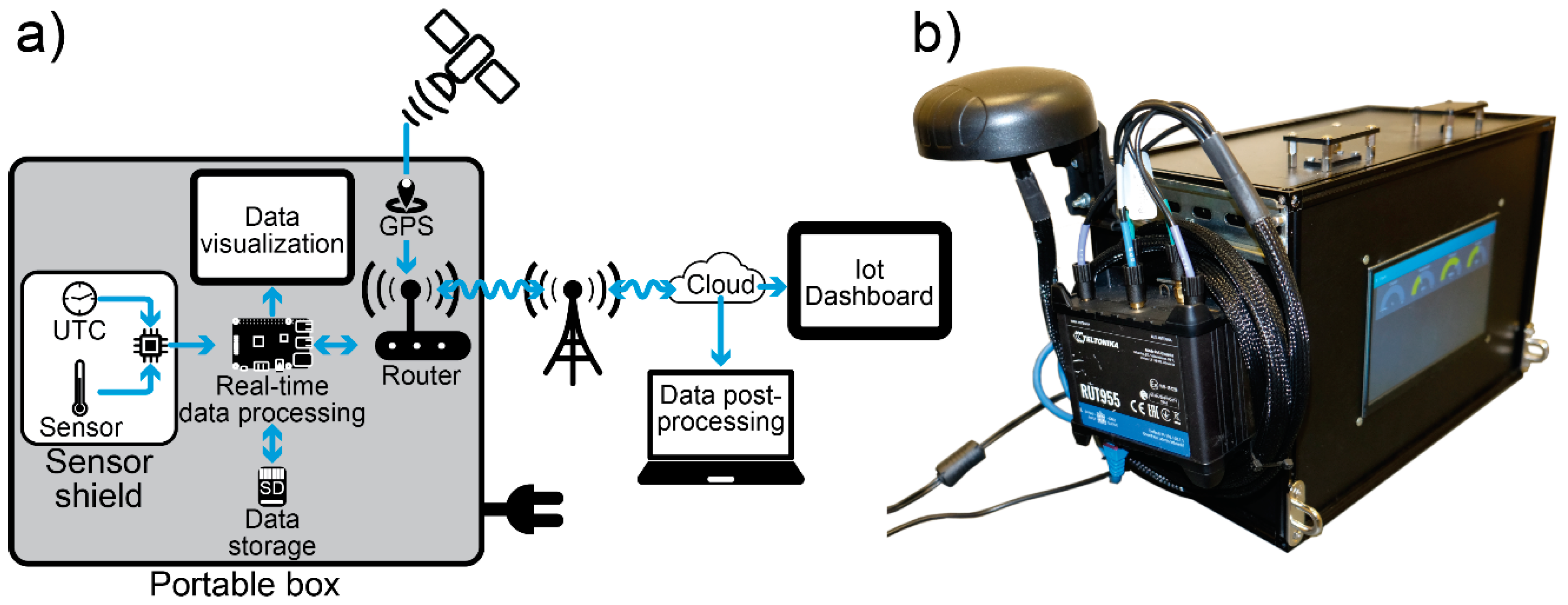
2.1. Lower-Cost Monitoring Device

The sensor box shown in Figure 1 contains a Poynting Puck antenna which is coupled to a Teltonika RUT955 router to assure the collection of georeferenced data. The router also establishes the connection with the Cloud. The single board computer (Raspberry Pi 3 Model B+) requests a measurement from the microprocessor (ATmega2560) on the PCB sensor shield. The microprocessor is connected to a real time clock (Maxim Integrated DS3231MZ+) and a wide range of sensors via a PCB. The board contains the following digital sensors: Sensirion SHT85(Temperature T, Relative humidity RH), E + E Elektronik EE894 (T, RH, pressure, CO2) and the OPC-N3 of Alphasense (PM1, PM2.5, PM10). The sensor shield also contains analog sensors whose signals are converted into digital signals via an ADC (Texas Instruments ADS1015): 6 B-type gas sensors of Alphasense (CO, NO2, O3, NO, H2S, SO2), the Alphasense PID-AH2 sensor for the total volatile organic compounds (TVOC) and the Alphasense VOC Metal Oxide sensors. The request of the single board computer to get the sensor values triggers the central microprocessor to perform a cycle in which all sensors are read for 10 times. That process is performed in a matter of milliseconds. The microprocessor calculates the average sensor readings and sends them to the single board computer. There, a Hampel filter treats the raw sensor signals in real time to suppress noise and replace outliers [78]. At the same time, a calibration function converts the raw signals into the corresponding physical values. The quantities obtained after calibration are also visualized on a screen that is incorporated in the side of the sensor box. For all sensors, laboratory-based calibration tests have shown a linear relationship between sensor readings and the corresponding physical values for measuring ranges expected in a shipping context. Although temperature and relative humidity in indoor conditions are more stable than for outdoor conditions, the measuring context still affects the calibration. Therefore, the calibration used cannot be considered as perfect. The sampling time is set to 3 min. This was initially considered as fast enough to monitor changes in a ship’s voyage and slow enough to give the single board computer the time to process all incoming data.

2.2. Measuring Campaigns

To gain insight about the performance of lower-cost sensors in the analysis of indoor air in ships, several studies were performed on a ship of 36 years old that is used for near-shore operations. The ship did not transport any cargo and always sailed on diesel. During the measuring campaign from 15–18 March 2021 in the engine room, the sensor box has been compared with the Airpointer, which was used as a reference-grade instrument. The Airpointer® (mlu-recordum Environmental Monitoring Solutions, Wiener Neustadt, Austria) is a heavy, large but transportable system equipped with several reference monitoring systems for NO, NOx, NO2 and O3. With the help of a crane, it was placed on the aft deck of the ship. The instrument was rolled into a room where the device was attached to a wall. With a sampling tube of about 30 m, air of the engine room could be sampled and analysed every minute. Prior to the measuring campaign, the instrument was calibrated in situ using gas bottles with a reference gas and with an ozone generator. The sensor box was installed next to the inlet of the sampling tube in the engine room. This means that both systems analyze exactly the same air.
During the measuring campaign of 24–26 November 2020 in the wheelhouse of the old ship, the sensor box was compared with a reference-grade instrument for particulate matter. The Grimm 11-D acted as a reference device for PM1, PM2.5 and PM10. It should be remarked that particulate matter in fresh ship engine exhaust are in the ultrafine particle size range (i.e., 1–400 nm) [79] and all particles below 253 nm are not observed by the instrument. In addition, Radiello radial-type diffusive samplers were used for the analysis of NO2 and SO2 (i.e., cylindrical cartridges RAD166 containing microporous polyethylene particles impregnated with triethanolamine). For a known period of time, the chemicals inside the cartridges selectively absorb the target gases. To avoid concentration gradients caused by the analytical method, the air nearby the diffusion tubes was forced to circulate using a small fan. The absorbed target gases are then extracted in a laboratory and quantified with ionic chromatography by following the Radiello specifications. A blank tube is always placed unopened at the measuring site and analysed together with the other tubes. No significant contamination has been found on the blanks.
In the period June–October 2021, the sensor boxes have been deployed in the kitchen, wheelhouse and/or engine room on four different inland ships. The inland ships are used for different types of activities. In that period, nine different time series have been collected. The time series have been used to evaluate the performance of the sensor boxes under different circumstances.

2.3. Performance Assessment of Sensors

The evaluation method used in this contribution analyzes sensors in a rather holistic way, looking not only at how well such sensors approach reference measurements but also at the reliability of the measured trends and the completeness of the analyses. Calibration issues are important, but it is not our aim to demonstrate that sensor measurements are of lower quality than reference measurements because this is already known, [59,63,80,81,82] as is often the reason for this [57,83]. Instead, we want to know whether sensors are good enough to underpin certain decisions that can improve indoor air quality on board ships. If this were the case, sensors could generate meaningful information. Therefore, it is more important to know why and when a sensor deviates from the reference measurements than how much it fails. The usefulness of sensor data is determined by the criteria given below. When a monitoring system satisfies the three criteria to some extent, then it is possible to build a decision support system around it [84,85].
Precision and accuracy of sensor measurements: For some parameters, it is possible to perform both reference and sensor measurements from the same room under real-world conditions at the same time. This makes it possible to visually compare both types of measurements with each other and to identify the reasons why a sensor fails to measure the parameter correctly. A good precision and accuracy of the measurements is important because it makes it possible to compare them with standards [86,87] and thresholds prescribed in legislation [88]. It gives an insight as to whether mitigation actions are needed;
Reliability of temporal trends: By conducting monitoring campaigns with reference and sensor based devices in the same room on board ships, it is possible to observe differences between both trends. The differences are related to the limitations of the sensor. When the reference instrument is not available, two sensors using different technologies to measure the same parameter can be compared instead. The similarities between them must be caused by the same air they are measuring and give an idea about the usefulness of the measurements. Trends give an insight in the moments of poorer air quality and are an important source of information about the behaviour of the hazards and thus about what kind of mitigation action is needed;
Completeness of the analysis: Missing a critical pollutant in the analysis might have a more substantial impact on the overall air quality assessment than, for example, imperfect calibration. That is why a large series of sensors have been used to measure the same indoor air on board ships. This allows us to find out which sensors are useful for such analyses and which are not.

3. Results

During the field-based comparative study performed in the engine room of the 36-year old ship, the trend and concentration of NO, NO2 and O3 could be studied in detail (see Figure 2). The trends in the reference measurements shown in Figure 2a suggest that the concentration of the pollutants fluctuate. For NO and NO2, the trend consists of a low but slowly fluctuating background concentration (NO: 0.5–2 ppb; NO2: 2–10 ppb) with top narrow peaks with variable heights. Some of these peaks are higher than 100 ppb. The trend of O3 consists of a background signal of 10–40 ppb with narrow valleys. The valley width varies between 2 and 24 min (average ± standard deviation: 12 ± 7 min). Some of the valleys are preceded by 1–9 min by an NO/NO2 peak. Most probably, the NO-peak triggers the following reaction with O3: NO + O3  NO2 + O2 [89]. When looking at the sensor measurements in Figure 2b, it is clear that the position of the tall NO and NO2 peaks coincide with the peaks measured with the reference instrument. The comparison indicates that the structure of the temporal trend as detected by the sensors is reliable. Despite some limitations as described in the list below, the three sensors are able to deliver meaningful information about the indoor air on board a ship:
Underestimation of peak maxima: The most obvious difference is that the NO and NO2 sensors severely underestimates the peak maxima. It is possible that the sensors are not able to follow the speed at which the concentration changes. Another explanation is that the linear calibration function as determined in laboratory conditions is affected by the context in which the measurements are performed. The underestimation introduces an uncertainty when the measurements are compared with the health-related threshold. This means that measurement uncertainties limit the extraction of useful information to some extent;
Undersampling: Since the peak widths are comparable with the sampling time of the sensor box (i.e., 3 min), such peaks are certainly affected by undersampling. A peak maximum between 2 sampling moments will be missed, resulting in an underestimation of the peak height. Some peaks only contain of 1 data point and may be wrongly considered as a spike by data cleaning methods (see for example also Figure 7b). Ship conditions are changing faster than originally expected and a sampling time of 1 min would have been more appropriate;
Worse detection limit: For NO, the low background signal and the smaller peaks detected by the Airpointer remain below the detection limit of the sensor and could not be detected (detection limit manufacture: ca. 15 ppb; detection limit based on peak detection: 20–40 ppb). However, the presence of large detectable peaks makes the NO-sensor usable to detect moments of worse indoor air quality;
Higher noise: For O3, the shape of the low-frequency background concentration is measured correctly but due to higher noise the valleys as detected by the Airpointer remain unresolved.
Figure 2. Pollutant concentration over time measured by the reference instrument and the sensor box of the same air in the engine room. The measuring campaign covers the period 15–18 March March 2021. Due to the complexity of the trends, it is impossible to superimpose sensor and reference measurements in a single graph; (a) 1-min data collected by the Airpointer containing reference instruments (NO2 and NO: chemiluminescence as prescribed by EN 14211:2005 [90]; O3: ultraviolet photometry as prescribed by EN 14625:2005 [91]); (b) 3-min data collected by the sensor box using electrochemical gas sensors of Alphasense.
Atmosphere 13 01579 g002
The sensor box also contains the Alphasense SO2 and H2S sensor so that their trends could be registered during monitoring campaigns (see Figure 3). Although SO2 is an important pollutant for seagoing vessels due to the sulphur content in heavy fuel [31,92], that sensor did not show meaningful trends during the organized monitoring campaigns. This must be due to the use of sulphur-poor diesel by the old ship and by the inland ships where measuring campaigns have been organized. The combined NO2-SO2 Radiello radial-type diffusive sampler was able to detect NO2 in several locations on the old ship, but SO2 remained below its detection limit of about 1 ppb for all locations. During one of the measuring campaigns, a reference monitoring system registered a background concentration of 1 ppb with peaks up to 7 ppb in a sleeping cabin. For the dredging sector, H2S is an important pollutant because it is produced in rotting processes in soils that are removed during dredging operations. Due to the problems described below, the trends observed cannot be considered as meaningful:
Signal is below detection limit: The SO2 and H2S indoor concentrations are close or below the detection limit of the sensors (detection limit according to manufacturer for SO2 and H2S is ca. 10 ppb). In addition, no concentration peaks exceeding the detection limit have been observed for these gases. Also in the city of Brussels, outdoor air at station 41R001 for 2021 is 0.8 ± 0.6 ppb with peak maxima below 5 ppb [93], suggesting that the pollutant concentration in outdoor air of a large city is systematically below detection limit of the sensor. The pollutant H2S is not measured by the national monitoring system in Belgium;
Dominant effect of cross-sensitivity: Although the pollutant concentration is below the detection limit, the sensor generates a trend (see Figure 3) that might be interpreted as a meaningful signal. However, these ‘trends’ may be caused by cross-sensitivity because the concentration of interfering gases such as NO2, NO or CO is higher than that of the target gas.
From analyses performed with Radiello™ diffusive samplers during other measuring campaigns on the ship, it is clear that the makeup of the mixture of organic compounds varies from location to location and with time (results not shown here). The variability in the mixture makes it impossible to calibrate the TVOC-sensors because the sensor has a different response to each compound. In addition, we had no reference-grade TVOC monitor at our disposal to perform an experiment in a co-location. Therefore, we have included a second TVOC-sensor in the sensor box. The PID and MOX sensors of the Alphasense measures the TVOC-content with a different technology. Since the sensors measure the TVOC-trend at the same location in an independent way, a correlation between both trends gives information about their meaningfulness. The trends of both sensors in Figure 4 show peaks on top of a background. Many of the peaks are in register and suggest that their variation is related to changes in the TVOC-concentration. However, the issues below limit the information that can be extracted from these trends:
Change in mixture makeup: Despite the fact that both sensors measure peaks at the same moment, at several occasions their response (red rectangle in Figure 4) to the same air is different. This must be due to a different response to a changing mixture of organic compounds. A series of TVOC sensors give an insight in the mixture makeup but it also complicates their calibration. Therefore, the raw signals in mV have been plotted in Figure 4;
Removal of sensor artefacts of the MOX-sensor: The heater temperature of the MOX-sensor is modulated between two temperatures to increase the selectivity. However, this modulation distorts the trend and this high frequency fluctuation must be removed by applying filters. Several types of filters have been tested but none of them could suppress the modulation completely. The filtering that has been applied resulted in ripples.
During another campaign in the old ship, a reference instrument was placed in the wheelhouse to analyse the trends and absolute values of particulate matter. The results of the reference measurements are shown in Figure 5a. In parallel, the Alphasense OPC-N3 sensor performed the same analysis (see Figure 5b). A first observation is that the peaks of both measuring systems are in register, meaning that they both observe the same trend. The trends in Figure 5a constitute tall peaks (PM10: peak width: 1–20 min; height 10–70 µg/m3) and broader peaks (PM10: width: 20–150 min; height: 20–50 µg/m3), superposed on a slowly fluctuating background signal (<1–10 µg/m3). The lower-cost sensor is able to measure both the background and peak contributions. This makes the OPC-N3 useful in the analysis of pollution sources affecting indoor air quality. However, some limitations have been noticed:
Invisible nanoparticles: Particulate matter in fresh ship engine exhaust are in the ultrafine particle size range (i.e., 1–400 nm) [79,94]. Since the OPC-N3 is only able to measure the presence of particles down to 350 nm, a large part of the ultrafine dust remains undetectable for the instrument. The reference instrument has a cut point of 253 nm and also suffers from this problem;
Elevated noise for PM10 measurements: The PM10 measurements with the OPC-N3 sensor tend to be more irregular than that of the reference instrument due to higher noise. In addition, PM10-phantom peaks appear to be present that are not observed by the reference instrument. For PM1 and PM2.5, the measurements by the sensor are less affected by noise and the sensor readings are more similar to the reference instrument;
Inconsistencies in the calibration: When comparing the PM1 measurements of both instruments, peaks are detected at the same moments. However, the sensor underestimates some peaks and overestimates others. For example, the peak ratio of the two larger peaks in the red rectangle in Figure 5 are clearly different (reference: 0.25; sensor: 0.5). In that period, both temperature and relative humidity can be considered as constant and cannot explain the difference in ratio. For the highest peak in the blue rectangle, the sensor registers a higher peak height than the reference instrument (20 vs. 34 µg/m3). There does not seem to be an obvious explanation for these variations in ratio. Although both instruments monitor air about 1 m apart, it is possible that the distribution of particulate matter in the wheelhouse is not homogenous.
The Alphasense OPC-N3 optical particle counter also sizes the particles in discrete bins. The mass concentrations PM1, PM2.5 and PM10 correspond with the first three bins, first six bins and first 12 bins, respectively. The number of detected particles in the first 12 bins are shown in Figure 6. The first 6 bins contain 99.997% of the detected particles, suggesting that PM10 should be close to the PM2.5 concentration. It should be remarked that aerosols from ship exhaust emissions contribute mostly to the fine fraction (PM1) and to a lesser extent to the medium-sized fraction (PM2.5) [95]. However, the OPC-N3 also registered elevated PM10 concentrations at some moments in time. For most of these moments, a higher number of particles have been detected in the bins of the smallest particles. In the higher bins, the number of particles remains low or even absent. Since the PM10 concentration is often higher than zero, an algorithm is most probably used that calculates the PM10 concentration (in µg/m3) by using the particle size distribution of the lower bins (expressed as number of particles). The impact of just a few larger particles on the particle size distribution might introduce random errors in the estimation of PM10.
In addition to the measuring campaigns on the old ship, other campaigns have been organized on various types of inland ships. During these campaigns, several sensor errors have been identified. The most remarkable errors are summarized in Figure 7 and described in the list below.
Saturation of the signal: The analog signal of the Alphasense CO-B4 sensor is a voltage and cannot exceed the input voltage of the power supply (i.e., 5 VDC) to which the sensor is connected. If the CO-concentration becomes too high, the signal will be saturated. Although the saturation level of c. 5 ppm is still below the non-occupational short-term exposure limits (around 6 ppm), the occupational TLV thresholds (about 10 ppm) and the occupational STEL thresholds (200 ppm), such high values were not expected in the wheelhouse. Arrow 1 shows the normal measurements of the working (i.e., signal proportional to the pollutant concentration) and auxiliary signal (i.e., background signal) of the sensor. Then, both electrodes are saturated but the auxiliary signal drops rather fast to 0 V (i.e., arrow 2). Arrow 3 shows the saturated signal of the working electrode while the auxiliary signal is zero. The peak width is about 30 min. After the occurrence of the peak, both electrodes have an output signal of 0 V (i.e., arrow 4). This behaviour suggests that the sensor has difficulties in measuring high concentrations and that time is needed before the sensor re-establishes its normal working conditions. It appears that in a shipping context a CO-sensor is needed that can measure a larger concentration range;
Undersampling: Figure 7b shows the occurrence of two peaks as measured by a reference system with a sampling time of 1 min and an NO2 sensor that is measuring every 3 min. For the sensor measurements, it is clear that some peaks appear as a spike (i.e., arrow 5). In this case, the spike contains meaningful information and should not be confused with an unwanted outlier;
Cross-sensitivity: The saturated CO-signal in Figure 7c is preceded by a tall TVOC-peak as detected by the Alphasense PID sensor. In that period, the working electrode of the NO sensor shows a negative peak (i.e., arrow 6). Since the CO concentration in air is so much higher than that of NO, the impact of CO on the NO-sensor due to cross-sensitivity becomes increasingly important. In the zone where the CO-signal is dropping, a small H2S and NO peak is observed. It is not clear whether these peaks have a physical meaning;
Interference: During one measuring campaign, the measured voltages of the gas sensors contain a substantial amount of noise (see arrow 7 in Figure 7d). For unknown reasons, that interference suddenly disappeared and all sensors started to work properly again.

4. Discussion and Conclusions

Real time indoor air quality monitoring in real-world situations has demonstrated that lower-cost sensors give meaningful information for NO2, NO, O3, CO, TVOC and PM trends on board ships. This means that a multi-sensor monitoring system is able to give a fairly complete analysis. From the parameters used, on some occasions the CO exceeded the concentration range of the sensor and, therefore, a sensor with a wider measuring range might be preferable. For SO2 and H2S, no valuable information could be obtained for ships burning low sulphur fuel due to an insufficient detection limit. However, the detection limit of the sensors is about 1 ppb and is lower than the non-occupational long-term threshold for human health (20–30 ppb). For the PM measurements, PM1 and PM2.5 appear to be more reliable than the PM10 measurements.
The time series shows the presence of many fluctuations and peaks. The trends and the position of the peaks in the time series of the pollutants analysed are in line with the reference measurements. This means that the peaks have physical meaning. A multi-sensor monitoring system is able to monitor trends in pollutant concentrations in a reliable way. However, the sensor measurements also show several limitations. For NO, the lower background concentrations and the smaller peaks could not be detected due to the insufficient low detection limit. Although a sampling time of 3 min appeared to be reasonable during the organization of the measuring campaigns, it became clear that some tall peaks might have a width of about 6 min. Such tall peaks appear in the time series as spikes of a single data point that might be confused with unwanted outliers by data cleaning methods. Therefore, a sampling time of 1 min would have been more appropriate.
The sensor measurements suffer from imperfect calibration. For example, the peak heights in the trends can be underestimated. This suggests that calibrations performed under laboratory conditions cannot be extrapolated in a simple way to the context of a ship. The O3 signal is determined by subtracting the NO2 signal from the OX signal and contains higher levels of noise than the other lower-cost gas sensors. As a result, the valleys as seen in the reference measurements could hardly be observed in the sensor signal. More elaborate studies are needed to further improve the calibration method and reduce the contribution of noise.
The sensor readings also suffer from other artefacts. One of the artefacts is that at elevated CO-concentrations, the signal of the working and auxiliary electrodes of the CO-sensor is incorrect. If an interfering gas in air is considerably higher in concentration than the concentration of the target gas, the impact of that gas due to cross-sensitivity will dominate the sensor reading. This might explain the variation in the H2S and SO2 trends. Cross-sensitivity can also induce negative peaks. Finally, considerable amounts of noise is sometimes picked up from the environment.

Author Contributions

B.L. and M.S. organized the installation of the reference monitoring systems on board of the ship. B.L. has built the sensor shield of the sensor box and has calibrated the sensors. G.C. was responsible for the software development to visualize the collected data and to generate the images. The paper is written by O.S. and reviewed/edited by W.J. Finally, O.S. is responsible for the conceptualization of the paper. All authors have read and agreed to the published version of the manuscript.

Funding

This research was funded by Flanders Innovation & Entrepreneurship (VLAIO), grant number HBC.2019.2033 and the APC was funded with the co-financing from the several participating organizations.

Institutional Review Board Statement

Not applicable.

Informed Consent Statement

Not applicable.

Data Availability Statement

All data used in this study are available upon request.

Acknowledgments

The authors thank Flanders Innovation & Entrepreneurship (VLAIO) for the financial support of the TETRA-project ELGAS (project number HBC.2019.2033). The authors also thank Joeri Verbiest and Lorenz Adriaensen of Karel de Grote University of Applied Sciences and Arts and the following organizations for their contribution in the project: Engine Deck Repair (EDR), Mediport, eu.reca, Kenniscentrum Binnenvaart Vlaanderen, De Vlaamse Waterweg, Jan De Nul, General Bunkering Services (GBS), AllThingsTalk, LCL, Telenet Group bvba and Atmosafe.

Conflicts of Interest

The authors declare no conflict of interest.

References

  1. Schieweck, A.; Salthammer, T. Emissions from Construction and Decoration Materials for Museum Showcases. Stud. Conserv. 2009, 54, 218–235. [Google Scholar] [CrossRef]
  2. Schieweck, A. Very Volatile Organic Compounds (VVOC) as Emissions from Wooden Materials and in Indoor Air of New Prefabricated Wooden Houses. Build. Environ. 2021, 190, 107537. [Google Scholar] [CrossRef]
  3. Zhao, Z.; Pei, Y.; Zhao, P.; Wu, C.; Qu, C.; Li, W.; Zhao, Y.; Liu, J. Characterizing Key Volatile Pollutants Emitted from Adhesives by Chemical Compositions, Odor Contributions and Health Risks. Molecules 2022, 27, 1125. [Google Scholar] [CrossRef] [PubMed]
  4. Tham, K.W. Indoor Air Quality and Its Effects on Humans—A Review of Challenges and Developments in the Last 30 Years. Energy Build. 2016, 130, 637–650. [Google Scholar] [CrossRef]
  5. Mannan, M.; Al-Ghamdi, S.G. Indoor Air Quality in Buildings: A Comprehensive Review on the Factors Influencing Air Pollution in Residential and Commercial Structure. Int. J. Environ. Res. Public. Health 2021, 18, 3276. [Google Scholar] [CrossRef]
  6. Saini, J.; Dutta, M.; Marques, G. A Comprehensive Review on Indoor Air Quality Monitoring Systems for Enhanced Public Health. Sustain. Environ. Res. 2020, 30, 6. [Google Scholar] [CrossRef]
  7. González-Martín, J.; Kraakman, N.J.R.; Pérez, C.; Lebrero, R.; Muñoz, R. A State–of–the-Art Review on Indoor Air Pollution and Strategies for Indoor Air Pollution Control. Chemosphere 2021, 262, 128376. [Google Scholar] [CrossRef]
  8. Farmer, D.K.; Vance, M.E.; Abbatt, J.P.D.; Abeleira, A.; Alves, M.R.; Arata, C.; Boedicker, E.; Bourne, S.; Cardoso-Saldaña, F.; Corsi, R.; et al. Overview of HOMEChem: House Observations of Microbial and Environmental Chemistry. Environ. Sci. Process. Impacts 2019, 21, 1280–1300. [Google Scholar] [CrossRef]
  9. Vardoulakis, S.; Giagloglou, E.; Steinle, S.; Davis, A.; Sleeuwenhoek, A.; Galea, K.S.; Dixon, K.; Crawford, J.O. Indoor Exposure to Selected Air Pollutants in the Home Environment: A Systematic Review. Int. J. Environ. Res. Public. Health 2020, 17, 8972. [Google Scholar] [CrossRef]
  10. Lee, K.K.; Bing, R.; Kiang, J.; Bashir, S.; Spath, N.; Stelzle, D.; Mortimer, K.; Bularga, A.; Doudesis, D.; Joshi, S.S.; et al. Adverse Health Effects Associated with Household Air Pollution: A Systematic Review, Meta-Analysis, and Burden Estimation Study. Lancet Glob. Health 2020, 8, e1427–e1434. [Google Scholar] [CrossRef]
  11. Stafoggia, M.; Oftedal, B.; Chen, J.; Rodopoulou, S.; Renzi, M.; Atkinson, R.W.; Bauwelinck, M.; Klompmaker, J.O.; Mehta, A.; Vienneau, D.; et al. Long-Term Exposure to Low Ambient Air Pollution Concentrations and Mortality among 28 Million People: Results from Seven Large European Cohorts within the ELAPSE Project. Lancet Planet. Health 2022, 6, e9–e18. [Google Scholar] [CrossRef]
  12. Barnes, N.; Ng, T.; Ma, K.; Lai, K. In-Cabin Air Quality during Driving and Engine Idling in Air-Conditioned Private Vehicles in Hong Kong. Int. J. Environ. Res. Public. Health 2018, 15, 611. [Google Scholar] [CrossRef] [PubMed]
  13. Tolis, E.I.; Karanotas, T.; Svolakis, G.; Panaras, G.; Bartzis, J.G. Air Quality into Cabin Environment of Different Passenger Cars: Effect of Car Usage, Fuel Type and Ventilation/Infiltration Conditions. Environ. Sci. Pollut. Res. 2021, 28, 51232–51241. [Google Scholar] [CrossRef] [PubMed]
  14. Xu, B.; Chen, X.; Xiong, J. Air Quality inside Motor Vehicles’ Cabins: A Review. Indoor Built Environ. 2018, 27, 452–465. [Google Scholar] [CrossRef]
  15. Cheng, X.; Tan, Z.; Wang, X.; Tay, R. Air Quality in a Commercial Truck Cabin. Transp. Res. Part Transp. Environ. 2006, 11, 389–395. [Google Scholar] [CrossRef]
  16. Dechow, M.; Nurcombe, C.A.H. Aircraft Environmental Control Systems. In Air Quality in Airplane Cabins and Similar Enclosed Spaces; Hocking, M., Ed.; The Handbook of Environmental Chemistry; Springer: Berlin/Heidelberg, Germany, 2005; Volume 4H, pp. 3–24. ISBN 978-3-540-25019-7. [Google Scholar]
  17. Golui, K.D. Air Quality in Airplane Cabins and Similar Enclosed Spaces. Available online: https://www.researchgate.net/publication/338528470_Air_Quality_in_Airplane_Cabins_and_Similar_Enclosed_Spaces (accessed on 23 September 2022).
  18. Hocking, M.B.; Hocking, D. Air Quality in Airplane Cabins and Similar Enclosed Spaces; Springer Science & Business Media: Berlin/Heidelberg, Germany, 2005; ISBN 978-3-540-25019-7. [Google Scholar]
  19. Kim, S.S.; Lee, Y.G. Field Measurements of Indoor Air Pollutant Concentrations on Two New Ships. Build. Environ. 2010, 45, 2141–2147. [Google Scholar] [CrossRef]
  20. Webster, A.D.; Reynolds, G.L. Indoor Air Quality on Passenger Ships. In Air Quality in Airplane Cabins and Similar Enclosed Spaces; Hocking, M., Ed.; The Handbook of Environmental Chemistry; Springer: Berlin/Heidelberg, Germany, 2005; Volume 4H, pp. 335–349. ISBN 978-3-540-25019-7. [Google Scholar]
  21. Strandberg, B.; Österman, C.; Koca Akdeva, H.; Moldanová, J.; Langer, S. The Use of Polyurethane Foam (PUF) Passive Air Samplers in Exposure Studies to PAHs in Swedish Seafarers. Polycycl. Aromat. Compd. 2022, 42, 448–459. [Google Scholar] [CrossRef]
  22. Langer, S.; Österman, C.; Strandberg, B.; Moldanová, J.; Fridén, H. Impacts of Fuel Quality on Indoor Environment Onboard a Ship: From Policy to Practice. Transp. Res. Part Transp. Environ. 2020, 83, 102352. [Google Scholar] [CrossRef]
  23. Langer, S.; Moldanová, J.; Österman, C. Influence of Fuel Change on Indoor Environmental Quality On-Board a Passenger Ferry. In Proceedings of the 14th International Conference of Indoor Air Quality and Climate, Ghent, Belgium, 4–8 July 2016; p. 9. [Google Scholar]
  24. Langer, S.; Moldanová, J.; Bloom, E.; Österman, C. Indoor Environment On-Board the Swedish Icebreaker Oden. In Proceedings of Indoor Air 2014; Indoor Air Technical Committee, Ed.; International Society for Indoor Air Quality and Climate (ISIAQ): Hong Kong, China, 2014; p. 8. [Google Scholar]
  25. Busch, D.; Krause, K. Air Quality on the Rhine and in the Inland Ports of Duisburg and Neuss. Immissionsschutz 2021, 26, 9. [Google Scholar] [CrossRef]
  26. Wang, X.; Shen, Y.; Lin, Y.; Pan, J.; Zhang, Y.; Louie, P.K.K.; Li, M.; Fu, Q. Atmospheric Pollution from Ships and Its Impact on Local Air Quality at a Port Site in Shanghai. Atmos. Chem. Phys. 2019, 19, 6315–6330. [Google Scholar] [CrossRef] [Green Version]
  27. Walker, T.R.; Adebambo, O.; Feijoo, M.C.D.A.; Elhaimer, E.; Hossain, T.; Edwards, S.J.; Morrison, C.E.; Romo, J.; Sharma, N.; Taylor, S.; et al. World Seas: An Environmental Evaluation Volume III: Ecological Issues and Environmental Impacts. In World Seas: An Environmental Evaluation; Academic Press: Cambridge, MA, USA, 2019; Volume 3, p. 26. [Google Scholar]
  28. Mueller, D.; Uibel, S.; Takemura, M.; Klingelhoefer, D.; Groneberg, D.A. Ships, Ports and Particulate Air Pollution—An Analysis of Recent Studies. J. Occup. Med. Toxicol. 2011, 6, 31. [Google Scholar] [CrossRef] [PubMed]
  29. IMO. Third IMO Greenhouse Gas Study 2014: Executive Summary and Final Report; International Maritime Organization: London, UK, 2015. [Google Scholar]
  30. Dabdub, D. Air Quality Impacts of Ship Emissions in the South Coast Air Basin of California; University of California: Irvine, CA, USA, 2008; p. 45. [Google Scholar]
  31. Zhao, J.; Wei, Q.; Wang, S.; Ren, X. Progress of Ship Exhaust Gas Control Technology. Sci. Total Environ. 2021, 799, 149437. [Google Scholar] [CrossRef] [PubMed]
  32. Lehtoranta, K.; Aakko-Saksa, P.; Murtonen, T.; Vesala, H.; Ntziachristos, L.; Rönkkö, T.; Karjalainen, P.; Kuittinen, N.; Timonen, H. Particulate Mass and Nonvolatile Particle Number Emissions from Marine Engines Using Low-Sulfur Fuels, Natural Gas, or Scrubbers. Environ. Sci. Technol. 2019, 53, 3315–3322. [Google Scholar] [CrossRef]
  33. Pillot, D.; Guiot, B.; Cottier, P.L.; Perret, P.; Tassel, P. Exhaust Emissions from In-Service Inland Waterways Vessels. In Proceedings of the TAP 2016, 21st International Transport and Air Pollution Conference, Lyon, France, 24–26 May 2016; Scienpress Ltd.: Lyon, France, 2016; Volume 6, pp. 205–225. [Google Scholar]
  34. Jacobs, W. Cargo Vapour Concentrations on Board Chemical Tankers in the Non-Cargo Area during Normal Operations. Ph.D. Thesis, Antwerp Maritime Academy, Antwerp, Belgium, 2019. [Google Scholar]
  35. Jacobs, W.; Reynaerts, C.; Andries, S.; Akker, S.; van den Moonen, N.; Lamoen, D. Analyzing the Dispersion of Cargo Vapors around a Ship’s Superstructure by Means of Wind Tunnel Experiments. J. Mar. Sci. Technol. 2016, 21, 758–766. [Google Scholar] [CrossRef]
  36. Celebi, U.B.; Vardar, N. Investigation of VOC Emissions from Indoor and Outdoor Painting Processes in Shipyards. Atmos. Environ. 2008, 42, 5685–5695. [Google Scholar] [CrossRef]
  37. Wang, X.; Guan, J.; Chattopadhyay, G.; Britton, G.; Panayotou, K.; Dickinson, T.; Stuetz, R.M. Odour and Odorant Emission Estimation of Dredged Sediment. In Proceedings of the A&WMA InternationaI Specialty Conference: Leapfrogging Opportunities for Air Quality Improvement, Xi’an, China, 10–14 May 2010; pp. 366–372. [Google Scholar]
  38. Wan, Y.; Ruan, X.; Wang, X.; Ma, Q.; Lu, X. Odour Emission Characteristics of 22 Recreational Rivers in Nanjing. Environ. Monit. Assess. 2014, 186, 6061–6081. [Google Scholar] [CrossRef] [PubMed]
  39. EU. Directive 2008/50/EC on Ambient Air Quality. Off. J. Eur. Union 2008, L152, 44. [Google Scholar]
  40. Morawska, L.; Thai, P.K.; Liu, X.; Asumadu-Sakyi, A.; Ayoko, G.; Bartonova, A.; Bedini, A.; Chai, F.; Christensen, B.; Dunbabin, M.; et al. Applications of Low-Cost Sensing Technologies for Air Quality Monitoring and Exposure Assessment: How Far Have They Gone? Environ. Int. 2018, 116, 286–299. [Google Scholar] [CrossRef]
  41. Snyder, E.G.; Watkins, T.H.; Solomon, P.A.; Thoma, E.D.; Williams, R.W.; Hagler, G.S.W.; Shelow, D.; Hindin, D.A.; Kilaru, V.J.; Preuss, P.W. The Changing Paradigm of Air Pollution Monitoring. Environ. Sci. Technol. 2013, 47, 11369–11377. [Google Scholar] [CrossRef]
  42. Fanti, G.; Spinazzè, A.; Borghi, F.; Rovelli, S.; Campagnolo, D.; Keller, M.; Borghi, A.; Cattaneo, A.; Cauda, E.; Cavallo, D.M. Evolution and Applications of Recent Sensing Technology for Occupational Risk Assessment: A Rapid Review of the Literature. Sensors 2022, 22, 4841. [Google Scholar] [CrossRef]
  43. Fanti, G.; Borghi, F.; Spinazzè, A.; Rovelli, S.; Campagnolo, D.; Keller, M.; Cattaneo, A.; Cauda, E.; Cavallo, D.M. Features and Practicability of the Next-Generation Sensors and Monitors for Exposure Assessment to Airborne Pollutants: A Systematic Review. Sensors 2021, 21, 4513. [Google Scholar] [CrossRef] [PubMed]
  44. Howard, J.; Murashov, V.; Cauda, E.; Snawder, J. Advanced Sensor Technologies and the Future of Work. Am. J. Ind. Med. 2022, 65, 3–11. [Google Scholar] [CrossRef]
  45. Ródenas García, M.; Spinazzé, A.; Branco, P.T.B.S.; Borghi, F.; Villena, G.; Cattaneo, A.; Di Gilio, A.; Mihucz, V.G.; Gómez Álvarez, E.; Lopes, S.I.; et al. Review of Low-Cost Sensors for Indoor Air Quality: Features and Applications. Appl. Spectrosc. Rev. 2022, 1–33. [Google Scholar] [CrossRef]
  46. Jo, J.; Jo, B.; Kim, J.; Kim, S.; Han, W. Development of an IoT-Based Indoor Air Quality Monitoring Platform. J. Sens. 2020, 2020, 8749764. [Google Scholar] [CrossRef]
  47. Suriano, D. A Portable Air Quality Monitoring Unit and a Modular, Flexible Tool for on-Field Evaluation and Calibration of Low-Cost Gas Sensors. HardwareX 2021, 9, e00198. [Google Scholar] [CrossRef] [PubMed]
  48. Hernández Rodríguez, E.; Schalm, O.; Martínez, A. Development of a Low-Cost Measuring System for the Monitoring of Environmental Parameters That Affect Air Quality for Human Health. ITEGAM-J. Eng. Technol. Ind. Appl. 2020, 6, 22–27. [Google Scholar] [CrossRef]
  49. Molka-Danielsen, J. Large Scale Integration of Wireless Sensor Network Technologies for Air Quality Monitoring at a Logistics Shipping Base. J. Ind. Inf. Integr. 2018, 9, 20–28. [Google Scholar] [CrossRef]
  50. Rodriguez-Vasquez, K.A.; Cole, A.M.; Yordanova, D.; Smith, R.; Kidwell, N.M. AIRduino: On-Demand Atmospheric Secondary Organic Aerosol Measurements with a Mobile Arduino Multisensor. J. Chem. Educ. 2020, 97, 838–844. [Google Scholar] [CrossRef]
  51. Alkandari, A.A.; Moein, S. Implementation of Monitoring System for Air Quality Using Raspberry PI: Experimental Study. Indones. J. Electr. Eng. Comput. Sci. 2018, 10, 43. [Google Scholar] [CrossRef]
  52. Gunawan, T.S.; Saiful Munir, Y.M.; Kartiwi, M.; Mansor, H. Design and Implementation of Portable Outdoor Air Quality Measurement System Using Arduino. Int. J. Electr. Comput. Eng. 2018, 8, 280. [Google Scholar] [CrossRef]
  53. Cross, E.S.; Williams, L.R.; Lewis, D.K.; Magoon, G.R.; Onasch, T.B.; Kaminsky, M.L.; Worsnop, D.R.; Jayne, J.T. Use of Electrochemical Sensors for Measurement of Air Pollution: Correcting Interference Response and Validating Measurements. Atmos. Meas. Tech. 2017, 10, 3575–3588. [Google Scholar] [CrossRef] [Green Version]
  54. Narayana, M.V.; Jalihal, D.; Nagendra, S.M.S. Establishing A Sustainable Low-Cost Air Quality Monitoring Setup: A Survey of the State-of-the-Art. Sensors 2022, 22, 394. [Google Scholar] [CrossRef] [PubMed]
  55. Abraham, S.; Li, X. A Cost-Effective Wireless Sensor Network System for Indoor Air Quality Monitoring Applications. Procedia Comput. Sci. 2014, 34, 165–171. [Google Scholar] [CrossRef]
  56. Panaitescu, M.; Panaitescu, F.V.; Dumitrescu, M.V.; Panaitescu, V.N. The Impact of Quality Air in The Engine Room on the Crew. TransNav Int. J. Mar. Navig. Saf. Sea Transp. 2019, 13, 409–414. [Google Scholar] [CrossRef]
  57. Samad, A.; Obando Nuñez, D.R.; Solis Castillo, G.C.; Laquai, B.; Vogt, U. Effect of Relative Humidity and Air Temperature on the Results Obtained from Low-Cost Gas Sensors for Ambient Air Quality Measurements. Sensors 2020, 20, 5175. [Google Scholar] [CrossRef]
  58. Wei, P.; Ning, Z.; Ye, S.; Sun, L.; Yang, F.; Wong, K.; Westerdahl, D.; Louie, P. Impact Analysis of Temperature and Humidity Conditions on Electrochemical Sensor Response in Ambient Air Quality Monitoring. Sensors 2018, 18, 59. [Google Scholar] [CrossRef]
  59. Wahlborg, D.; Björling, M.; Mattsson, M. Evaluation of Field Calibration Methods and Performance of AQMesh, a Low-Cost Air Quality Monitor. Environ. Monit. Assess. 2021, 193, 251. [Google Scholar] [CrossRef]
  60. Mijling, B.; Jiang, Q.; de Jonge, D.; Bocconi, S. Field Calibration of Electrochemical NO2 Sensors in a Citizen Science Context. Atmos. Meas. Tech. 2018, 11, 1297–1312. [Google Scholar] [CrossRef]
  61. Gonzalez, A.; Boies, A.; Swason, J.; Kittelson, D. Field Calibration of Low-Cost Air Pollution Sensors. Atmos. Meas. Tech. Discuss. 2019, 19, 1–7. [Google Scholar]
  62. Arroyo, P.; Gómez-Suárez, J.; Suárez, J.I.; Lozano, J. Low-Cost Air Quality Measurement System Based on Electrochemical and PM Sensors with Cloud Connection. Sensors 2021, 21, 6228. [Google Scholar] [CrossRef]
  63. Bigi, A.; Mueller, M.; Grange, S.K.; Ghermandi, G.; Hueglin, C. Performance of NO, NO2 Low Cost Sensors and Three Calibration Approaches within a Real World Application. Atmos. Meas. Tech. 2018, 11, 3717–3735. [Google Scholar] [CrossRef]
  64. Aguiar, E.F.K.; Roig, H.L.; Mancini, L.H.; Carvalho, E.N.C.B. de Low-Cost Sensors Calibration for Monitoring Air Quality in the Federal District—Brazil. J. Environ. Prot. 2015, 6, 173–189. [Google Scholar] [CrossRef] [Green Version]
  65. Ionascu, M.-E.; Castell, N.; Boncalo, O.; Schneider, P.; Darie, M.; Marcu, M. Calibration of CO, NO2, and O3 Using Airify: A Low-Cost Sensor Cluster for Air Quality Monitoring. Sensors 2021, 21, 7977. [Google Scholar] [CrossRef] [PubMed]
  66. Zimmerman, N.; Presto, A.A.; Kumar, S.P.N.; Gu, J.; Hauryliuk, A.; Robinson, E.S.; Robinson, A.L.; Subramanian, R. A Machine Learning Calibration Model Using Random Forests to Improve Sensor Performance for Lower-Cost Air Quality Monitoring. Atmos. Meas. Tech. 2018, 11, 291–313. [Google Scholar] [CrossRef]
  67. Smith, K.R.; Edwards, P.M.; Ivatt, P.D.; Lee, J.D.; Squires, F.; Dai, C.; Peltier, R.E.; Evans, M.J.; Sun, Y.; Lewis, A.C. An Improved Low-Power Measurement of Ambient NO2 and O3 Combining Electrochemical Sensor Clusters and Machine Learning. Atmos. Meas. Tech. 2019, 12, 1325–1336. [Google Scholar] [CrossRef]
  68. Wijeratne, L.O.H.; Kiv, D.R.; Aker, A.R.; Talebi, S.; Lary, D.J. Using Machine Learning for the Calibration of Airborne Particulate Sensors. Sensors 2019, 20, 99. [Google Scholar] [CrossRef]
  69. Drewnick, F.; Böttger, T.; von der Weiden-Reinmüller, S.-L.; Zorn, S.R.; Klimach, T.; Schneider, J.; Borrmann, S. Design of a Mobile Aerosol Research Laboratory and Data Processing Tools for Effective Stationary and Mobile Field Measurements. Atmos. Meas. Tech. 2012, 5, 1443–1457. [Google Scholar] [CrossRef]
  70. Borrego, C.; Costa, A.M.; Ginja, J.; Amorim, M.; Coutinho, M.; Karatzas, K.; Sioumis, T.; Katsifarakis, N.; Konstantinidis, K.; De Vito, S.; et al. Assessment of Air Quality Microsensors versus Reference Methods: The EuNetAir Joint Exercise. Atmos. Environ. 2016, 147, 246–263. [Google Scholar] [CrossRef]
  71. Beecken, J.; Mellqvist, J.; Salo, K.; Ekholm, J.; Jalkanen, J.-P. Airborne Emission Measurements of SO2, NOx and Particles from Individual Ships Using a Sniffer Technique. Atmos. Meas. Tech. 2014, 7, 1957–1968. [Google Scholar] [CrossRef]
  72. Anand, A.; Wei, P.; Gali, N.K.; Sun, L.; Yang, F.; Westerdahl, D.; Zhang, Q.; Deng, Z.; Wang, Y.; Liu, D.; et al. Protocol Development for Real-Time Ship Fuel Sulfur Content Determination Using Drone Based Plume Sniffing Microsensor System. Sci. Total Environ. 2020, 744, 140885. [Google Scholar] [CrossRef]
  73. Sagona, J.A.; Weisel, C.P.; Meng, Q. Accuracy and Practicality of a Portable Ozone Monitor for Personal Exposure Estimates. Atmos. Environ. 2018, 175, 120–126. [Google Scholar] [CrossRef]
  74. Lindqvist, F. A Differential Galvanic Atmospheric Ozone Monitor. Analyst 1972, 97, 549. [Google Scholar] [CrossRef] [PubMed]
  75. Concas, F.; Mineraud, J.; Lagerspetz, E.; Varjonen, S.; Liu, X.; Puolamäki, K.; Nurmi, P.; Tarkoma, S. Low-Cost Outdoor Air Quality Monitoring and Sensor Calibration: A Survey and Critical Analysis. ACM Trans. Sens. Netw. 2021, 17, 1–44. [Google Scholar] [CrossRef]
  76. Venkatraman Jagatha, J.; Klausnitzer, A.; Chacón-Mateos, M.; Laquai, B.; Nieuwkoop, E.; van der Mark, P.; Vogt, U.; Schneider, C. Calibration Method for Particulate Matter Low-Cost Sensors Used in Ambient Air Quality Monitoring and Research. Sensors 2021, 21, 3960. [Google Scholar] [CrossRef] [PubMed]
  77. Artinano, B.; Narros, A.; Diaz, E.; Gomez, F.J.; Borge, R. Low-Cost Sensors for Urban Air Quality Monitoring: Preliminary Laboratory and in-Field Tests within the TECNAIRE-CM Project. In Proceedings of the 2019 5th Experiment International Conference (exp.at’19), Funchal, Portugal, 12–14 June 2019; IEEE: Funchal, Portugal, 2019; pp. 462–466. [Google Scholar]
  78. Pearson, R.K.; Neuvo, Y.; Astola, J.; Gabbouj, M. Generalized Hampel Filters. EURASIP J. Adv. Signal Process. 2016, 2016, 87. [Google Scholar] [CrossRef]
  79. Kuittinen, N.; Jalkanen, J.-P.; Alanen, J.; Ntziachristos, L.; Hannuniemi, H.; Johansson, L.; Karjalainen, P.; Saukko, E.; Isotalo, M.; Aakko-Saksa, P.; et al. Shipping Remains a Globally Significant Source of Anthropogenic PN Emissions Even after 2020 Sulfur Regulation. Environ. Sci. Technol. 2021, 55, 129–138. [Google Scholar] [CrossRef] [PubMed]
  80. Lewis, A.C.; Lee, J.D.; Edwards, P.M.; Shaw, M.D.; Evans, M.J.; Moller, S.J.; Smith, K.R.; Buckley, J.W.; Ellis, M.; Gillot, S.R.; et al. Evaluating the Performance of Low Cost Chemical Sensors for Air Pollution Research. Faraday Discuss. 2016, 189, 85–103. [Google Scholar] [CrossRef]
  81. Li, H.; Zhu, Y.; Zhao, Y.; Chen, T.; Jiang, Y.; Shan, Y.; Liu, Y.; Mu, J.; Yin, X.; Wu, D.; et al. Evaluation of the Performance of Low-Cost Air Quality Sensors at a High Mountain Station with Complex Meteorological Conditions. Atmosphere 2020, 11, 212. [Google Scholar] [CrossRef]
  82. Kang, Y.; Aye, L.; Ngo, T.D.; Zhou, J. Performance Evaluation of Low-Cost Air Quality Sensors: A Review. Sci. Total Environ. 2022, 818, 151769. [Google Scholar] [CrossRef]
  83. Tagle, M.; Rojas, F.; Reyes, F.; Vásquez, Y.; Hallgren, F.; Lindén, J.; Kolev, D.; Watne, Å.K.; Oyola, P. Field Performance of a Low-Cost Sensor in the Monitoring of Particulate Matter in Santiago, Chile. Environ. Monit. Assess. 2020, 192, 171. [Google Scholar] [CrossRef]
  84. Schalm, O.; Cabal, A.; Anaf, W.; Leyva Pernia, D.; Callier, J.; Ortega, N. A Decision Support System for Preventive Conservation: From Measurements towards Decision Making. Eur. Phys. J. Plus 2019, 134, 74. [Google Scholar] [CrossRef]
  85. Anaf, W.; Leyva Pernia, D.; Schalm, O. Standardized Indoor Air Quality Assessments as a Tool to Prepare Heritage Guardians for Changing Preservation Conditions Due to Climate Change. Geosciences 2018, 8, 276. [Google Scholar] [CrossRef] [Green Version]
  86. Carro, G.; Schalm, O.; Jacobs, W.; Demeyer, S. Exploring Actionable Visualizations for Environmental Data: Air Quality Assessment of Two Belgian Locations. Environ. Model. Softw. 2022, 147, 105230. [Google Scholar] [CrossRef]
  87. Abdul-Wahab, S.A.; Chin Fah En, S.; Elkamel, A.; Ahmadi, L.; Yetilmezsoy, K. A Review of Standards and Guidelines Set by International Bodies for the Parameters of Indoor Air Quality. Atmos. Pollut. Res. 2015, 6, 751–767. [Google Scholar] [CrossRef]
  88. Nazarenko, Y.; Pal, D.; Ariya, P.A. Air Quality Standards for the Concentration of Particulate Matter 2.5, Global Descriptive Analysis. Bull. World Health Organ. 2021, 99, 125D–137D. [Google Scholar] [CrossRef]
  89. Leighton, P.A. Photochemistry of Air Pollution. In Physical Chemistry; Academic Press: New York, NY, USA, 1961; ISBN 978-0-12-442250-6. [Google Scholar]
  90. European Norm EN 14211:2012; Ambient Air—Standard Method for the Measurement of the Concentration of Nitrogen Dioxide and Nitrogen Monoxide by Chemiluminescence. European Committee for Standardization: Brussels, Belgium, 2012.
  91. European Norm EN 14625:2012; Ambient Air—Standard Method for the Measurement of the Concentration of Ozone by Ultraviolet Photometry. European Committee for Standardization: Brussels, Belgium, 2012.
  92. Vedachalam, S.; Baquerizo, N.; Dalai, A.K. Review on Impacts of Low Sulfur Regulations on Marine Fuels and Compliance Options. Fuel 2022, 310, 122243. [Google Scholar] [CrossRef]
  93. Belgian Interregional Environment Agency (IRCEL—CELINE—English. Available online: https://www.irceline.be/en/front-page?set_language=en (accessed on 18 May 2022).
  94. Alanen, J.; Isotalo, M.; Kuittinen, N.; Simonen, P.; Martikainen, S.; Kuuluvainen, H.; Honkanen, M.; Lehtoranta, K.; Nyyssönen, S.; Vesala, H.; et al. Physical Characteristics of Particle Emissions from a Medium Speed Ship Engine Fueled with Natural Gas and Low-Sulfur Liquid Fuels. Environ. Sci. Technol. 2020, 54, 5376–5384. [Google Scholar] [CrossRef]
  95. Bencs, L.; Horemans, B.; Buczyńska, A.J.; Deutsch, F.; Degraeuwe, B.; Van Poppel, M.; Van Grieken, R. Seasonality of Ship Emission Related Atmospheric Pollution over Coastal and Open Waters of the North Sea. Atmos. Environ. X 2020, 7, 100077. [Google Scholar] [CrossRef]
Figure 1. Overview of the sensor box. (a) General architecture of the sensor box where all sensors are attached to a sensor shield and that communicates with the Raspberry Pi; (b) Photo of the sensor box with the router and the screen incorporated in the side of the sensor box.
Atmosphere 13 01579 g001
Figure 3. Concentration of SO2 and H2S over time in the engine room during the same measuring campaign as shown in Figure 2. The 3-min data give the false impression of a meaningful trend. The measured concentrations with a faint variation between 0 and 2 ppb are close to the detection limit of the sensor.
Atmosphere 13 01579 g003
Figure 4. Measured TVOC-signal in mV over time and measured in the engine room during the same campaign as in Figure 2 and Figure 3. The trends are measured with a PID and MOX-sensor. The signal of the MOX-sensor is smoothed by a seven-point central moving median followed by a seven-point central moving average. The scale for MOX raw and MOX smoothed is different because the Y-axis of MOX raw is affected by the amplitude of the high frequency fluctuation. The red box is a detail where the peak ratios are different for PID and MOX sensor.
Atmosphere 13 01579 g004
Figure 5. Measured concentration of particulate matter in the wheelhouse of the old ship over time as determined with a high-end and low-cost optical particle counter monitoring. The measuring campaign covered the period 24–26 November 2020; (a) Reference measurements performed with the Grimm; (b) Measurements performed in the same room with the sensor box containing the Alphasense OPC-N3 sensor. The peak ratio in the red rectangle as determined by the 2 instruments are different. For the blue rectangle, the peak height of the largest peak as measured by the sensor is higher than for the reference measurement.
Atmosphere 13 01579 g005
Figure 6. Number of particles in the first 12 size bins as detected by the OPC-N3 sensor over time during the same monitoring campaign as the measurements in Figure 5. The discrete size bins give an insight into the particle size distribution.
Atmosphere 13 01579 g006
Figure 7. Raw sensor readings over time for the CO-B4 and NO2-B43F sensors and some sensor errors identified during a variety of monitoring campaigns. The signal of the working electrode is abbreviated as WE and of the auxiliary electrode as AUX; (a) A situation where the working electrode of the CO-sensor is saturated; (b) A situation where a peak consists of only one data point; (c) Situation of cross-sensitivity where NO shows a negative peak; (d) Situation where the environment creates noise in the WE and AUX signals and where this interference stops at some point.
Atmosphere 13 01579 g007
Publisher’s Note: MDPI stays neutral with regard to jurisdictional claims in published maps and institutional affiliations.

