
Optimizing Portfolio Risk of Cryptocurrencies Using Data-Driven Risk Measures
1
Department of Statistics, University of Manitoba, Winnipeg, MB R3T 2N2, Canada
2
Department of Computer Science, University of Manitoba, Winnipeg, MB R3T 2N2, Canada
*
Authors to whom correspondence should be addressed.
†
These authors contributed equally to this work.
J. Risk Financial Manag. 2022, 15(10), 427; https://doi.org/10.3390/jrfm15100427
Submission received: 19 August 2022
/
Revised: 5 September 2022
/
Accepted: 11 September 2022
/
Published: 25 September 2022
(This article belongs to the Special Issue Econometrics of Financial Models and Market Microstructure)
Abstract
:Portfolio risk management plays an important role in successful investments. Portfolio standard deviation, value-at-risk, expected shortfall, and maximum absolute deviation are widely used portfolio risk measures. However, the existing portfolio risk measures are vulnerable to larger skewness and kurtosis of the asset returns. Moreover, the traditional assumption of normality of the portfolio returns leads to the underestimation of portfolio risk. Cryptocurrencies are a decentralized digital medium of exchange. In contrast to physical money, cryptocurrency payments exist purely as digital entries on an online ledger called blockchain that describe specific transactions. Due to the high volume and high frequency of cryptocurrency transactions, risk forecasting using daily data is not enough, and a high-frequency analysis is required. High-frequency data reveal a very high excess kurtosis and skewness for returns of cryptocurrencies. In order to incorporate larger skewness and kurtosis of the cryptocurrencies, a data-driven portfolio risk measure is minimized to obtain the optimal portfolio weights. A recently proposed data-driven volatility forecasting approach with daily data are used to study risk forecasting for cryptocurrencies with high-frequency (hourly) big data. The paper emphasizes the superiority of portfolio selection of cryptocurrencies by minimizing the recently proposed risk measure over the traditional minimum variance portfolio.
1. Introduction and Motivation
Portfolio risk management plays an important role in successful investments. Following the global financial crisis in 2008 (see Appel and Grabinski 2011 for more details), financial markets are faced with a need for implementing sustainable forecasting models incorporating market risks. Some studies (Klinkova and Grabinski 2017) suggest that investing (betting) on unpredictable stock prices is identical to gambling. Employing volatility, value-at-risk (VaR), and conditional value-at-risk (CVaR) in the decision-making process of capital allocation helps to avoid the future risk of financial failures. A Basel III monitoring report by the Basel Committee on Banking Supervision in 2021 The Bank for International Settlements (2021) requires financial institutions to use more complex credit scoring models for efficient capital allocation and enhanced risk management.
A cryptocurrency is a digital form of money. Cryptocurrencies derive their value purely from the trust that is placed on them, and they are not backed by any commodity, such as gold or silver. The first cryptocurrency, Bitcoin, was founded in 2009 by Satoshi Nakamoto (a pseudonym) defining it as a “Peer-to-Peer (P2P) Electronic Cash System” Nakamoto (2008). Compared to the traditional systems which utilize a client–server, Bitcoin can be transferred through a P2P network from one user to other. This provides higher security compared to the traditional systems as it does depend on intermediaries and their central servers. The investments incorporating cryptocurrencies in their portfolios saw a rise during the year 2017 when Bitcoin started gaining significant value and popularity. However, despite high returns, it has also led to high risk in portfolios due to high skepticism about the widespread adoption of cryptocurrencies. Studies have been carried out for further comparison of cryptocurrencies with other portfolios such as stocks, currencies, and commodities Ma et al. (2020).
Recent studies in the area of computational finance have identified the negative effect of high kurtosis of the returns on traditional approaches Thavaneswaran et al. (2019, 2020); Liang et al. (2020). Furthermore, the normality assumption of returns leads to the underestimation of risks. This is due to the fact that the distributions of most returns tend to be not normal and have heavy or fat tails that tend to be skewed. That is, the traditional assumption of normality of the portfolio returns leads to underestimation of portfolio risk. It is also important to point out that, even though a random variable has a Gaussian-like distribution, the standard deviation may not be equal to sigma because, in many cases, random variables do not take values from negative infinity to positive infinity. Thus, drawing conclusions from distributions which are not exactly Gaussian needs a different approach (see Grabinski and Klinkova 2020 for more details).
In this study, we investigate portfolios of five stocks and six cryptocurrencies. Apple (APPL), Amazon (AMZN), Microsoft (MSFT), Adobe (ADBE), and Marvel (MRVL) are studied under stocks and Bitcoin (BTC), Ether (ETH), Binance Coin (BNB), Ripple (XRP), Dogecoin (DOGE), and Cardano (ADA) are the cryptocurrencies studied (Appendix A). The selection of cryptocurrencies is based on their market capitalization, and respective market capitals are obtained from Coinmarketcap (http://www.coinmarketcap.com, accessed on 18 August 2022) CoinMarketCap (n.d.). Furthermore, we categorize cryptocurrencies into two groups based on the adjusted closing prices. Group 1 includes cryptocurrencies BTC, ETH, and BNB with higher exchange prices, and group 2 concludes XRP, DOGE, and ADA with relatively lower price ranges. We collect all our data from Yahoo! Finance (http://www.finance.yahoo.com, accessed on 18 August 2022) YahooFinance (n.d.), which is a leading source of financial data. The window of our study period is from 1 April 2020 to 18 February 2022, and we investigate high-frequency data for all the stocks and cryptocurrencies considering hourly adjusted closing prices.
The paper investigates two research questions. The first research question of interest is the appropriate distribution for the returns and what properties high-frequency cryptocurrency data hold. The second research question of interest is what the optimal weights of an investment portfolio are that maximize returns while minimizing the risk. The remainder of the paper consists of three sections and the conclusions. Section 2 provides a literature review of portfolio optimization, and Section 3 discusses models and methods. Section 4 provides a detailed summary of the numerical experiment(s) for regular stocks and cryptocurrencies.
2. Literature Review
Traditionally popular forecasting models such as normal GARCH, student-t GARCH, and Exponentially Weighted Moving Average (EWMA) compute conditional variance to obtain conditional volatility by taking the square root. However, direct estimation of volatility is far more superior to the traditional approach, as it is not influenced by heavy tail distributions of assets’ continuous compounded returns Thavaneswaran et al. (2020). As the value of a cryptocurrency is driven purely by the trust that is placed on them, and the transactions can happen at any point in time, volatility associated with cryptocurrencies is very high Baur and Dimpfl (2018); Peng et al. (2018). Studies Thavaneswaran et al. (2020, 2019); Liang et al. (2020) focus on the estimation of an investment’s volatility, along with other risk metrics like VaR. In 1952, Markowitz introduced modern portfolio theory with a framework to calculate optimal weights of assets in an investment portfolio Selection (1959). The model investigates the maximization of expected portfolio return for a given level of risk. Since the initial work, different versions of the model have been studied, and the recent study Thavaneswaran et al. (2021) emphasizes risk metrics for portfolio risk with an emphasis on volatility and sign correlation. The results conclude that these outperform the commonly used tangency portfolios. However, there is no significant work to integrate skewness and kurtosis in the portfolio risk measures on high-frequency price data for cryptocurrencies.
The problem of selecting an optimal portfolio from a set of volatile financial assets has been studied using various diverse approaches such as the multiple-criteria decision analysis (MCDA) in work by Aljinović et al. (2021) and more recently by Juskaite and Gudelytė-Žilinskienė (2022) for cryptocurrency. In addition, the work by Basilio et al. (2018) studies the application of MCDA-based portfolio selection for assets traded on Brazilian stock market stocks. Another interesting approach by Pätäri et al. (2012) involves using data envelopment analysis (DEA) to select assets in a portfolio by combining the benefits of value investing and momentum-based investing.
This study opens a new avenue for future research in the area of portfolio optimization with big data for cryptocurrencies. The real data application starts with developing an objective function capturing two components. The first component concludes the expected return of the portfolio and the second component captures variance. The objective is to maximize portfolio return while minimizing the variance. The corresponding weights for the portfolio are generated from a uniform distribution. Summation of the weights adds to one simulating investing one dollar among the assets/cryptocurrencies. Generated weights are used to simulate a different kind of portfolio, and one with the highest return and lowest variance is chosen as the optimal combination of weights. Both traditional and data-driven risk measures are explored, and results are compared to identify the superiority of the approaches.
3. Background on the Measurement of Portfolio Risk
In portfolio optimization, two popular streams of models have been developed with the objective of minimizing portfolio variance while maximizing portfolio returns. Optimizing portfolio returns for a given level of variance, also directly attributed as risk, has been studied in literature extensively Best (2010). However, traditional risk measures fail to incorporate high kurtosis and skewness of returns. Studies accounting for high skewness and kurtosis lead to different conclusions than the traditional approaches, and Ref. Lai et al. (2006) studied simultaneously the effect of maximizing skewness and expected return and minimizing kurtosis.
Suppose there are n assets and is the asset returns. Two metrics and are the expected return and variance–covariance matrix of assets. Let the column vector ( represent transpose of vector z) denote wealth’s proportion invested in the selected assets and and is portfolio expected return and variance:
In usual notation, the budget constraints for the portfolio are , where . Here, the objective is to find the optimal assignments of wealth with maximum return and minimum risk. The objective can be studied as an optimization problem:
where is the risk tolerance level of the investor. As the value of increases, the portfolio has a high risk with high returns.
3.1. Data-Driven Portfolio Risk Measure
Recent studies Thavaneswaran et al. (2020) and Zhu et al. (2020) investigate the heavy-tailed student-t distributions of returns of different asset prices. For a random variable X with mean , the sign correlation is defined by
Let and be the cumulative distribution function and variance of X, respectively. For finite mean and variance, sign correlation is
when the random variable X is from a normal distribution and is less than when it follows a Student’s t-distribution. The portfolio sign correlation () is defined as
Thus, portfolio MAD for any distribution is
and takes the value of when portfolio MAD is for normal distribution.
3.2. Portfolio Risk Measures with Skewness and Kurtosis
Combining the estimates is more analytically complex than combining estimate functions (EFs). Recent study Thavaneswaran et al. (2021) incorporates skewness () and kurtosis () to introduce a risk measure for the portfolio following the lemma from Thompson and Thavaneswaran (1999) and Liang et al. (2011).
Lemma 1.
In the class of all unbiased EFs of the form
the one which minimizes is given by
where
and ρ is the correlation between and . Notice that, as a result of the combination, variance is reduced by a factor of .
Considering the linear () and quadratic () estimation functions, skewness correlation () can be defined as
Similarly, volatility correlation () is given by
3.3. Random Weights Algorithm
For the selected n number of assets, corresponding n random weights are generated through a uniform distribution. Weights are independent, and standardized weights sum to one. Let random weights be and the weighted sum of returns of the assets can be used to calculate corresponding portfolio risk measures. Generated weights are used to simulate different kinds of portfolios, and the one with the highest return and lowest variance is chosen as the optimal combination of weights. In the portfolio optimization literature, has been used to calculate portfolio standard variance Ma et al. (2020). However, the random weight approach has the computation advantage over the traditional approach, avoiding the calculation of the inverse of the covariance matrix.
Suppose denotes adjusted closing price of asset i at time t, and we consider past hours of data point for each asset. Simple returns of asset i are calculated by
Portfolio returns of asset i are given by
for a given random weights . Let us assume that the conditional distribution of portfolio return has the density function and the inverse of a cumulative distribution function (CDF) at tail probability is denoted by . Let us also assume and are the portfolio expected return estimate and SD based on the past l observations. Thus, the estimated portfolio MAD is calculated by
the volatility estimate for a portfolio based on volatility correlation reduction is calculated by
the volatility estimate for a portfolio based on sign correlation reduction is given by
and the volatility estimate for a portfolio based on combined sign and volatility correlation reduction is given by
Portfolio Sharpe Ratio (PSR) using standard deviation is defined as:
where is the risk-free rate. In this study, we set for simplicity as the objective is to maximize a portfolio’s excess return to risk on an efficient frontier. Once the corresponding volatility and risk measures are available, Portfolio Sharpe Ratios can be computed as , , , , and for SD, MAD, VEV, VES, and VESV, respectively.
The optimal weights are determined for each portfolio with the highest return and lowest risk. In order to construct annualized portfolio expected return, annualized portfolio risk, d.f., and annualized portfolio Sharpe ratio (APSR) for comparison, these optimal weights are then applied to the data. The APSR is then computed as
where is the annualized portfolio expected return, is the annualized portfolio volatility, and N is the number of trading hours in a year. It is also important to note that, for cryptocurrencies, hourly data are available to download for twenty-three hours per day and seven days per week, whereas, due to the opening and closing times of the markets, hourly data are available to download only for seven hours per day and five days per week for stocks. Thus, respective N values for cryptocurrencies and stocks are different.
4. Results
In this section, we investigate portfolios using random weights. We start our investigation by exploring the adjusted hourly closing prices of stocks and cryptocurrencies (respective plots are given in Figure 1, Figure 2 and Figure 3). It can be clearly seen that there is a gradual increase in the hourly adjusted closing prices over time for both stocks and cryptocurrencies. However, note that, even though stocks retain their value, cryptocurrencies indicate rapid price changes with gradual price fluctuations. Comparing adjusted closing prices of stocks to cryptocurrencies, one can speculate high volatility for cryptocurrencies.
For Stocks and two groups of cryptocurrencies, summary statistics are provided in Table 1. Note that, even though returns for average returns of both stocks and cryptocurrencies are close, the standard deviation for cryptocurrencies is relatively high, indicating a high risk. In addition, in general, returns of all the assets are skewed and have excess kurtosis, indicating non-normality and heavy-tailed distribution. Cryptocurrencies in the first group are negatively skewed, whereas the second group of cryptocurrencies and all the studied stocks are positively skewed. Kurtosis associated with stocks varies between and , and for cryptocurrencies, it varies from to . ADA has the highest kurtosis among all the assets, and BTC has the smallest kurtosis among the cryptocurrencies. For each asset, the sample sign correlation is less than indicating returns of the assets following a t-distribution. Except for ADA, volatility correlations for stocks are greater than the cryptocurrencies, and ETH has the lowest volatility correlations among all the assets.
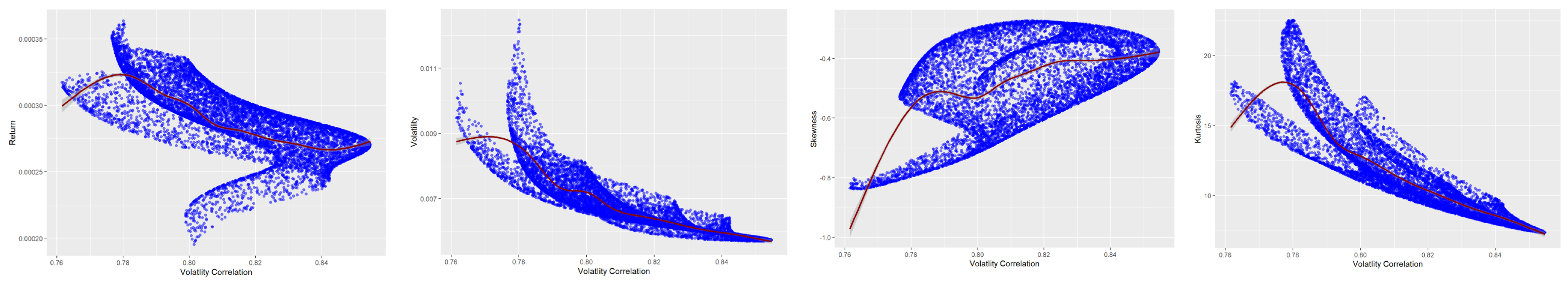
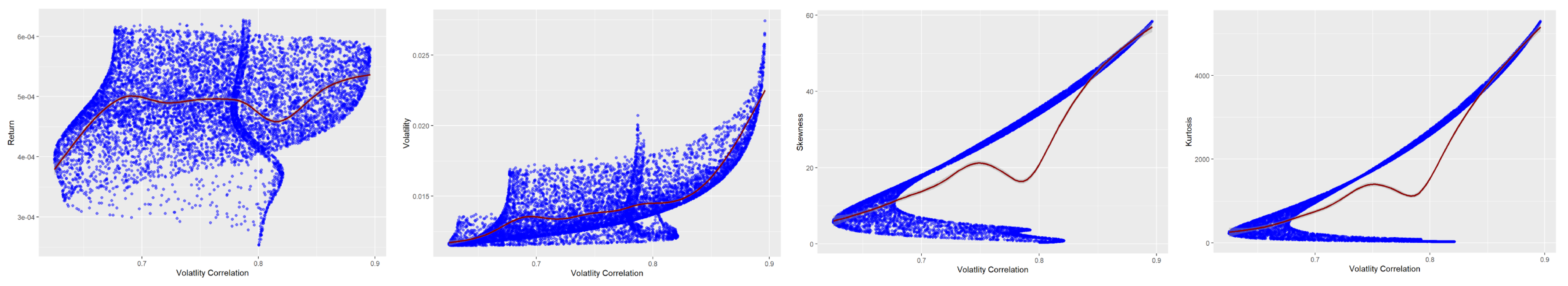
Figure 4, Figure 5 and Figure 6 visualize the relationship between portfolio return skewness and kurtosis using random weights. For stocks, the expected portfolio return increases as the portfolio skewness increases and kurtosis decreases. Thus, the expected portfolio return and PSR can be increased by minimizing portfolio kurtosis and maximizing portfolio skewness. Similar conclusions can be drawn for the first group of cryptocurrencies based on Figure 5. However, the second group of cryptocurrencies shows an insignificant correlation between portfolio return, skewness, and kurtosis (Figure 6). We further investigate the relationship between portfolio skewness and kurtosis as the volatility correlation increases, and Figure 7, Figure 8 and Figure 9 summarize the results. Increasing the volatility correlation can generally raise PSR and predicted portfolio return. However, the rate of increase is different for the three groups, and stocks are expected to have the highest expected increment in return and PSR with volatility correlation increase.
Optimal weights for the minimum risk (variance) portfolio using SD, VEV, VES, VESV, and MAD are given in Table 2 for three groups. The table also provides annualized portfolio return, risk, and PSR for each risk measure for all the assets. Note that considering the first group of cryptocurrencies the highest weights are assigned to BTC, ETH, and BNB, respectively, under all risk measures. For the second group of cryptocurrencies, the highest portion of the investment is assigned to XRP under all risk measures. Except for the MAD, DOGE accounts for the second-highest weight in the second group of cryptocurrencies. Among the stocks, under all risk measures, ADBE (Adobe) is assigned the lowest weight, and the second-highest weight is taken by MRVL (Marvel).
The study also investigates optimal weight assignments of assets under SD, VEV, VES, VESV, and MAD for tangency portfolio and maximum mean risk portfolio. Summarized results for tangency and maximum mean risk portfolio are given in Table 3. The optimal weight assignment for the first group of cryptocurrencies under the maximum mean risk portfolio is similar to that of the minimum variance portfolio. However, for the second group of cryptocurrencies, the optimal weight assignment varies among the risk measures. Among the stocks, AAPL has the highest optimal weight for all the risk measures. ADBE has the lowest optimal weights among the stocks for all the risk measures, following the same results as in the minimum variance portfolio.
Optimal weight assignments of minimum risk portfolio and maximum mean risk portfolio are visualized in Figure 10, Figure 11 and Figure 12 for three asset groups. Note that stocks with low risks, such as AMZN, AAPL, and MSFT, cryptocurrencies with low risks, such as BTC and XRP, are assigned more weights under the minimum risk portfolio under VESV. In contrast, stocks with high risk-adjusted for expected return such as AAPL and MRVL are assigned more weights under the maximum mean risk portfolio under VESV. It is important to note that BTC from cryptocurrency group 1 and XRP from cryptocurrency group 2 are assigned more weights under both minimum risk and maximum mean risk portfolios.
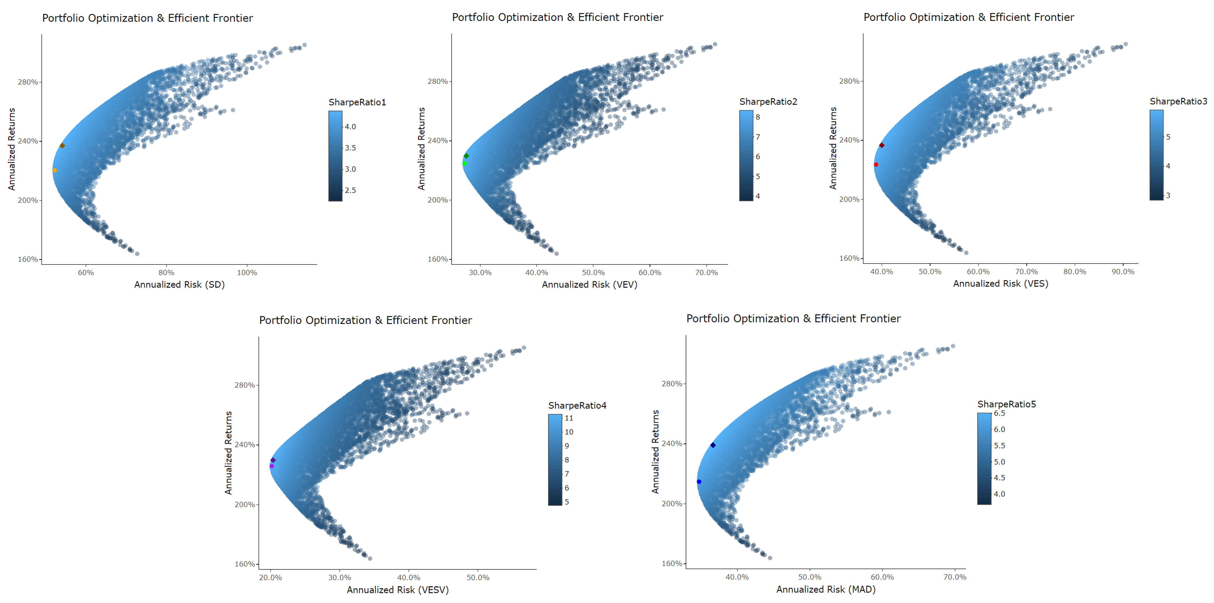
Figure 13, Figure 14 and Figure 15 provide the effective borders of three asset groups’ lowest risk and maximum mean risk portfolios utilizing SD, VEV, VES, VESV, and MAD. In addition, there is a greater APSR for each maximum mean-risk portfolio than for the matching minimal risk portfolio. Note that efficient frontiers for stocks are more scattered compared to cryptocurrency groups, and for cryptocurrencies, annualized returns are very high compared to that of stocks. However, cryptocurrencies also account for high annualized risk compared to stocks.
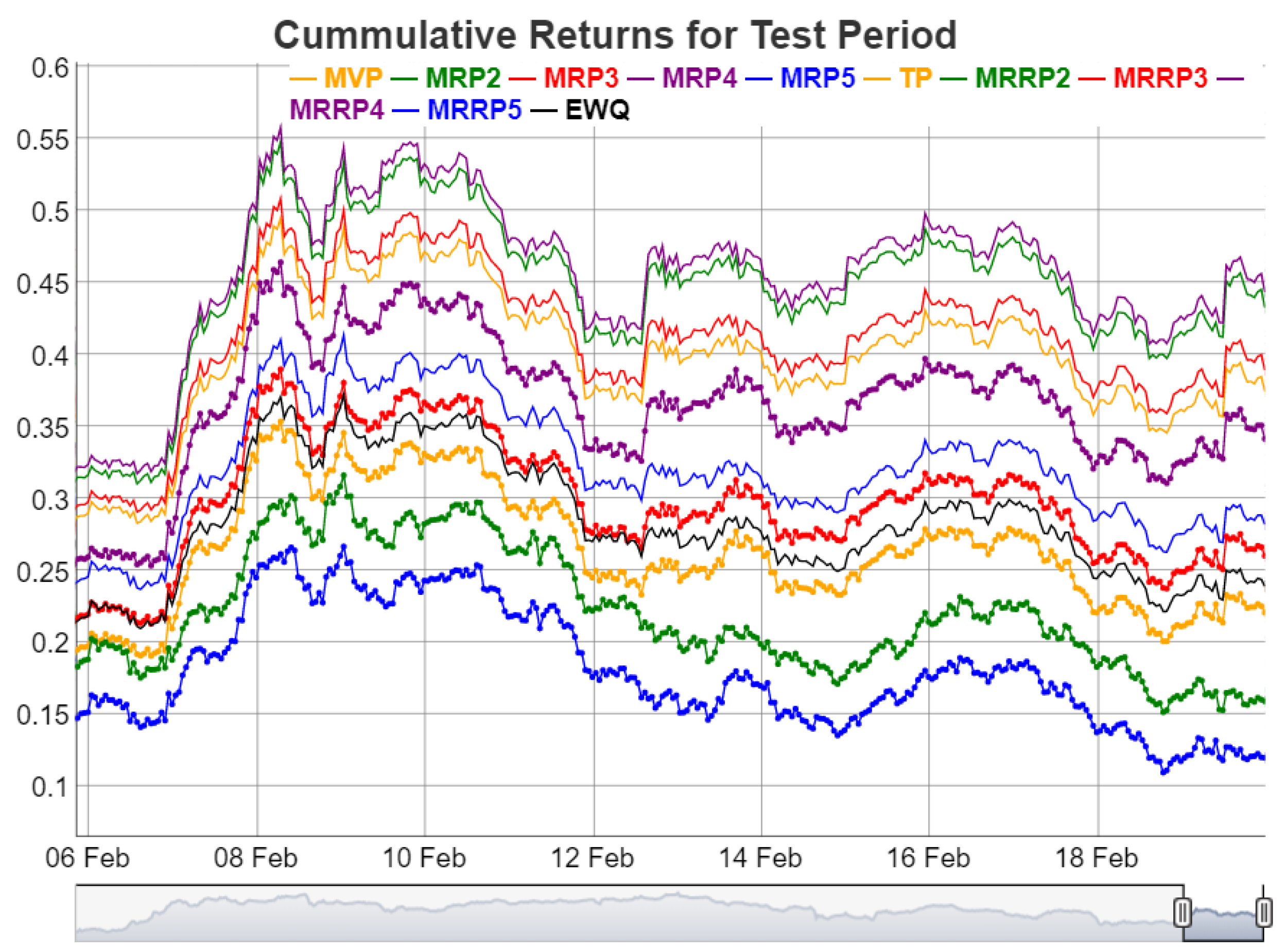
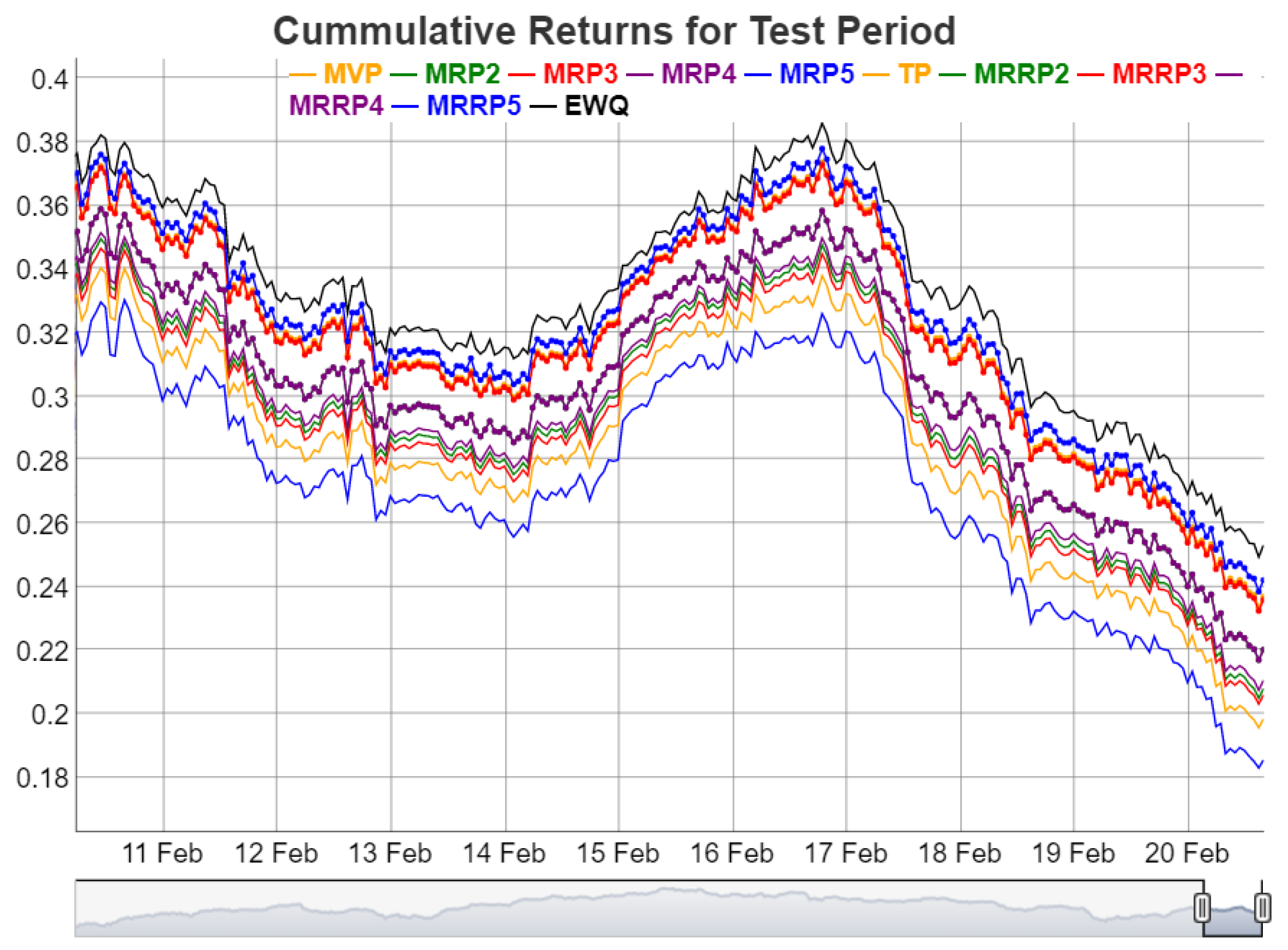
Considering the test data of three asset groups, Figure 16, Figure 17 and Figure 18 visualize cumulative returns of the portfolios. The black line represents cumulative returns of the portfolios with equal weights (EWQ). The cumulative returns of the minimum and maximum mean risk portfolio using SD, VEV, VES, VESV, and MAD are represented by bottom and top orange, green, red, and purple lines, respectively. Note that, in general, maximum mean risk portfolios perform better than minimum risk portfolios for stocks (Figure 16). However, the performance of minimum risk and maximum mean risk portfolios are very close (Figure 17 and Figure 18), and, still, maximum mean risk portfolios outperform minimum risk portfolios.
5. Conclusions
Cryptocurrencies face risks such as volatility, lack of regulation in their trade, hacker risk, etc., and the resulting portfolios constructed with cryptocurrencies are very risky. A straightforward yet powerful data-driven portfolio risk measure integrating skewness and kurtosis is provided to obtain optimal portfolio weights for cryptocurrency assets using the hourly price data. The novelty of the paper is to use the recently proposed volatility correlation-based portfolio risk measure and construct resilient portfolios for cryptocurrencies without inverting the higher order covariance matrix of the portfolio returns as used in many traditional approaches.
Our experimental observations suggest that hourly adjusted closing prices capture more detailed and comprehensive analysis, making a high-frequency analysis with big data possible. High-frequency data also reveal a very high excess kurtosis for returns of cryptocurrencies. Moreover, this study emphasizes the superiority of portfolio selection using data-driven methods over the traditional portfolio standard deviation methods.
It is important to point out that optimal weights are chosen from a pool of weights generated from a uniform distribution. Even though 8000 combinations of random weights are considered in the study, the ideal approach is to obtain optimal weights by solving an optimization problem. However, it requires high computation power, and it is to be believed beyond the scope of this study. Furthermore, the study does not investigate portfolios with a combination of financial instruments from three groups, as would be the case in many real-life situations. Future research will consider mixed portfolios of three groups with more stocks and cryptocurrencies, which is a natural extension of this work.
Author Contributions
Data curation, S.B. and J.S.; Formal analysis, S.B. and J.S.; Methodology, J.S.; Validation, S.B. and J.S.; Visualization, S.B. and J.S.; Writing—original draft, S.B. and J.S.; Writing—review & editing, S.B. and J.S. All authors have read and agreed to the published version of the manuscript.
Funding
This research received no external funding.
Data Availability Statement
Supporting data and codes of the study can be found in https://github.com/sulabola/Portfolio_Optimization2022.git, accessed on 18 August 2022.
Acknowledgments
The first author acknowledges the Graduate Entrance Scholarship in Statistics (GESS) and Faculty of Science Enhancement of Grant Stipends (SEGS), University of Manitoba. The second author acknowledges the Faculty of Graduate Enhancement of Tri-Agency Stipends (GETS), University of Manitoba.
Conflicts of Interest
The authors declare no conflict of interest.
Appendix A
The selection of cryptocurrencies is based on market capitalization, and Coinmarketcap (http://www.coinmarketcap.com, accessed on 18 August 2022) CoinMarketCap (n.d.) is a potential source of information on the market capitalization of each asset. Even though high-frequency data for cryptocurrencies are available in Yahoo! Finance (http://www.finance.yahoo.com, accessed on 18 August 2022) YahooFinance (n.d.) and most of the analysis is conducted using RStudio, RStudio fails to download high-frequency data directly from the source. However, Python is capable of downloading high-frequency data, and portfolio optimization is carried out using RStudio.
Download data using Python:
In order to Install “yfinance” type “pip install yfinance” on anaconda terminal.
          import pandas as pd
          import yfinance as yf
          stock = "BTC-USD"
          start_date = "2018-05-01"
          df_btc_daily = yf.download(stock,
          start = start_date, interval= "1h").reset_index()
          df_btc_daily.to_csv(’./HourlyData.csv’,
          index = False)
Three sets of R codes are required for the three asset groups considered in the study. The required data are saved in the Excel files (e.g., for Bitcoin). If data files and R codes are in the same folder, it is not necessary to set up paths of data files manually in RStudio.References
- Aljinović, Zdravka, Branka Marasović, and Tea Šestanović. 2021. Cryptocurrency Portfolio Selection—A Multicriteria Approach. Mathematics 9: 1677. [Google Scholar] [CrossRef]
- Appel, Dominik, and Michael Grabinski. 2011. The origin of financial crisis: A wrong definition of value. Portuguese Journal of Quantitative Methods 2: 33–51. [Google Scholar]
- Basilio, Marcio Pereira, Jessica Galdino de Freitas, Milton George Fonseca Kämpffe, and Ricardo Bordeaux Rego. 2018. Investment portfolio formation via multicriteria decision aid: A Brazilian stock market study. Journal of Modelling in Management 23: 394–417. [Google Scholar] [CrossRef]
- Baur, Dirk G., and Thomas Dimpfl. 2018. Asymmetric volatility in cryptocurrencies. Economics Letters 173: 148–51. [Google Scholar] [CrossRef]
- Best, Michael J. 2010. Portfolio Optimization. Boca Raton: CRC Press. [Google Scholar]
- Cryptocurrency Prices, Charts and Market Capitalizations|CoinMarketCap. n.d. Available online: https://coinmarketcap.com/ (accessed on 18 August 2022).
- Grabinski, Michael, and Galiya Klinkova. 2020. Scrutinizing Distributions Proves That IQ Is Inherited and Explains the Fat Tail. Applied Mathematics 11: 957. [Google Scholar] [CrossRef]
- Juškaitė, Lina, and Laura Gudelytė-Žilinskienė. 2022. Investigation of the feasibility of including different cryptocurrencies in the investment portfolio for its diversification. Business, Management and Economics Engineering 20: 172–88. [Google Scholar] [CrossRef]
- Klinkova, Galiya, and Michael Grabinski. 2017. Due to Instability Gambling is the best Model for most Financial Products. Archives of Business Research 5: 255–61. [Google Scholar] [CrossRef]
- Lai, Kin Keung, Lean Yu, and Shouyang Wang. 2006. Mean-variance-skewness-kurtosis-based portfolio optimization. Papers presented at First International Multi-Symposiums on Computer and Computational Sciences (IMSCCS’06), Hangzhou, China, June 20–24; vol. 2, pp. 292–97. [Google Scholar]
- Liang, You, Aera Thavaneswaran, and Bovas Abraham. 2011. Joint estimation using quadratic estimating function. Journal of Probability and Statistics 2011: 372512. [Google Scholar] [CrossRef]
- Liang, You, Aerambamoorthy Thavaneswaran, Zimo Zhu, Ruppa K. Thulasiram, and Md Erfanul Hoque. 2020. Data-Driven Adaptive Regularized Risk Forecasting. Papers presented at 2020 IEEE 44th Annual Computers, Software, and Applications Conference (COMPSAC), Madrid, Spain, July 13–17; pp. 1296–301. [Google Scholar]
- Ma, Yechi, Ferhana Ahmad, Miao Liu, and Zilong Wang. 2020. Portfolio optimization in the era of digital financialization using cryptocurrencies. Technological Forecasting and Social Change 161: 120265. [Google Scholar] [CrossRef] [PubMed]
- Nakamoto, Satoshi. 2008. Bitcoin: A peer-to-peer electronic cash system. Decentralized Business Review 2008: 21260. [Google Scholar]
- Pätäri, Eero, Timo Leivo, and Samuli Honkapuro. 2012. Enhancement of equity portfolio performance using data envelopment analysis. European Journal of Operational Research 220: 786–97. [Google Scholar] [CrossRef]
- Peng, Yaohao, Pedro Henrique Melo Albuquerque, Jader Martins Camboim de Sá, Ana Julia Akaishi Padula, and Mariana Rosa Montenegro. 2018. The best of two worlds: Forecasting high frequency volatility for cryptocurrencies and traditional currencies with Support Vector Regression. Expert Systems with Applications 97: 177–92. [Google Scholar] [CrossRef]
- Selection, Portfolio. 1959. Efficient Diversification of Investments. New York: John Wiley & Sons. [Google Scholar]
- Thompson, M. E., and A. Thavaneswaran. 1999. Filtering via estimating functions. Applied Mathematics Letters 12: 61–67. [Google Scholar] [CrossRef]
- Thavaneswaran, Aerambamoorthy, Ruppa K. Thulasiram, Zimo Zhu, Mohammed Erfanul Hoque, and Nalini Ravishanker. 2019. Fuzzy Value-at-Risk forecasts using a novel data-driven neuro volatility predictive model. Papers presented at 2019 IEEE 43rd Annual Computer Software and Applications Conference (COMPSAC), Milwaukee, WI, USA, July 15–19; vol. 2, pp. 221–26. [Google Scholar]
- Thavaneswaran, Aerambamoorthy, Alex Paseka, and Julieta Frank. 2020. Generalized value at risk forecasting. Communications in Statistics—Theory and Methods 49: 4988–95. [Google Scholar] [CrossRef]
- Thavaneswaran, Aerambamoorthy, You Liang, Na Yu, Alex Paseka, and Ruppa K. Thulasiram. 2021. Novel Data-Driven Resilient Portfolio Risk Measures Using Sign and Volatility Correlations. Papers presented at 2021 IEEE 45th Annual Computers, Software, and Applications Conference (COMPSAC), Madrid, Spain, July 12–16; pp. 1742–47. [Google Scholar]
- The Bank for International Settlements. 2021. Basel III Monitoring Report. Bank for International Settlements. Available online: https://www.bis.org/bcbs/publ/d524.pdf (accessed on 10 March 2022).
- Yahoo Finance-Stock Market Live, Quotes, Business & Finance News. n.d. Available online: https://finance.yahoo.com/ (accessed on 18 August 2022).
- Zhu, Zimo, Aerambamoorthy Thavaneswaran, Alexander Paseka, Julieta Frank, and Ruppa Thulasiram. 2020. Portfolio optimization using a novel data-driven EWMA covariance model with big data. Papers presented at 2020 IEEE 44th Annual Computers, Software, and Applications Conference (COMPSAC), Madrid, Spain, July 13–17; pp. 1308–13. [Google Scholar]
Figure 1.
Hourly adjusted closing prices of stocks.
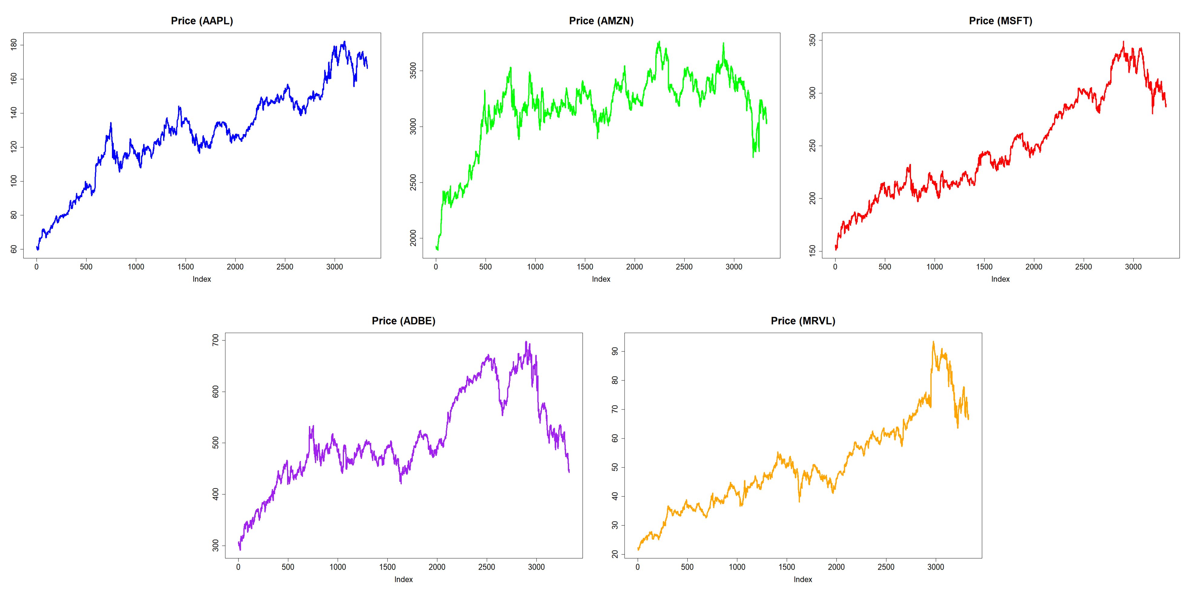
Figure 2.
Hourly adjusted closing prices of cryptocurrencies (Group 1).
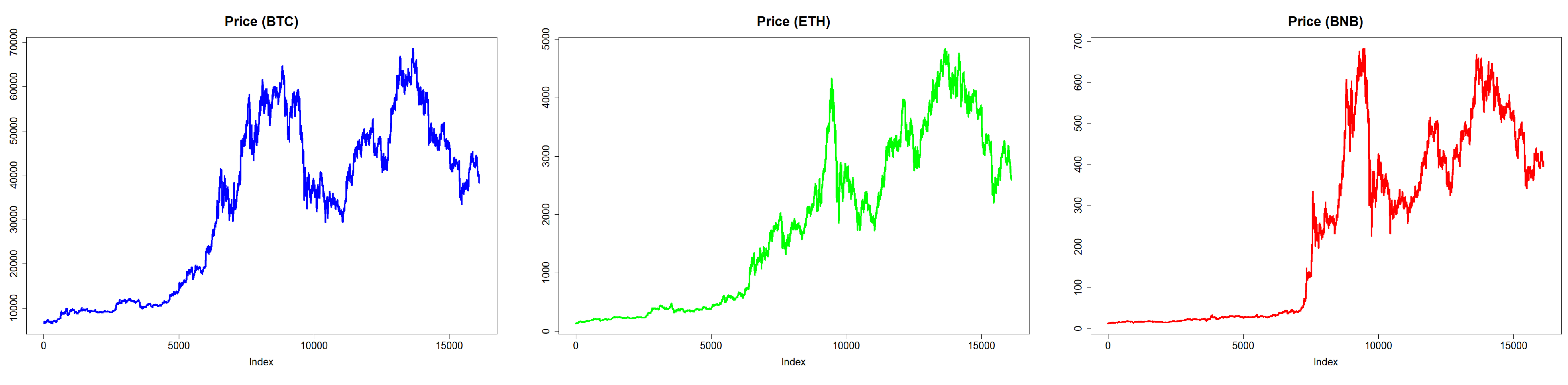
Figure 3.
Hourly adjusted closing prices of cryptocurrencies (Group 2).
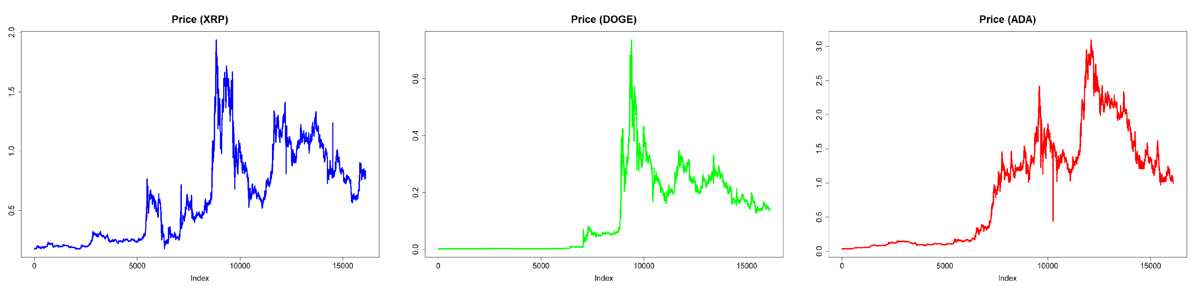
Figure 4.
Scatterplot demonstrating the relationship between portfolio return, skewness, and kurtosis of Stocks.
Figure 4.
Scatterplot demonstrating the relationship between portfolio return, skewness, and kurtosis of Stocks.
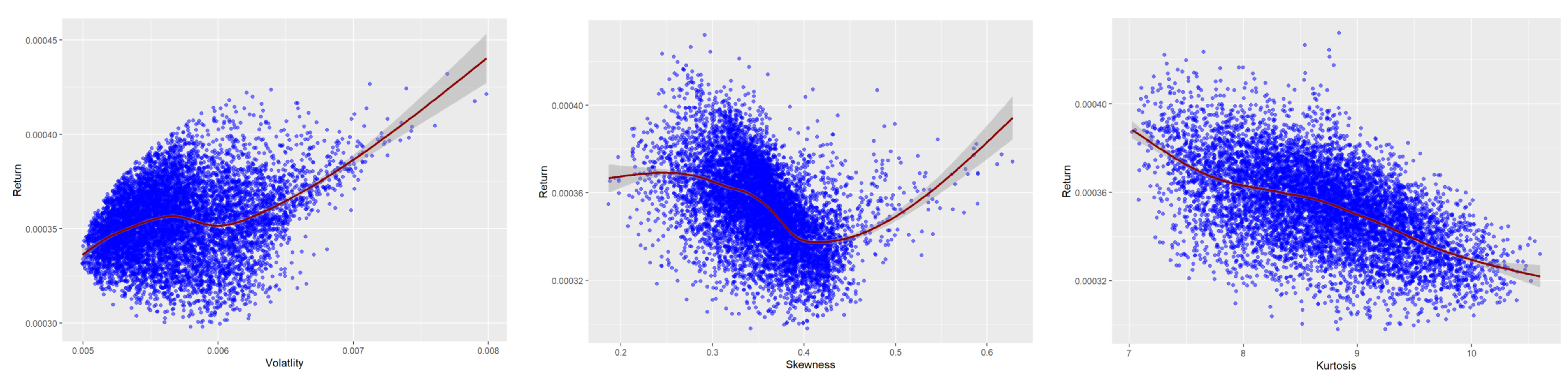
Figure 5.
Scatterplot demonstrating relationship between portfolio return, skewness, and kurtosis of Cryptocurrencies (Group 1).
Figure 5.
Scatterplot demonstrating relationship between portfolio return, skewness, and kurtosis of Cryptocurrencies (Group 1).
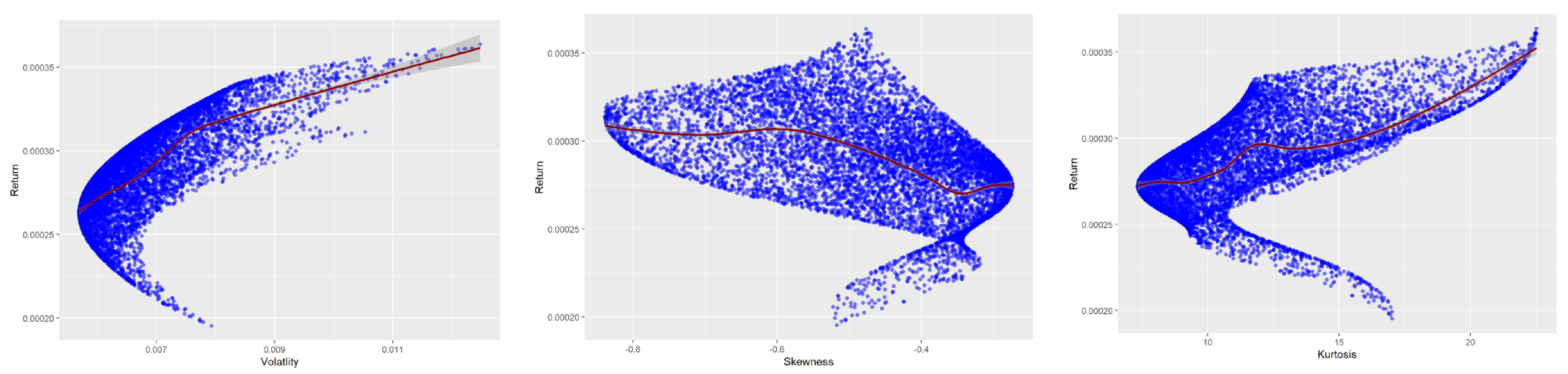
Figure 6.
Scatterplot demonstrating relationship between portfolio return, skewness, and kurtosis of Cryptocurrencies (Group 2).
Figure 6.
Scatterplot demonstrating relationship between portfolio return, skewness, and kurtosis of Cryptocurrencies (Group 2).
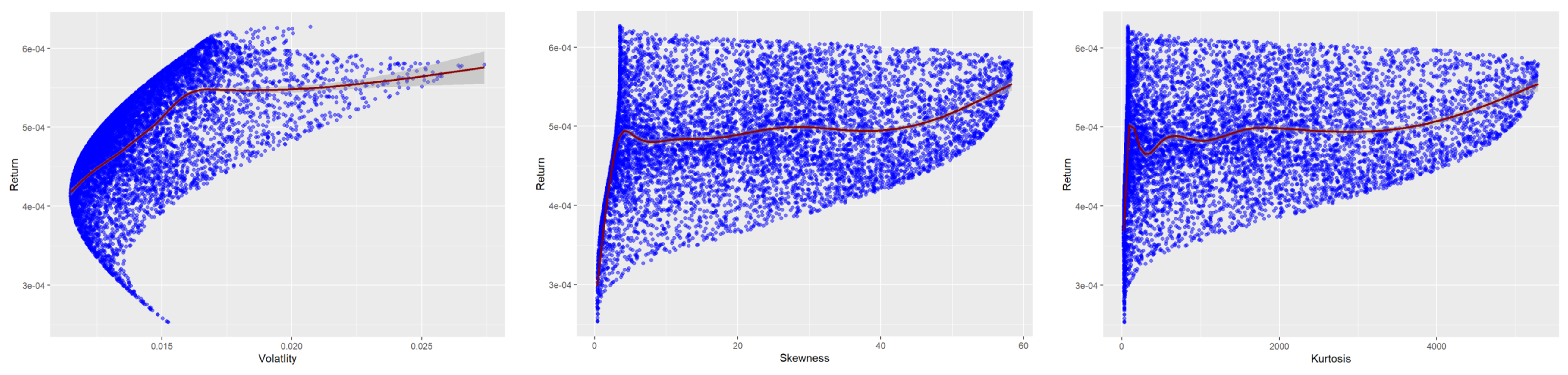
Figure 7.
Relationship between mean, volatility, skewness, kurtosis, and volatility correlation of Stocks.
Figure 7.
Relationship between mean, volatility, skewness, kurtosis, and volatility correlation of Stocks.

Figure 8.
Relationship between mean, volatility, skewness, kurtosis, and volatility correlation of Cryptocurrencies (Group 1).
Figure 8.
Relationship between mean, volatility, skewness, kurtosis, and volatility correlation of Cryptocurrencies (Group 1).

Figure 9.
Relationship between mean, volatility, skewness, kurtosis, and volatility correlation of Cryptocurrencies (Group 2).
Figure 9.
Relationship between mean, volatility, skewness, kurtosis, and volatility correlation of Cryptocurrencies (Group 2).

Figure 10.
The asset weights assigned using MRP-VESV and MMRP-VESV for Stock Assets.
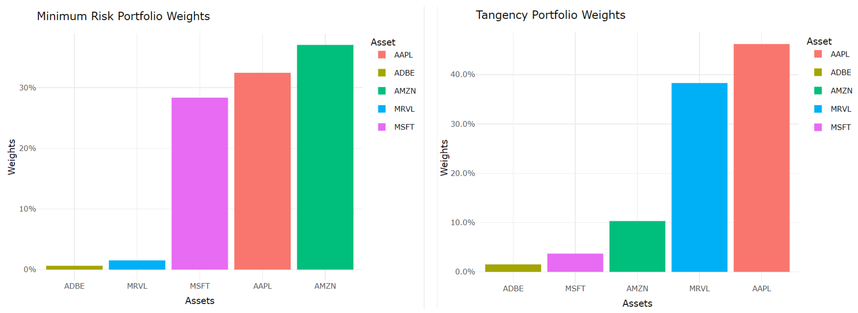
Figure 11.
The asset weights assigned using MRP-VESV and MMRP-VESV for Cryptocurrency (Group 1) assets.
Figure 11.
The asset weights assigned using MRP-VESV and MMRP-VESV for Cryptocurrency (Group 1) assets.
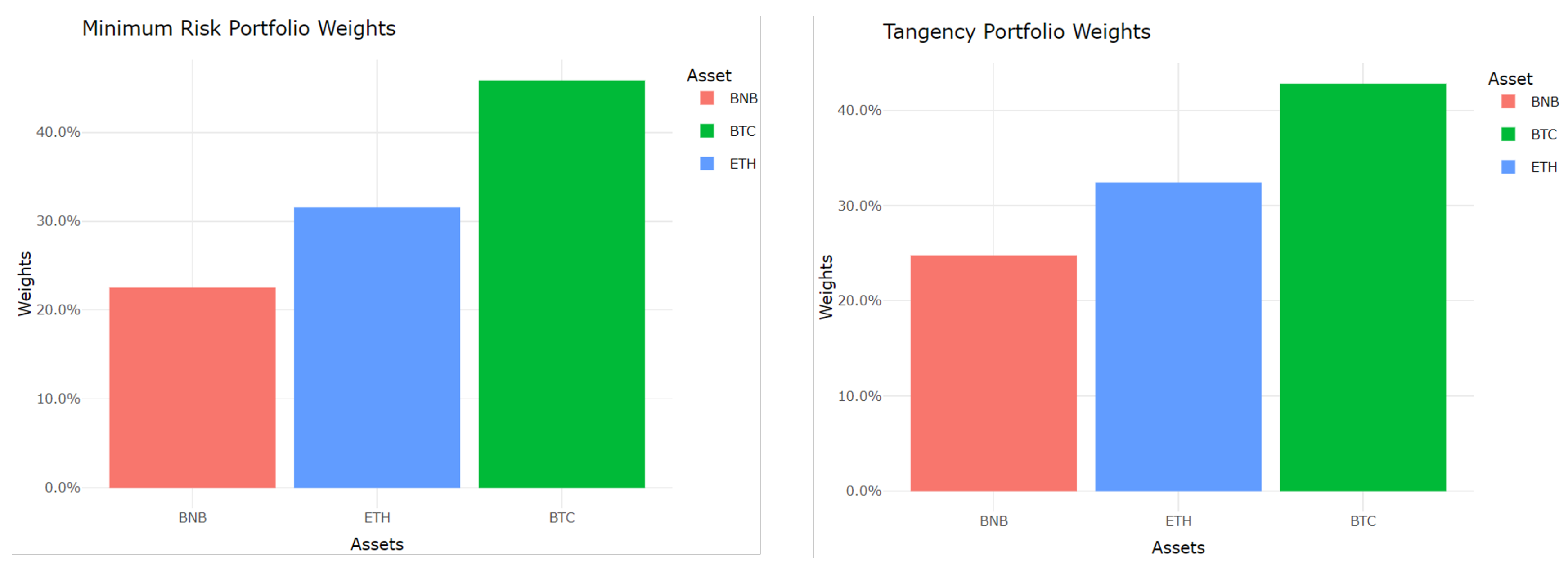
Figure 12.
The asset weights assigned using MRP-VESV and MMRP-VESV for Cryptocurrency (Group 2) assets.
Figure 12.
The asset weights assigned using MRP-VESV and MMRP-VESV for Cryptocurrency (Group 2) assets.
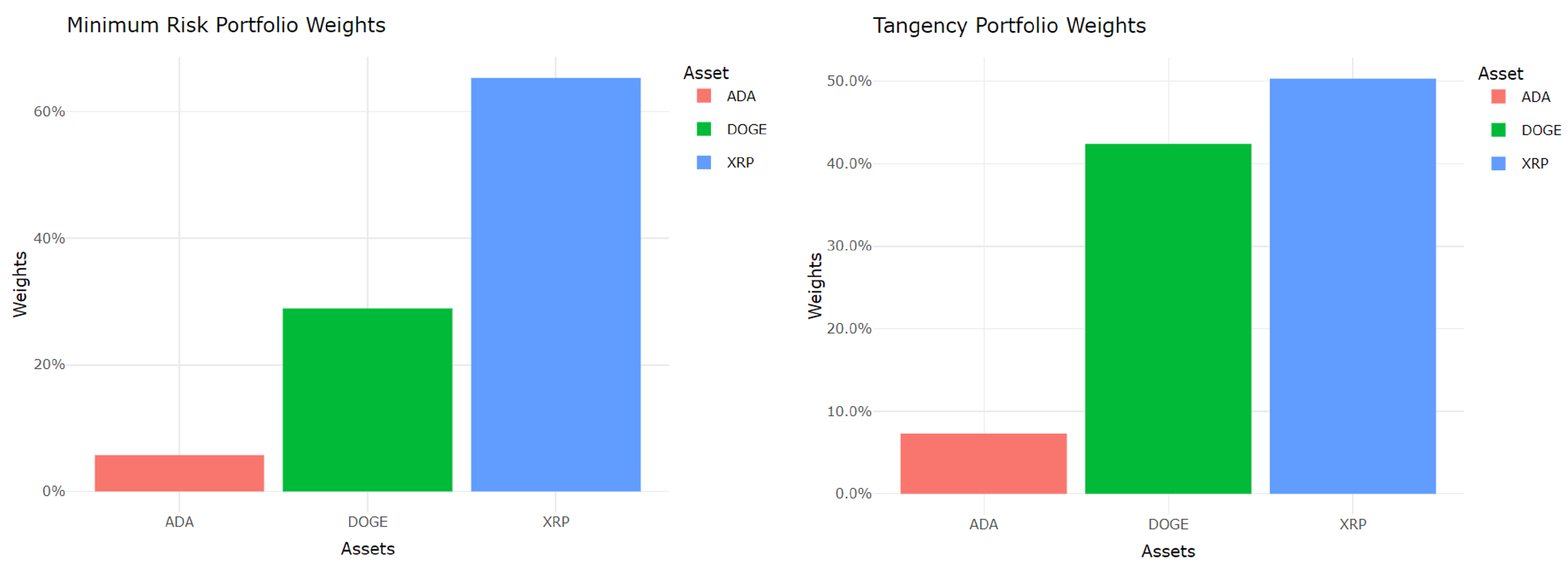
Figure 13.
Efficient frontiers of Stocks.
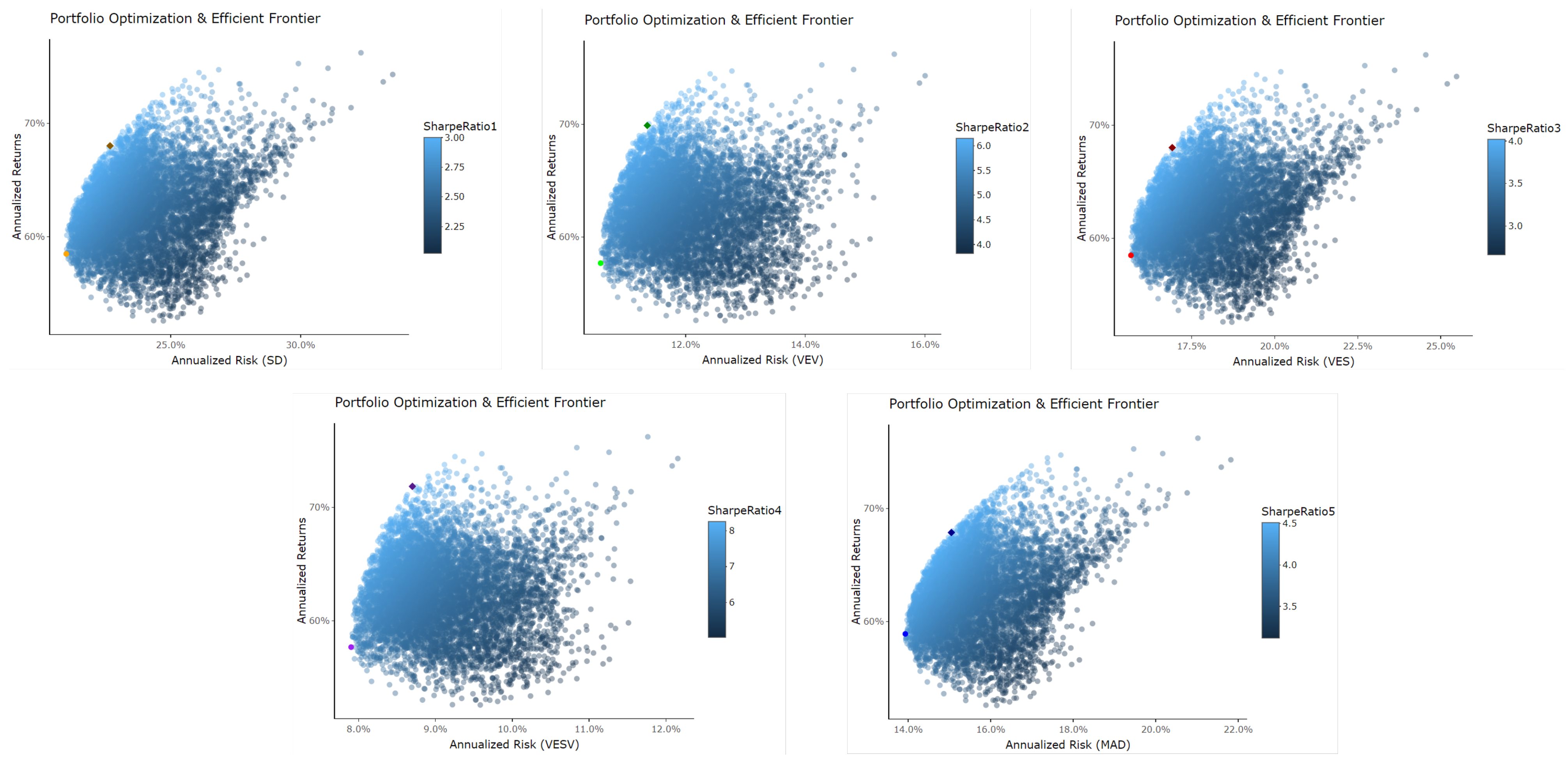
Figure 14.
Efficient frontiers of Cryptocurrencies (Group 1).

Figure 15.
Efficient frontiers of Cryptocurrencies (Group 2).
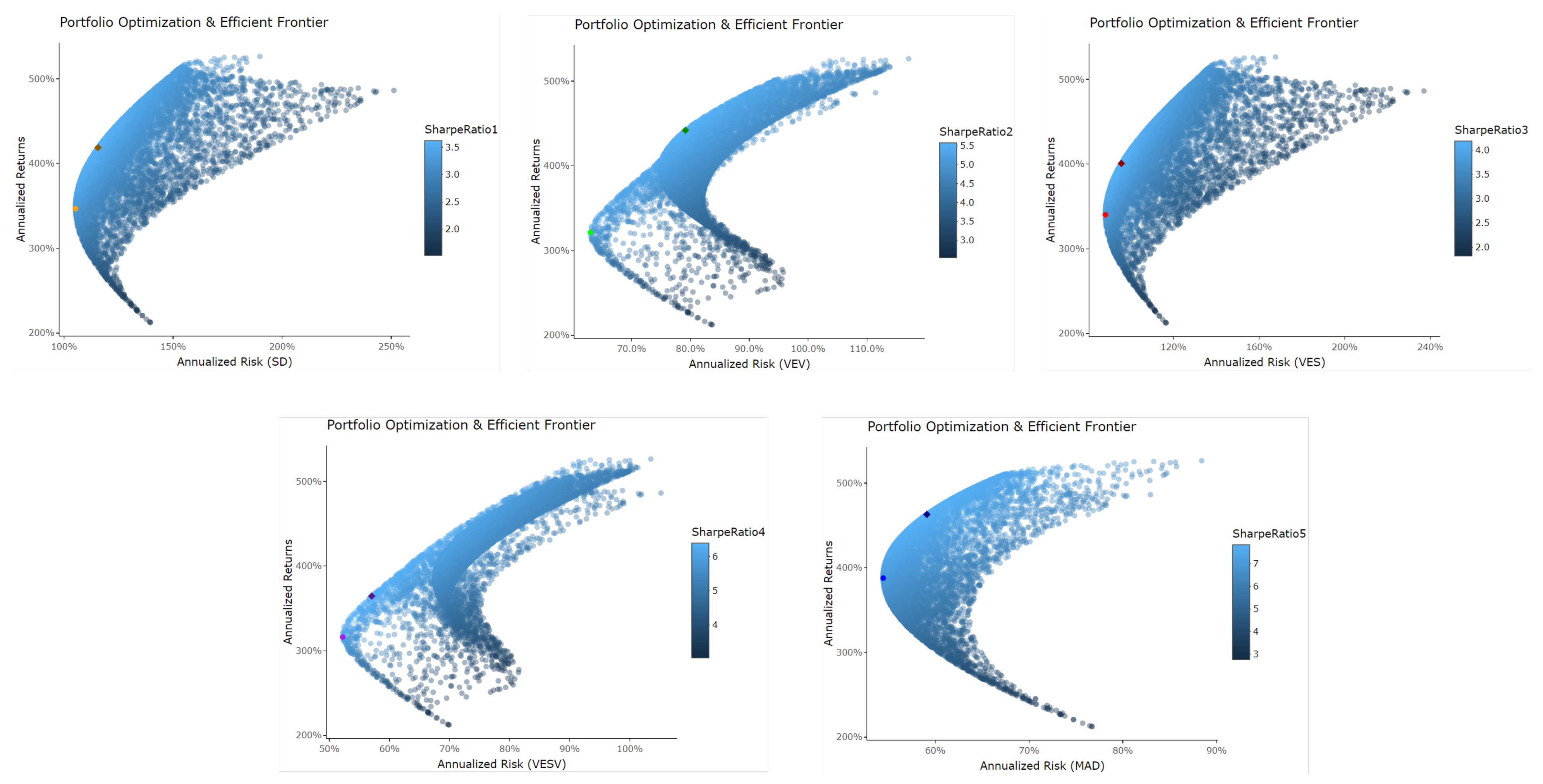
Figure 16.
Cumulative returns of Stocks.
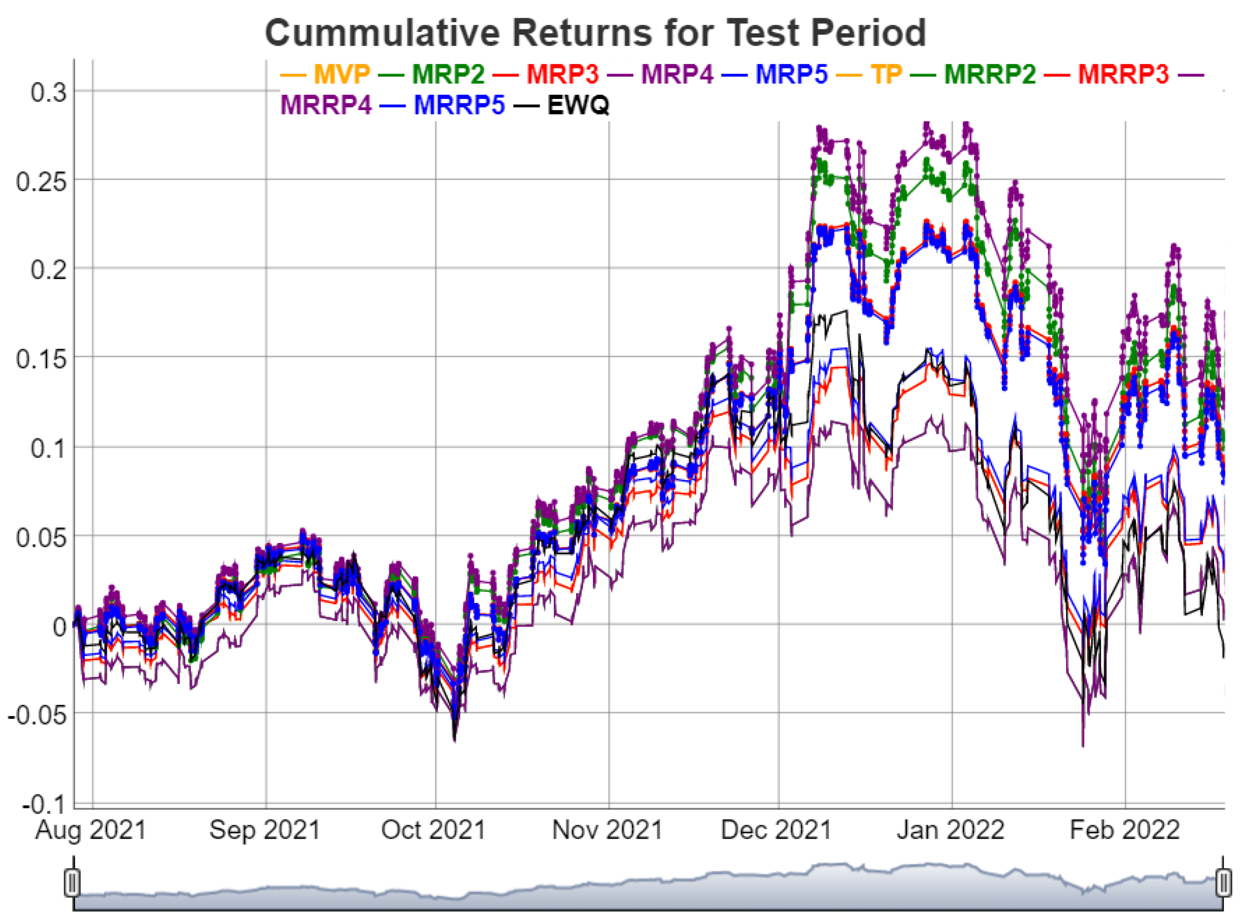
Figure 17.
Cumulative returns of Cryptocurrencies (Group 1).

Figure 18.
Cumulative returns of Cryptocurrencies (Group 2).

Table 1.
Summary statistics of returns of Stocks and Cryptocurrencies.
| Asset | SD | |||||
|---|---|---|---|---|---|---|
| AAPL | 0.0004 | 0.0074 | 0.8731 | 0.6415 | 0.6441 | 9.8464 |
| AMZN | 0.0003 | 0.0070 | 0.8661 | 0.6403 | 0.3468 | 10.0728 |
| MSFT | 0.0003 | 0.0063 | 0.8771 | 0.6501 | 0.4758 | 8.4047 |
| ADBE | 0.0003 | 0.0076 | 0.8459 | 0.6470 | 0.4501 | 10.7409 |
| MRVL | 0.0005 | 0.0097 | 0.8692 | 0.6504 | 0.2968 | 9.7388 |
| BTC | 0.0002 | 0.0081 | 0.8017 | 0.6119 | −0.5150 | 17.0001 |
| ETH | 0.0003 | 0.0106 | 0.7626 | 0.6309 | −0.8026 | 18.1163 |
| BNB | 0.0004 | 0.0127 | 0.7802 | 0.6103 | −0.4764 | 22.5072 |
| XRP | 0.0002 | 0.0156 | 0.8002 | 0.5494 | 0.3959 | 30.0385 |
| DOGE | 0.0006 | 0.0212 | 0.7871 | 0.4672 | 3.5403 | 76.9270 |
| ADA | 0.0006 | 0.0275 | 0.8962 | 0.3307 | 58.3452 | 5293.0679 |
: volatility correlation of the data sample, : sign correlation of the data sample. : sample skewness of the returns, : sample excess kurtosis of the returns.
Table 2.
Minimum risk portfolios of Stocks and Cryptocurrencies.
| MVP | MRP-VEV | MRP-VES | MRP-VESV | MRP-MAD | |
|---|---|---|---|---|---|
| AAPL | 0.3702 | 0.3245 | 0.3702 | 0.3245 | 0.3533 |
| AMZN | 0.2465 | 0.3705 | 0.2465 | 0.3705 | 0.2162 |
| MSFT | 0.3507 | 0.2835 | 0.3508 | 0.2835 | 0.3615 |
| ADBE | 0.0119 | 0.0063 | 0.0119 | 0.0063 | 0.0266 |
| MRVL | 0.0207 | 0.0152 | 0.0207 | 0.0152 | 0.0424 |
| Return | 0.5847 | 0.5767 | 0.5847 | 0.5767 | 0.5889 |
| Risk | 0.2098 | 0.1058 | 0.1568 | 0.0790 | 0.1393 |
| APSR | 2.7869 | 5.4501 | 3.7305 | 7.2956 | 4.2276 |
| BTC | 0.5050 | 0.4666 | 0.4796 | 0.4587 | 0.5492 |
| ETH | 0.2887 | 0.3139 | 0.2984 | 0.3157 | 0.2703 |
| BNB | 0.2063 | 0.2195 | 0.2222 | 0.2256 | 0.1804 |
| Return | 2.2027 | 2.2470 | 2.2354 | 2.2576 | 2.1470 |
| Risk | 0.5223 | 0.2723 | 0.3882 | 0.2018 | 0.3478 |
| APSR | 4.2175 | 8.2529 | 5.7586 | 11.1857 | 6.1724 |
| XRP | 0.5442 | 0.6379 | 0.5671 | 0.6532 | 0.3967 |
| DOGE | 0.2889 | 0.3085 | 0.2841 | 0.2891 | 0.2752 |
| ADA | 0.1669 | 0.0536 | 0.1488 | 0.0577 | 0.3281 |
| Return | 3.4690 | 3.2140 | 3.4024 | 3.1624 | 3.8780 |
| Risk | 1.0528 | 0.6303 | 0.8827 | 0.5222 | 0.5444 |
| ASPR | 3.2950 | 5.0992 | 3.8546 | 6.0556 | 7.1231 |
MVP: Minimum Variance Portfolio using SD; MRP-VEV: Minimum Risk Portfolio using VEV.
Table 3.
Maximum mean-risk portfolios of Stocks and Cryptocurrencies.
| TP | MMRP-VEV | MMRP-VES | MMRP-VESV | MMRP-MAD | |
|---|---|---|---|---|---|
| AAPL | 0.4774 | 0.3802 | 0.4774 | 0.4619 | 0.4563 |
| AMZN | 0.1462 | 0.1648 | 0.1462 | 0.1030 | 0.1572 |
| MSFT | 0.0833 | 0.0743 | 0.0833 | 0.0370 | 0.0838 |
| ADBE | 0.0489 | 0.0115 | 0.0489 | 0.0152 | 0.0518 |
| MRVL | 0.2442 | 0.3692 | 0.2442 | 0.3829 | 0.2509 |
| Return | 0.6801 | 0.6989 | 0.6801 | 0.7184 | 0.6786 |
| Risk | 0.2267 | 0.1136 | 0.1692 | 0.0870 | 0.1505 |
| APSR | 3.0004 | 6.1519 | 4.0201 | 8.2566 | 4.5101 |
| BTC | 0.3719 | 0.4280 | 0.3742 | 0.4280 | 0.3574 |
| ETH | 0.3451 | 0.3243 | 0.3461 | 0.3243 | 0.3459 |
| BNB | 0.2830 | 0.2477 | 0.2797 | 0.2477 | 0.2967 |
| Return | 2.3701 | 2.2982 | 2.3662 | 2.2982 | 2.3907 |
| Risk | 0.5415 | 0.2754 | 0.4001 | 0.2038 | 0.3671 |
| APSR | 4.3773 | 8.3449 | 5.9134 | 11.2767 | 6.5131 |
| XRP | 0.3137 | 0.1996 | 0.3742 | 0.5030 | 0.1513 |
| DOGE | 0.4457 | 0.2446 | 0.4214 | 0.4239 | 0.4117 |
| ADA | 0.2407 | 0.5558 | 0.2044 | 0.0732 | 0.4370 |
| Return | 4.1881 | 4.4193 | 4.0069 | 3.6453 | 4.6300 |
| Risk | 1.1561 | 0.7917 | 0.9568 | 0.5705 | 0.5910 |
| APSR | 3.6226 | 5.5822 | 4.1877 | 6.3897 | 7.8347 |
TP: Tangency Portfolio using SD; MMRP-VEV: Maximum Mean Risk Portfolio using VEV.
Publisher’s Note: MDPI stays neutral with regard to jurisdictional claims in published maps and institutional affiliations. |
© 2022 by the authors. Licensee MDPI, Basel, Switzerland. This article is an open access article distributed under the terms and conditions of the Creative Commons Attribution (CC BY) license (https://creativecommons.org/licenses/by/4.0/).
Share and Cite
MDPI and ACS Style
Bowala, S.; Singh, J. Optimizing Portfolio Risk of Cryptocurrencies Using Data-Driven Risk Measures. J. Risk Financial Manag. 2022, 15, 427. https://doi.org/10.3390/jrfm15100427
AMA Style
Bowala S, Singh J. Optimizing Portfolio Risk of Cryptocurrencies Using Data-Driven Risk Measures. Journal of Risk and Financial Management. 2022; 15(10):427. https://doi.org/10.3390/jrfm15100427
Chicago/Turabian StyleBowala, Sulalitha, and Japjeet Singh. 2022. "Optimizing Portfolio Risk of Cryptocurrencies Using Data-Driven Risk Measures" Journal of Risk and Financial Management 15, no. 10: 427. https://doi.org/10.3390/jrfm15100427