Abstract
Seabed sedimentary bedforms (SSBs) are strong indicators of current flow (direction and velocity) and can be mapped in high resolution using multibeam echosounders. Many approaches have been designed to automate the classification of such SSBs imaged in multibeam echosounder data. However, these classification systems only apply a geomorphological contextualisation to the data without making direct assertions on the velocities of benthic currents that form these SSBs. Here, we apply an object-based image analysis (OBIA) workflow to derive a geomorphological classification of SSBs in the Moira Mounds area of the Belgica Mound Province, NE Atlantic through k-means clustering. Cold-water coral reefs as sessile filter-feeders benefit from strong currents are often found in close association with sediment wave fields. This OBIA provided the framework to derive SSB wavelength and wave height, these SSB attributes were used as predictor variables for a multiple linear regression to estimate current velocities. Results show a bimodal distribution of current flow directions and current speed. Furthermore, a 5 k-means classification of the SSB geomorphology exhibited an imprinting of current flow consistency which altered throughout the study site due to the interaction of regional, local, and micro scale topographic steering forces. This study is proof-of-concept for an assessment tool applied to vulnerable marine ecosystems but has wider applications for applied seabed appraisals and can inform management and monitoring practice across a variety of spatial and temporal scales. Deriving spatial patterns of hydrodynamic processes from widely available multibeam echosounder maps is pertinent to many avenues of research including scour predictions for offshore structures such as wind turbines, sediment transport modelling, benthic fisheries, e.g., scallops, cable route and pipeline risk assessment and habitat mapping.
1. Introduction
Understanding the current regime affecting seabed environments and habitats therein is a recurrent research requirement. Not only are currents an important influence on habitat for various organisms, especially filter feeds, but current also have a direct control on seabed sediment grain-size and composition through selective sedimentation processes. In areas where current controlled sediment transport produces mobile bedforms such as sediment waves, these may offer a hazard to cables and pipelines which may become excavated and exposed [1]. Likewise, structures may also become buried over time. Interpreting benthic current speeds from bedform morphologies also enables appropriate infrastructure design and assists sediment transport modelling important for coastal erosion management or to predict recovery from marine aggregate extraction [2,3,4]. Cold-water corals (CWCs) are sessile organisms that can generate complex three-dimensional frameworks that form reefs and coral mounds over time by the accumulation of biological remains including coral rubble and the trapping of sediments [5,6]. Over hundreds of thousands to millions of years, such reefs may eventually form giant carbonate mounds through successive periods of growth [7,8]. Habitats constructed by framework building scleractinian CWCs support other marine species, including commercial fish species, and provide refuge, feeding grounds, and nurseries creating biodiversity hotspots [9,10,11,12]. Seabed sedimentary bedforms (SSBs) have been observed in many CWC habitats implicating an inherent connection between CWCs and strong benthic currents [5,13,14,15]. Moreover, studies developing palaeo-environmental reconstructions of CWC habitat conditions indicate that periods of CWC habitat decline have been linked to weakened current regimes [16,17]. This is not surprising as CWCs are filter feeders ensnaring and consuming suspended food particles thus, enhanced current speeds can increase the encounter rate of these suspended food particles with coral feeding apparatus [18,19]. Although the significance of CWC habitats to marine biodiversity has widely been acknowledged, anthropogenic activities and environmental changes in the deep sea continue to adversely impact these environments [20,21]. Furthermore, the slow recuperation rates for these habitats from such impacts underlines the need to elucidate the processes that govern the success of these vulnerable marine ecosystems and proactively assign protective status [22]. Effective conservation and management of these vulnerable marine ecosystems requires detailed and accurate spatial information to be acquired of CWC and their surrounding environment [23,24]. Providing an accurate portrayal of seabed environmental conditions requires the production of seabed habitat maps that are applicable at multiple scales [25,26].
Multibeam echosounder (MBES) data provides bathymetry and backscatter data that readily portrays the geomorphological context of the seafloor [27,28] offering an efficient input for seabed habitat maps, depicting the spatial distribution of CWCs and their relationship with the adjacent seabed environment [14,29,30]. Despite the availability of this technology, only 18% of the world’s oceans are mapped at a resolution akin to terrestrial datasets [31]. Consequently, several national and international initiatives have been established to ameliorate this data deficit [31,32,33]. Executing this goal necessitates the acquisition of significant volumes of data, which require processing to create seabed habitat maps [34]. Additionally, these seabed habitat maps need to be objective and replicable to ensure the consistency of the analysis when appraising these conditions over repeated surveys [35]. Manually interpreting such volumes of data is laborious, dependent on the expertise of the analyst, vulnerable to bias, and introduces variability to the production of seabed habitat maps [36,37,38]. Several approaches have been developed to automate the production of seabed habitat maps in CWC environments [21,24,26]. Object-based image analysis (OBIA) offers the ability to characterise groups of pixels into distinct image objects that relate directly to physical seabed features [39,40]. Spectral features acquired from SSBs enable frequency analysis to be incorporated into OBIA workflows [41]. Stow et al. [42] generated a bedform velocity matrix to offer estimations of current speed, current direction, and variability using similar spectral characteristics derived from the seafloor geomorphology. Moreover, this technique has been applied and proven effective in obtaining current speeds in CWC environments [14]. Despite the demonstrated advantages of spectral features as part of an OBIA workflow and the importance of hydrodynamic regimes to CWCs, these features have yet to be exploited to provide automated appraisals of current speed.
Here, we provide a semi-automated OBIA workflow designed to categorise CWC mounds and SSBs present within MBES bathymetric data using a geomorphological classification that depicts the consistency of the hydrodynamic regime and provides the framework for current velocity estimations A fast Fourier transform (FFT) was applied to bathymetric profiles derived from image objects associated with SSBs crests. Wavelength and wave height were calculated as part of this analysis and a current velocity estimate was obtained using a multiple linear regression generated from parameters outlined in Stow et al. [42]. Geomorphological characterisation of the SSB crest image objects was achieved using a k-means classification deployed on the morphological attributes associated with the crests including wavelength and wave height. This is the first study to provide a semi-automated OBIA characterisation of seabed hydrodynamics solely using MBES bathymetry. As expressed above, this has rich application but is applied here to better understand current speed controls on cold-water coral reefs.
Study Site
The Belgica Mound Province (BMP) is found at the eastern flank of a north–south trending embayment occurring along the Irish continental margin called the Porcupine Seabight in the NE Atlantic [43,44,45]. The BMP consists of two chains of CWC giant carbonate mounds orientated north–south occurring at 650 m depth and 950 m, respectively [45,46,47]. A portion of the BMP is encompassed by a Special Area of Conservation (SAC) designated under the EU habitats Directive [48]. The BMP hosts several examples of active and buried mounds with sizes varying from giant carbonate mounds approaching 150 m in height to smaller structures that are approximately 10 m in height, these mounds occur at a depth range of 550 m to 1030 m [49,50]. Salinity profiles for this region show that the Mediterranean Outflow Water (MOW) occurs between 800 m and 1100 m water depth forming a water mass that flows from the Gulf of Cadiz along the continental margin and creates a cyclonic flow in the Porcupine Seabight [49,51]. The Moira Mounds (MMs) are a series of small-scale coral mounds, with diameters of 20 m to 50 m, heights of up to 11 m, that occur throughout the BMP [47]. One such MM has shown considerable temporal variability where erosion by strong currents has likely exhumed dead coral framework on the mound over 4 years [12,52]. Spatial arrangement of these mounds forms 4 distinct groups, the upslope area, the midslope area, the northern area, and the downslope area [52]. The downslope MMs are found within a north-north-east trending blind channel and have the highest density ever recorded at 22.9 mounds per km2 [14]. Mean current flow is directed poleward and has an estimate speed of between 0.36 m·s−1 and 0.40 m·s−1 [14,49]. Transverse, sinuous, bifurcating SSBs formed due to these currents are prevalent throughout the site [53]. The location of the MMs study site is shown in Figure 1.
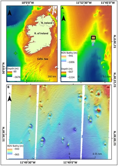
Figure 1.
(A) Study site area. The bathymetry acquired in the downslope Moira Mounds region derived from remotely operated vehicle (ROV) based multibeam echosounder (MBES) data displaying the extent of (B) outlined in black, (B) moated cold-water coral mounds surrounded by mobile sediment worked into sediment waves. Coral ridges appear immediately south of the larger mounds.
2. Materials and Methods
2.1. Multibeam Echosounder Data Acquisition and Processing
The MBES data were collected using a Kongsberg EM2040 mounted to the Holland 1 ROV operating at a frequency of 300 kHz as part of the QuERCI survey in 2015 aboard the RV Celtic Explorer [54]. The survey altitude was maintained at 150 m and was recorded using the ROV altimeter. The navigation and positioning were acquired using a Sonardyne USBL and a 1200 kHz RDI workhorse DVL beacon and were corrected using a Kongsberg HAINS (INS) system. Raw MBES data were sorted as *.all file formats and imported into Qimera processing software to manually remove any erroneous data using the swath editor tool [55]. Horizontal and vertical offsets within the data were removed using the horizontal shift tool and the varying vertical shift tool in Qimera [55]. A cross check analysis was applied to these data to determine the accuracy of the bathymetric data processing against the processing standards set by the International Hydrographic Organisation (IHO) [56]. These data were gridded at 1 m resolution and exported into an ArcGRID *.asc file format. All bathymetric data were imported into ArcGIS 10.6 to derive bathymetric derivatives (Table 1). The slope, aspect, sinaspect, cosaspect, and variance were calculated using the benthic terrain modeler 3.0 toolbox in ArcGIS 10.6 [57]. The bathymetric position index (BPI) was generated at 2 separate scales using the equation outlined below:
where Zgrid is the bathymetric data [58]. The focalmean derives the mean of the bathymetric data within a circle shaped kernel of radius r, this was completed in the focal statistics tool in the neighbourhood toolset in ArcGIS 10.6. The radius of the kernel determines the scale of the BPI. The BPI layer was then created by subtracting the mean bathymetric layer from the Zgrid, this was completed in the raster calculator tool in the map algebra toolset in ArcGIS 10.6.

Table 1.
Image layers used for segmentation in eCognition Developer.
2.2. Object-Based Image Analysis
2.2.1. Morphological Characterisation
Segmentation is a semi-automated process by which an image is separated into discrete image objects and is the first step in object-based image analysis (OBIA) [39,59]. The effectiveness of object based image analysis is predicated on the efficacy of the segmentation in demarcating the features of interest [60]. In this paper, the segmentation was deployed as a hierarchal process, to distinguish between features that exhibit a significant disparity in scale and characterise their morphology. This morphological characterisation was performed over a series of four phases that were adapted from Summers et al. [61] (Figure 2). These phases utilise the multiresolution segmentation algorithm (MRS), the spectral difference algorithm, and the pixel base object resizing algorithm, which are all found within the eCognition Developer processing suite [62]. The MRS algorithm groups pixels together into image objects using a predefined homogeneity value that ceases the amalgamation of pixels once this value is met, this homogeneity value is defined as the scale parameter [62,63]. Moreover, the influence of image object shape on the segmentation is controlled by the shape parameter, the smoothness of the image object outline created by the segmentation is regulated by the compactness factor [64]. An ideal segmentation presents an accurate reflection of the outline of the targets of interest [60,65,66]. However, this is seldom the case, with many features of heterogeneous classes occurring within the same image object (under segmentation), or one feature being demarcated by multiple image objects (over segmentation) [67]. Amalgamation of neighbouring image objects can be completed using the spectral difference algorithm, where image objects are merged if the difference between mean layer intensities is below a user defined value [62]. The pixel-based object resizing algorithm can contract or expand image object boundaries until a specific geometry has been achieved or image layer value has been met [68].
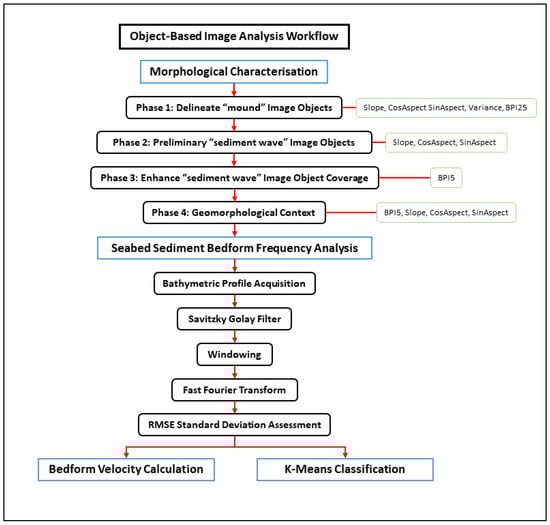
Figure 2.
Workflow chart detailing the separate phases for the morphological characterisation, outlined in black and the image layers deployed during this section, outlined in green. The steps required for the seabed sediment bedform frequency analysis are also mapped out, with the outputs of this analysis feeding into the bedform velocity calculation and the k-means classification.
In the first phase, the MRS algorithm was deployed on the cosaspect, sinaspect, slope, and variance image layers with a scale parameter of 10, a shape factor of 0.1, and a compactness factor of 0.1. Any image object with a mean BPI25 of ≥100 standard of a deviation of BPI25 were merged using the spectral difference algorithm. This algorithm merges adjacent image objects if the difference in mean image layer values between the image objects is below a defined threshold [62]. Slope, sinaspect, and cosaspect were the image layers included in this process and a maximum spectral threshold value of 12 was chosen. A second iteration of the spectral difference algorithm was applied to image objects with a mean BPI25 value of <100% of a standard deviation of BPI25. This combination of algorithms provided preliminary outlines of large-scale features such as the coral mounds and their surrounding moats. Thus, a classification was developed to add geomorphological context for these two larger scale features. “Mound” image objects—hereafter described as “mounds”—were identified as positive topographical features depicted in the BPI25 image layer. “Moat” image objects—hereafter described as “moats”—were identified as negative topographical features depicted by the BPI25 image layer. Any image object with a mean BPI25 value of >50% of a standard deviation of BPI25 was classified as a “mound”. The pixel-based image object resizing algorithm was deployed to improve the accuracy of the “mounds” by expanding their borders until a threshold of >12.5% of a standard deviation of BPI25 was met. Any image object with a mean BPI25 value of <−50% of a standard deviation of BPI25 was classified as a “moat”. The pixel-based image object resizing algorithm was deployed to improve the accuracy of the “moats” by expanding their borders until a threshold of <−12.5% of a standard deviation of BPI25 was met.
Phase two of the morphological characterisation process was deployed on the remaining “unclassified” image objects to delineate regions that potentially represented SSBs. The MRS algorithm was used to segment the sinaspect and cosaspect layers with a scale parameter of 3, a shape parameter of 0.1, and a compactness factor of 0.1. These initial image objects were merged using the spectral difference algorithm on the cosaspect and sinaspect layers with a maximum spectral difference threshold value of 0.3. A “sediment waves” class was assigned to image objects that represented SSBs. To execute this classification, a hue-saturation-value (HSV) colour transformation was employed to help capture truncated image objects with a common slope direction. This colour transformation was applied twice, once with an image layer configuration of slope as red, cosaspect as green, and sinaspect as blue, and a second time with slope as red, sinaspect as green, and cosaspect as blue. Any image object with a HSV value derived from the first image layer configuration of ≥0.9 and a border length/area of 0.32 were classified as “sediment waves”. Any image object with a HSV value derived from the second image layer configuration of ≥0.9 and a border length/area of 0.32 were classified as “sediment waves”.
During phase three, “sediment waves” image object boundaries were adjusted over several iterations to provide a more accurate representation of these. Summers et al. [61] identified BPI5 as the most appropriate image layer for accurately identifying the extent of SSBs. Accordingly, the BPI5 image layer was used here with the pixel-based object resizing algorithm to improve the coverage of SSBs by “sediment waves”. All “sediment waves” were grown until a threshold of >12.5% of one standard deviation of BPI5 had been met. A second implementation of this algorithm grew the “sediment waves” until a threshold of <−12.5% of a standard deviation of BPI5 was met. Any inset “unclassified” image objects found within the “sediment waves” were removed by shrinking the “unclassified” image objects using the pixel-based object resizing algorithm. The candidate surface tension parameter was used as the criterion for this contraction. This parameter creates a square that is defined in image pixels by the user and determines the relative proportion of the classified pixels within this square. Any portion of an inset image object that had <40% labelled as “unclassified”, the resulting portion of that inset image object would be shrunk. Be replaced with an “intermediate” class, if this “intermediate” image object shared ≥65% of its border with “sediment waves” and if the border length/area was ≥0.35, then it would be classified as a “sediment wave”. Any remaining “intermediate” image objects were redesignated as “unclassified” image objects.
Phase four of the morphological characterisation is similar to the third phase detailed in Summers et al. [61]. However, this phase deviates from the previous workflow by using the MRS algorithm to demarcate the individual sediment wave crests and their corresponding troughs. To complete this action the MRS algorithm is deployed separately to segment the “ridge” image objects—hereafter described as “crests”—and the “valley” image objects—hereafter described as “troughs”—by using the cosaspect and sinaspect bathymetric derivatives. The scale parameter, shape parameter, and the compactness factor were set to 12, 0.1, and 0.1, respectively.
2.2.2. Seabed Sediment Bedform (SSB) Frequency Analysis
Upon conclusion of the morphological characterisation, the data were exported as a line shapefile. Any line object that was classified as “crest” was selected for processing. The mean trend for each “crest” line object was acquired using the linear directional mean tool from the spatial statistics toolbox in ArcGIS 10.6 (Figure 3A). The mean compass bearing derived as part of this analysis was integrated with the “crest” line objects to bestow them with the trend direction. A perpendicular line was generated extending 50 m from either side of each line object to avoid geometrical distortions introduced by measurements taken at oblique cross sections (Figure 3B) [69]. This length was chosen as it exceeded the maximum perceived wavelength of all SSBs within the area [69]. The bathymetric profile was extracted at every metre along the perpendicular line, corresponding with the minimum horizontal spatial resolution achievable with these data. As two separate principal SSB orientations were observed in the region, the data were separated by the orientation values after classification.
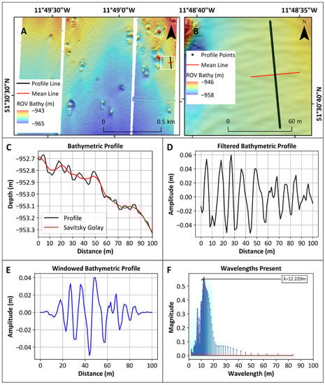
Figure 3.
Displaying (A) an example of a mean line, its corresponding perpendicular and the extent of (B) outlined in white, (B) the points generated along the perpendicular line (C) the bathymetric profile extracted from the bathymetry with a profile generated by a Savitzky Golay filter with a chosen window of 21 and a polynomial value of 3, (D) the bathymetric profile after the subtraction of the Savitzky Golay filter profile, (E) the filtered bathymetric profile with a window function applied, and (F) a Fast Fourier Transform of the windowed profile providing a spectral view of the wavelengths present in the profile after the removal of the Savitzky Golay filter.
Contemporary research has deployed fast Fourier transformations (FFTs) to deliver spatial series information on profiles derived from SSBs [41,70,71,72]. This technique provides the capacity to derive the number of SSBs over a defined interval of space, represented as wavenumber, and the space between each individual SSB, defined as wavelength [73]. Therefore, after acquisition of the bathymetric profile data had been achieved, they were imported into a pythonic coding environment to apply a FFT to extract the wavelength and wave height of each sediment wave. This workflow was executed using the numpy library in Python 3.7 [74]. An effective FFT approach requires the data to meet certain prerequisites including stationarity [75]. Stationarity is a property of the data that asserts that a superimposed trend is not present, and that the wavenumber content remains constant along the length of the appraised profile [75,76]. Here, this stationarity was assessed using an augmented Dickey–Fuller (ADF) unit root test [77]. As many of the SSBs were found to occur on larger scale slope features, detrending techniques were deployed to ensure stationarity was achieved [78,79]. Thus, preventing these regional low frequency slopes from dominating the analysis and obfuscating the local wavenumber value [76]. The Savitsky Golay filter was deployed to achieve this, which fits data points contained within a moving window to a polynomial [80,81,82]. Several values for moving window size were assessed in each instance, with the window size set at 10 step intervals ranging from 21 to 101. The window size chosen was the one that achieved stationarity and the lowest combined root mean square and standard deviation values and was subtracted from the bathymetric profile (Figure 3C,D). Another assumption of FFT is the presence of an integral number of SSBs within the analysis [75]. Data that fail to fulfil this condition can introduce spectral leakage into the analysis, where many additional wavenumbers occur adjacent to the high amplitude peaks [78]. The solution was to window the SSB profile, which ensures that the edges of the sample taper to 0 m and an integral value of wavelength is achieved (Figure 3E) [70,78]. After windowing, the data were then zero padded to ensure that the associated wavenumber is more resolvable in the spectral profile. FFT was applied to the data after zero padding had been completed. Once achieved, the wavenumbers that were derived were limited to below 0.01 m−1 to further exclude any large profiles. The wavenumber with the highest spectrum value from this subset was converted to wavelength in each instance (Figure 3F). Any SSB profile that failed to achieve stationarity after the initial processing were filtered at a moving average of 11 to capture regional slopes with a higher wavenumber. If this failed to achieve the stationarity, then the SSB was designated a wavelength and wave height value of 0. The Nyquist interval is the minimum measurable wavelength discernible within a dataset, this was obtained by doubling the sampling resolution of the data [70].
2.2.3. K-Means Classification
K-means classification separates the objects into a group or cluster with a similar data profile while ensuring that the object is sufficiently distinct from other groups in the analysis [83]. The number of clusters employed is user defined by determining the cluster with the lowest Euclidean distance from its cluster centre to the object within the multi variant data space [84]. Initially these cluster centres are randomly distributed. Data are categorised by bestowing the class of the closest cluster centre [85]. The positions of these cluster centres are optimised by discerning the centre configuration with the lowest aggregated squared error in n-dimensional space, with n corresponding to the number of variables included [84,85,86]. K-means clustering is the most common clustering technique due to its simplicity and effectiveness and is frequently used to partition marine environmental data [85,86,87].
Upon morphological characterisation of the data, the image objects were exported as a polygon shapefile. Any image object classified as “crest” was selected as an input for the k-means classification, the remaining image objects were excluded (Figure 4). The wavelength for each “crest” derived during the seabed sediment bedform frequency analysis were added to the shapefile attributes. All “crest” image objects were imported into a python coding environment to classify them based on morphology, spatial density, and mean bathymetric derivatives (Table 2). Values 2 to 8 were assessed for values for k by comparing their respective inertial values, which represents the sum of squared distances of the samples to their closest cluster centre [88]. The value of k found before a significant change in the slope of inertia values will be deemed the most appropriate value for k. As, this would indicate the effective clustering of the morphologies displayed by the “crests” while maintaining the minimum number of classes required to describe the data. A separate class density distribution layer was derived for each k-means class. Calculating the density of the features as points for each class over a defined pixel neighbourhood (75 m) with density being displayed as number of class point features per km2. Geometrical features available in eCognition were derived from the image objects and were the principal component to the classification, all features used in the k-means classification are outlined in Table 2. The features that displayed the greatest degree of inter class variation were used to reconcile the k-means classification to the environment from which they were derived.
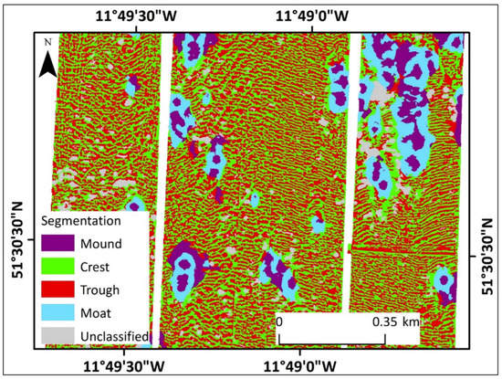
Figure 4.
Displaying the multi-scale morphological characterisation output with the larger scale coral mound features—the “mounds” and “moats”—and the lower scale features—the “crests” and “troughs”.
Table 2.
Image object features employed in the k-means classification and their respective feature categories.
2.3. Bedform Velocity Calculation
Current speed calculations were based on the bedform velocity matrix presented by Stow et al. [42]. Stow et al. [42] delineated transverse bedforms into 6 separate categories including ripples, sinuous dunes, barchanoid dunes, sand waves, gravel waves, and giant sediment waves (mud waves). These categories are defined using the wavelength, wave height, and the sinuosity of the bedform. Furthermore, each category is given a corresponding minimum and maximum current velocity. In our study, we established individual multiple linear regression using the ranges for wavelength, wave height, and current velocity provided by Stow et al. [42] for each SSB category. With wavelength and wave height as the explanatory variables and current velocity as the response variable. The resultant wavelengths and wave heights obtained from the FFT workflow outlined above were used to identify each “crest” as one of these transverse SSB categories. Once labelled, a predicted velocity was derived for the “crest” using the regression model developed for that category. Median values for current speed were obtained for each k-means class separately at ≤25 m, ≤50 m, ≤100 m, ≤150 m, and ≤200 m distances from the “mounds” to observe any relationships between current speed variation and proximity to “mounds”. Median values were also obtained for each class for the 2 dominant SSB orientations. Furthermore, current orientations were derived for each k-means class at ≤25 m and ≤200 m from “mounds” to determine any potential influences the CWC mounds may have on current orientation. Median values for current orientation were also derived at these distances for each k-means class.
3. Results
3.1. Multibeam Cross Check Analysis
Cross checking revealed that these MBES bathymetry data achieved the IHO special order standard for accuracy of bathymetric data.
3.2. Morphological Characterisation
The median area for “crests” was 140 m2. The median curvature to length value was 7.80 and the median length to width value was 2.31.
3.3. Fast Fourier Transform and SSB Frequency Analysis
Three SSB categories were observed within the “crests”, sediment ripples, sinuous dunes, and sand waves. Forty-eight “crests” exceeded the filter parameters and thus were designated a wave height and wavelength of 0 m. The minimum sampling interval observed was 2 m.
3.4. Classification
A 5 k-means clustering was chosen as it occurred before a significant local variation in the inertial value slope (Figure 5A,B). Class 0 had the highest median length/width of 3.62 m, and the largest areal extent with a median area of 233 m2. This class exhibits a low sinuosity with the second lowest median curvature/length value of 6.34°. Median wave height for these objects was the second highest observed at 0.315 m. The median wavelength for these image objects was the shortest for any class at 11.29 m. These image objects had a mean slope of 1.47°. Class 1 is the second most linear with a median length/width of 2.79 m and a moderate areal extent with a median value of 155 m2. This class exhibits a low sinuosity with the lowest median curvature/length value of 6.29°. These image objects had a mean slope of 1.46°. Class 2 had the lowest length to width ratios with a median value of 1.65 m. It also had the lowest median areal extent (90 m2). This class had the second highest median curvature/length at 9.72° and the second lowest mean slope at 1.39. This class also had a median wave height of 0.293 m. Class 3 had a low median length/width of 1.93. They also had the second lowest median area value at 114 m2. This class had the highest median curvature/length value length at 10.35°. These image objects a mean slope of 1.31°. Class 4 had the highest median wavelength value recorded at 12.43 m and the lowest median wave height value at 0.128 m. These image objects had moderate median curvature/length and length/width values of 7.15° and 1.93 m, respectively. These image objects had a mean slope of 3.27°. Further median values for each k-means class are provided in Table 3.
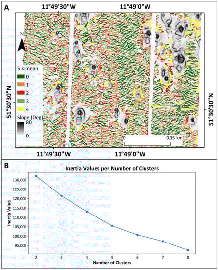
Figure 5.
Displaying (A) the slope image layer and the product of the 5 k-means classification of morphology, spatial density, and mean bathymetric derivative, (B) inertial values for each value of k.
Table 3.
Median area, length/width, curvature/length, mean slope, and wave height for each class.
6605 “crests” were orientated from south-west to north-east, 5105 “crests” were orientated from south-east to north-west. Furthermore, 64% of all “crests” that were classified as class 0 and 58% of “crests” that were classified as class 1 are orientated to the north-east.
3.5. Current Velocity Analysis
A bimodal distribution in current speeds was identified occurring throughout the study site with a mean current speed of 0.37 m s−1 (Figure 6A). Therefore, the “crests” were separated into 2 groups: >0.40 m·s−1 (the fast group abbreviated to FG), and ≤0.40 m·s−1 (the slow group abbreviated to SG) to ensure successful production of summary statistics for each mode. The median current speed for all SG “crests” was 0.28 m·s−1 and the median current speed for all FG “crests” was 0.60 m·s−1. When comparing the median current speeds taken at ≤25 m from “mounds” and median current speeds taken at ≤200 m from “mounds”, an increase current speed with increasing distance away from the “mounds” was noted. For instance, the SG “crests” displayed a consistent increase in current speed across the 2 chief orientations with increasing distance from the “mounds” (Figure 6B,C). The north-north-west aligned SG “crests” showed an increase in median current speed for all 5 classes when comparing median current speeds acquired at ≤25 m and ≤200 m from the “mounds”. Class 0 showed an increase in median current speed of 0.013 m·s−1 from 0.266 m·s−1 to 0.279 m·s−1. Class 1 exhibited an increase of 0.007 m·s−1 from 0.273 m·s−1 to 0.280 m·s−1. Class 2 displayed a rise in median current speed of 0.007 m·s−1 from 0.269 m·s−1 to 0.276 m·s−1. Class 3 showed an increase in median current speed of 0.006 m·s−1 from 0.271 m·s−1 to 0.277 m·s−1. Class 4 exhibited a rise in median current speed of 0.002 m·s−1 from 0.26 m·s−1 to 0.262 m·s−1.
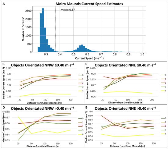
Figure 6.
(A) Current speed values for all “crests”, median current speed values for (B) north-north-west aligned slower group (SG) “crests”, (C) north-north-east aligned SG “crests”, (D) north-north-west aligned faster group (FG) “crests”, (E) north-north-east aligned FG “crests”.
The SG image objects orientated to the north-north-east displayed an increase in median current speeds when comparing median current speeds taken at ≤25 m and ≤200 m from the “mounds” in 4 of 5 classes. Class 0 displayed an increase in median current speeds of 0.012 m·s−1 from 0.268 m·s−1 to 0.280 m·s−1. Class 1 displayed an increase in median current speeds of 0.014 m·s−1 from 0.266 m·s−1 to 0.280 m·s−1. Class 2 exhibited an increase in median current speeds of 0.001 m·s−1 from 0.277 m·s−1 to 0.278 m·s−1. Class 3 displayed an increase in median current speeds of 0.014 m·s−1 from 0.266 m·s−1 to 0.280 m·s−1. Conversely, class 4 exhibited a decrease in median current speeds of 0.0002 m·s−1 from 0.264 to 0.263 m·s−1.
The FG image objects orientated north-north-west have the largest increase in median current speeds between these distance intervals from the “mounds”. Four of the 5 k-means classes contained in the FG “crests” mode exhibit an increase in median current speed between the ≤25 m and ≤200 m distance intervals from the “mounds”. For instance, the FG objects assigned to class 0 and aligned to the north-north-west experienced an increase in median current speed of 0.033 m·s−1 from 0.542 m·s−1 m to 0.575 m·s−1. Class 1 from the same orientation and current regime also experienced an increase in median current speed of 0.034 m·s−1 from 0.543 m·s−1 to 0.577 m·s−1. Class 2 “crests” from this subset exhibited a smaller increase in current speed of 0.006 m·s−1 from 0.559 m·s−1 to 0.565 m·s−1. An increase in current speed of 0.030 m·s−1 from 0.530 m·s−1 to 0.560 m·s−1 was observed for class 3 “crests”. Conversely, class 4 for the same orientation and current regime experienced a decrease in median current speed of 0.023 m·s−1 from 0.571 m·s−1 to 0.548 m·s−1.
For the north-north-east aligned FG “crests”, 2 classes exhibited an increase in median current speed. Class 0 had an increase in median current speed of 0.006 m·s−1 from 0.564 m·s−1 to 0.570 m·s−1. Class 1 had an increase in median current speed of 0.021 m·s−1 from 0.556 m·s−1 to 0.577 m·s−1. Three classes aligned north-north-east in the FG current regime have shown a decrease in current speed. Class 2 had a decrease in median current speed of 0.026 m·s−1 from 0.590 m·s−1 to 0.564 m·s−1. Class 3 displayed a decrease in median current speed of 0.002 m·s−1 from 0.56 m·s−1 to 0.558 m·s−1. Class 4 exhibited a decrease in median current speed of 0.001 m·s−1 from 0.545 m·s−1 to 0.544 m·s−1 (Figure 6B–E).
Moreover, when comparing the relative proportion of FG “crests” versus SG “crests” at the same distance intervals relative to the “mounds”, an increase in the proportion of FG “crests” was observed in both orientations. An increase of 11.4 percentage points from 15.6% to 27.0% was noted for “crests” orientated to the north-north-west (Figure 7A). A smaller increase in the proportion of FG “crests” orientated to the north-north-east was noted with an increase of 4.5 percentage points from 23.3% to 27.8% (Figure 7B).
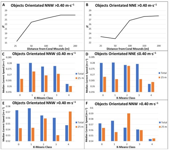
Figure 7.
The proportion of FG “crests” over distance from the “mounds” for (A) north-north-west aligned “crests”, (B) north-north-east aligned “crests”, and a comparison of median current speeds for each class taken at ≤25 m from the “mounds” and the whole dataset for (C) all north-north-west aligned SG “crests” (D) north-north-east aligned SG “crests”, (E) north-north-west aligned FG “crests”, (F) north-north-east aligned FG “crests”.
An increase in median current speeds was observed for all k-means classes when comparing the median current speed per class acquired at ≤25 m away from the “mounds” and the median current speed per class for all SG “crests” aligned to the north-north-west (Figure 7C). The largest increase was observed for class 0 at 0.013 m·s−1. Similarly, an increase in median current speeds per k-means class was observed for 4 of the 5 classes when comparing the median current speed per class acquired at ≤25 m away from the “mounds” and the median current speed per class acquired for all SG “crests” aligned to the north-north-east. The largest increase was observed for class 1 at 0.014 m·s−1 (Figure 7D). A decrease of 0.00173 m·s−1 was noted for class 4. There was an increase in median current speeds for 4 of the 5 k-means classes when comparing the median current speed per class acquired at ≤25 m away from the “mounds” and the median current speed per class for all FG “crests” aligned to the north-north-west (Figure 7E). The largest increase was observed for class 1 at 0.034 m·s−1. A decrease of 0.023 m·s−1 was observed for class 4. There was an increase in median current speeds for 3 of the 5 k-means classes noted when comparing the median current speed per class acquired at ≤25 m away from the “mounds” and the median current speed per class for all FG “crest” “class aligned to the north-north-east. The largest increase in median current speed was observed for class 1 at 0.020 m·s−1. The largest decrease in median current speed was observed for class 3 at 0.026 m·s−1.
Current speed and current direction were extracted for each class image object at ≤25 m and ≤200 m away from the “mounds” (Figure 8A–J). However, as the direction derived from the linear directional mean tool was ambiguous when observed in the full 360° range 180° was subtracted from all direction values above 180°, allowing for separation between the 2 dominant SSB orientations. Thus, any “crest” with orientation values occurring between 0° and 90° represent those SSBs whose crests aligned to the north-north-west. Any “crest” with orientation values occurring between 90° and 180°represent SSBs whose crests were aligned to the north-north-east. The median current orientations acquired at ≤200 m from the “mounds” for classes 0, 1, 2, 3, and 4 aligned to the north-north-west were 340°, 342°, 327°, 332°, and 329°, respectively. The median current orientations acquired at ≤25 m from the “mounds” for classes 0, 1, 2, 3, and 4 with the same alignment were 325°, 341°, 322°, 321°, and 325°, respectively. A bimodal distribution of current flow was noted for class 0 at ≤200 m from the “mounds” however, this was not noted for any of the other k-means classes. The median current orientations acquired at ≤200 m from the “mounds” for classes 0, 1, 2, 3, and 4 aligned to the north-north-east were 20°, 19°, 29°, 29°, and 28°, respectively. The median current orientations acquired at ≤25 m from the “mound” image objects for classes 0, 1, 2, 3, and 4 with the same alignment were 28°, 24°, 37°, 33°, and 20°, respectively.
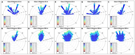
Figure 8.
Polar plots indicating current speed and orientation for (A) class 0 ≤25 m proximity to the “mounds”, (B) class 1 ≤200 m proximity to the “mounds”, (C) class 1 ≤25 m proximity to the “mounds”, (D) class 1 ≤200 m proximity to the “mounds”, (E) class 2 ≤25 m proximity to the “mounds”, (F) class 2 ≤200 m proximity to the “mounds”, (G) class 3 ≤25 m proximity to the “mounds”, (H) class 3 ≤200 m proximity to the “mounds”, (I) class 4 ≤25 m proximity to the “mounds”, (J) class 4 ≤200 m proximity to the “mounds”.
Density distribution layers reveal that the greatest density of class 0 occurs to the north-east of the study site (Figure 9A). The greatest density of class 1 occurs to the centre and south of the study site (Figure 9B). The greatest density of class 2 and 3 occurs to the east and north-west (Figure 9C,D). Class 4 “crests” occur in greatest density to the north-east directly surrounding the CWC mounds in this area (Figure 9E).
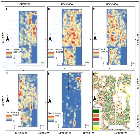
Figure 9.
5 k-mean class density maps for each class: (A) class 0, (B) class 1, (C) class 2, (D) class 3, and (E) class 4 displaying the extent of (F) outlined in black, (F) displays the k-means classification for the “crests” in the north-western portion of the study site.
4. Discussion
4.1. K-Means Classification of Sediment Bedform Type
A five k-means classification produced a robust identification of transverse SSB types separating each class chiefly by linearity, sinuosity, and areal extent (Table 4). Linearity and sinuosity in this classification are depicted by the values for length/width and curvature/length. Higher length/width and lower curvature/length values designate greater SSB linearity. Lower length/width and higher curvature/length values reveal increased SSB sinuosity. Sinuosity gradually increased from class 0 to class 3, with class 0 representing large straight SSBs and class 3 representing medium sinuous SSBs (Table 4). A slight decrease in median current speed was observed for classes 2 and 3—small and medium sinuous SSBs—when comparing them with classes 0 and 1—large and medium straight SSBs (Figure 7C–F). Therefore, the increase in sinuosity observed for the medium and small sinuous SSBs is not due to an increase in current speed, rather this increase in sinuosity is a result of the superimposition of one or more sets of bedforms onto another. Large straight SSBs represent the most linear SSBs that occur in regions of local unidirectional flow. Furthermore, the unidirectional flow denoted by this category is supported by the clear bimodality of the current flow orientations acquired for these SSBs at ≤200 m proximity to the “mounds” (Figure 8B). Few intermediate current flow orientations occur between these two modes, indicating the presence of two dominant current regimes, one flowing to the north-north-east, and the other flowing to the north-north-west. This bimodality is not detected at ≤200 m proximity to the “mounds” for any of the other SSB categories. Hence, this suggests an increase in interference between the two dominant current regimes for each of the remaining categories. Moreover, this interference is most pronounced in the small and medium sinuous SSBs, where SSBs exhibit a greater level of sinuosity and thus, a greater degree of SSBS superimposition. Class 4—medium obstructed SSBs—are SSBs adjacent to CWC mounds, whose wave heights are reduced due to the obstruction in current flow created by the CWC mounds. Consequently, these SSBs consistently have the lowest median current speed (Figure 7C–F).
Table 4.
Reconciliation of k-means classes to environmental categories complete with a brief interpretation.
4.2. Regional, Local and Micro Hydrodynamics
This study site occurs between 941 and 1006 m depth which is within the MOW water mass which generates northerly flowing contour currents that are influenced by tidal rectification processes [47,49,51]. Dorschel et al. [51] observed north-north-west migrating sediment waves to the east of the nearby Galway Mound postulated that the regional geostrophic contour currents were chiefly responsible for their formation. Given that the north-north-west aligned currents observed here align with these findings, the associated bedforms are considered to have a similar origin. However, this does not explain the clear presence of a north-north-east current regime within this region. The density of distribution of each of the SSB categories can be used as a surrogate for the consistency of local current flow. An increase in the density of medium and small sinuous SSBs can be found to the east and north-east of the study site, this increase implies an increase in the inconsistency of the current flow within this portion of the site. Moreover, this increase occurs as the site approaches the margin of the blind channel (Figure 1A), suggesting that the topographical effects of the channel margin cause this disruption. Consequently, the north-north-east aligned flow may be due to the local topographical steering of the contour currents by the channel margin. Additionally, the presence of the large linear SSBs to the north-west of the study site coincides with the centre of the channel and may signify a decrease in the disruption of the contour currents, leading to more consistent unidirectional flow (Figure 8F). This is also supported by the larger proportion of north-north-west aligned large linear SSBs to the west of the region. This local increase in unidirectional flow to the north-west of the study site also corresponds with the greatest density of mounds reported by Lim et al. [14], suggesting that this type of flow is more favorable for CWC growth. This may explain the decrease in mound density to the east of the site, where greater disruption of currents occurs. Therefore, the interaction of the regional MOW tidally influenced contour currents coupled with the local topographical steering by the blind channel may be the cause of the bimodal distribution of current flow direction.
A change of >7° in median current direction is observed for both dominant current regimes when comparing the orientations of the current flow acquired within ≤25 m of the “mounds” and ≤200 m to the “mounds” for large linear SSBs and small sinuous SSBs (Figure 8A,B,E,F). This suggests that current flow for both current regimes is refracted as it approaches the “mounds” thus, demonstrating topographic steering that is proximal to the “mounds” where topographical steering occurs on a micro scale directly surrounding the “mounds”. Nevertheless, this topographic steering is not as apparent when observing the smaller coral mounds, suggesting larger mounds have a more profound influence on the current regime, this is in agreement with the analysis conducted by Lim et al. [14].
In addition to the current orientation, a bimodal distribution of the current speed values is also evident (Figure 6A). The >0.40 m·s−1 FG mode is significantly lower than the ≤0.40 m·s−1 SG mode suggesting that these higher current speeds are locally intensified currents and are not indicative of the prevailing regional current speed. While the mean value for current speed procured for the entire “crest” class may not adequately reflect the overall current speed distribution observed in Figure 6A, it is similar to previous regional current speed estimations for this and nearby areas [14,51]. Moreover, this mean value may demonstrate how current speed estimations derived from a single or limited sediment samples can be misleading and therefore, not a reflection of the significant spatial variations in local current speeds.
4.3. Mound Proximity and SSB Characteristics
The presence of the “moats” surrounding the larger “mounds” illustrates intensive scouring, forming a comet and tail morphology, and is postulated to occur due to high intensity, low frequency north–south cold water cascade events [14]. However, when examining the BPI25 bathymetric derivative layer, we can see that the tails alter direction with movement towards the east and north-east of the study site (Figure 10). This change in tail orientation coincides with the increase in density of medium and small sinuous SSBs, indicating an increased disruption of current flow potentially attributable to the local topographic steering imprinted by the approach to the channel margin [26]. The resulting current flow would become more aligned with the CWCs occurring on slopes orientated to the SW, exposing the CWCs on slopes orientated to the NE to more erosive conditions that are unfavorable to CWC growth. Conversely, a consistent reduction in the median current speed is observed with increasing proximity to the mounds for each of the SSB categories. For instance, the lowest current speeds for each SSB category for the north-north-west aligned “crests” are found within ≤25 m of the “mounds”. This is consistent for the SG and the FG “crests” except for the FG medium obstructed SSBs. Additionally, the declining proportion of FG SSBs with increasing proximity to “mounds” for the north-north-west SSB orientation further indicates the deceleration of current speed.
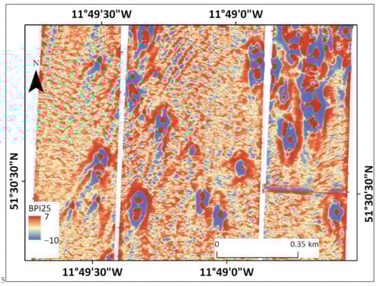
Figure 10.
BPI25 bathymetry derivative layer displaying the intense scouring as negative topographic features surrounding the CWC mounds forming a comet and tail morphology.
However, the decline of current speed is not equal across the two dominant current orientations. What is evident is a slight decline in the current speed values for the SG and FG SSBs orientated to the north-north-east, however this decline is not as significant as those orientated to the north-north-west. Moreover, the proportion of FG SSBs orientated to the north-north-east remain relatively consistent with proximity to the “mounds”. Suggesting that the currents originating from the south-south-west are not impeded as much as their south-south-eastern counterparts. This direction specific obstruction may be influenced by the intensely scoured moats, causing increased erosion of CWC framework, and removing a portion of the obstruction that they provide on north-east aligned slopes. These findings are reflected by Conti et al. [26] who note that live coral framework mainly occur on the north of Piddington Mound across two main slope orientations, at 300° and 70°, with most of the live coral framework occurring on slopes with an orientation of 300°. The diminished presence of CWCs on the north-eastern side of the Piddington Mound may indicate that the conditions imposed by the postulated cold water cascade events may prevent effective growth of CWCs for slopes with this orientation or that regular current speeds are too high for corals to thrive. The reported mean slope value of 300° is shallower than the north-north-west current flow direction derived at ≤200 m from the “mounds” for all SSB categories. However, the slightly shallower median direction of the current flow observed at ≤25 m to the “mounds” suggests that currents slow down and alter direction upon approach to the “mounds”. These micro scale topographic steering forces imprint a better alignment with the live coral framework. Moreover, the slower current speeds proximal to the “mounds” encourage better conditions for food capture (Figure 8A–J).
4.4. Implications
Lim et al. [15] demonstrated the use of acoustic Doppler current profiler (ADCP) derived hydrodynamic data in augmenting the interpretative capabilities of high resolution semi-automated classification of CWC environments. Here, we have provided a means of estimating the current speed from bathymetric data without the use of ADCP instrumentation that is largely congruent with their findings. Furthermore, ADCP deployment offers the opportunity for finer calibration of this technique, enabling the direct extrapolation of knowledge deduce from ADCP current data from individual points to entire bathymetric mosaics. Future research could focus on implementing this strategy to provide a more robust current speed estimation. The OBIA morphological characterisation employed with this classification scheme has been proven to be robust to significant disparities in spatial resolution, making this technique flexible to a wide range of scales [61]. Such properties render this technique an essential mechanism to produce multi scale seabed habitat maps for MPA management and monitoring, logistics for offshore physical infrastructure [25].
On a broader scale, the method described can be used to quickly derive objective, allogenic environmental information from bathymetric data. This can subsequently be used in maritime industrial development, environmental impact assessments as well as preliminary desktop studies. With large scale datasets now readily available, such methods can simply be applied by non-experts. Digital elevation models (DEMs) and sedimentary bedforms are not unique to the marine realm and as such, the workflow presented here could be used to integrate terrestrial DEM data, promoting the potential of a seamless geomorphological habitat map [89]. Furthermore, such workflows could be applied to extraterrestrial settings, where seafloor bedforms provide an excellent analog for thick atmosphere environments [90].
5. Conclusions
This research has established the first OBIA workflow that can provide an indication of the consistency, direction, and velocity of the hydrodynamic regime directly above the seafloor solely using MBES bathymetry data. Our findings have wide applications but are used here to report that CWC growth in the downslope Moira Mounds area was shaped by regional north-north-west aligned geostrophic contour currents induced by the MOW that were influenced themselves by local and micro topographic features. Local topographic steering resulted in the disruption of the contour current flow with approach to the channel margin, resulting in the presence of a bimodal distribution of current flow direction throughout the area. This bimodal current direction corresponds with the two predominant CWC slope orientations found within the region [26]. Moreover, geomorphological characterisation of the SSBs provided a proxy to define regions of consistent unidirectional flow. Previous observations on CWC mound spatial density within this region indicates that the CWC mounds occur in the greatest densities in regions with consistent unidirectional flow [14]. While micro topographic steering forces resulted in the decrease of current speeds with increasing proximity to the CWC mounds. Furthermore, these micro topographic steering forces imprinted a current direction that was more aligned with CWC occurring on slopes facing away from the prevailing current direction, congruent with findings acquired in other CWC mound regions. These results underline the capacity of this approach to derive qualitative data on hydrodynamic regimes on the seabed surface with minimal sampling requirements. Additionally, this technique can be reconciled with current measurements taken from in situ monitoring equipment such as ADCPs to ensure a more effective hydrodynamic regime appraisal.
Author Contributions
Conceptualisation, G.S. and A.L.; Methodology, G.S. and A.L.; Software, G.S.; Validation, G.S.; Formal Analysis, G.S.; Investigation, G.S.; Resources, G.S. and A.L.; Data Curation, G.S. and A.L.; Writing—Original Draft Preparation—G.S.; Writing—Review and Editing, G.S., A.L. and A.J.W.; Visualisation, G.S.; Supervision, A.L. and A.J.W.; Project Administration, A.J.W.; Funding Acquisition, A.J.W. All authors have read and agreed to the published version of the manuscript.
Funding
This research was developed under the Marine Protected Area Management and Monitoring (MarPAMM) (Project IVA5059) supported by the European Union’s INTERREG VA Programme, managed by the Special EU Programmes Body (SEUPB). Holland 1 ROV. RV Celtic Explorer cruises were grant aided by the Marine Institute under the Ship Time Program of the National Development Plan, Ireland. The data processing workflow was developed by Gerard Summers and Aaron Lim is jointly funded by the EU INTERREG V through the Special EU Programmes Body (SEUPB) and the Irish Research Council (Project GOIPG/2015/2700), respectively.
Acknowledgments
Authors would like to thank all cruise crew and scientific parties on RV Celtic Explorer (cruise number CE15009).
Conflicts of Interest
The authors declare no conflict of interest.
References
- Carter, L.; Gavey, R.; Talling, P.J.; Liu, J.T. Insights into submarine geohazards from breaks in subsea telecommunication cables. Oceanography 2014, 27, 58–67. [Google Scholar] [CrossRef]
- Guo, Z.; Hong, Y.; Jeng, D.-S. Structure–Seabed Interactions in Marine Environments. J. Mar. Sci. Eng. 2021, 9, 972. [Google Scholar] [CrossRef]
- Prasad, D.H.; Kumar, N.D. Coastal Erosion Studies—A Review. Int. J. Geosci. 2014, 5, 341–345. [Google Scholar] [CrossRef]
- Degrendele, K.; Roche, M.; Schotte, P.; Van Lancker, V.R.M.; Bellec, V.K.; Bonne, W.M.I. Morphological Evolution of the Kwinte Bank Central Depression before and after the Cessation of Aggregate Extraction. J. Coast. Res. 2010, 77–86. [Google Scholar]
- Wheeler, A.J.; Kozachenko, M.; Masson, D.G.; Huvenne, V.A.I. Influence of benthic sediment transport on cold-water coral bank morphology and growth: The example of the Darwin Mounds, north-east Atlantic. Sedimentology 2008, 55, 1875–1887. [Google Scholar] [CrossRef]
- Roberts, J.M.; Wheeler, A.; Freiwald, A.; Cairns, S. Cold-Water Corals: The Biology and Geology of Deep-Sea Coral Habitats; Cambridge University Press: Cambridge, UK, 2009. [Google Scholar]
- Kenyon, N.H.; Akhmetzhanov, A.M.; Wheeler, A.J.; van Weering, T.C.E.; de Haas, H.; Ivanov, M.K. Giant carbonate mud mounds in the southern Rockall Trough. Mar. Geol. 2003, 195, 5–30. [Google Scholar] [CrossRef]
- Thierens, M.; Browning, E.; Pirlet, H.; Loutre, M.F.; Dorschel, B.; Huvenne, V.A.I.; Titschack, J.; Colin, C.; Foubert, A.; Wheeler, A.J. Cold-water coral carbonate mounds as unique palaeo-archives: The Plio-Pleistocene Challenger Mound record (NE Atlantic). Quat. Sci. Rev. 2013, 73, 14–30. [Google Scholar] [CrossRef]
- Baillon, S.; Hamel, J.-F.; Wareham, V.E.; Mercier, A. Deep cold-water corals as nurseries for fish larvae. Front. Ecol. Environ. 2012, 10, 351–356. [Google Scholar] [CrossRef]
- Roberts, J.M.; Cairns, S.D. Cold-water corals in a changing ocean. Curr. Opin. Environ. Sustain. 2014, 7, 118–126. [Google Scholar] [CrossRef]
- Chapron, L.; Peru, E.; Engler, A.; Ghiglione, J.F.; Meistertzheim, A.L.; Pruski, A.M.; Purser, A.; Vétion, G.; Galand, P.E.; Lartaud, F. Macro- and microplastics affect cold-water corals growth, feeding and behaviour. Sci. Rep. 2018, 8, 15299. [Google Scholar] [CrossRef]
- Boolukos, C.M.; Lim, A.; O’Riordan, R.M.; Wheeler, A.J. Cold-water corals in decline–A temporal (4 year) species abundance and biodiversity appraisal of complete photomosaiced cold-water coral reef on the Irish Margin. Deep Sea Res. Part I Oceanogr. Res. Pap. 2019, 146, 44–54. [Google Scholar] [CrossRef]
- Dorschel, B.; Wheeler, A.J.; Huvenne, V.A.I.; de Haas, H. Cold-water coral mounds in an erosive environmental setting: TOBI side-scan sonar data and ROV video footage from the northwest Porcupine Bank, NE Atlantic. Mar. Geol. 2009, 264, 218–229. [Google Scholar] [CrossRef]
- Lim, A.; Huvenne, V.A.I.; Vertino, A.; Spezzaferri, S.; Wheeler, A.J. New insights on coral mound development from groundtruthed high-resolution ROV-mounted multibeam imaging. Mar. Geol. 2018, 403, 225–237. [Google Scholar] [CrossRef]
- Lim, A.; Wheeler, A.J.; Price, D.M.; O’Reilly, L.; Harris, K.; Conti, L. Influence of benthic currents on cold-water coral habitats: A combined benthic monitoring and 3D photogrammetric investigation. Sci. Rep. 2020, 10, 19433. [Google Scholar] [CrossRef] [PubMed]
- Matos, L.; Wienberg, C.; Titschack, J.; Schmiedl, G.; Frank, N.; Abrantes, F.; Cunha, M.R.; Hebbeln, D. Coral mound development at the Campeche cold-water coral province, southern Gulf of Mexico: Implications of Antarctic Intermediate Water increased influence during interglacials. Mar. Geol. 2017, 392, 53–65. [Google Scholar] [CrossRef]
- Wienberg, C.; Titschack, J.; Frank, N.; De Pol-Holz, R.; Fietzke, J.; Eisele, M.; Kremer, A.; Hebbeln, D. Deglacial upslope shift of NE Atlantic intermediate waters controlled slope erosion and cold-water coral mound formation (Porcupine Seabight, Irish margin). Quat. Sci. Rev. 2020, 237, 106310. [Google Scholar] [CrossRef]
- De Clippele, L.H.; Gafeira, J.; Robert, K.; Hennige, S.; Lavaleye, M.S.; Duineveld, G.C.A.; Huvenne, V.A.I.; Roberts, J.M. Using novel acoustic and visual mapping tools to predict the small-scale spatial distribution of live biogenic reef framework in cold-water coral habitats. Coral Reefs 2017, 36, 255–268. [Google Scholar] [CrossRef]
- van der Kaaden, A.-S.; van Oevelen, D.; Rietkerk, M.; Soetaert, K.; van de Koppel, J. Spatial Self-Organization as a New Perspective on Cold-Water Coral Mound Development. Front. Mar. Sci. 2020, 7, 631. [Google Scholar] [CrossRef]
- Burgos, J.M.; Buhl-Mortensen, L.; Buhl-Mortensen, P.; Ólafsdóttir, S.H.; Steingrund, P.; Ragnarsson, S.Á.; Skagseth, Ø. Predicting the Distribution of Indicator Taxa of Vulnerable Marine Ecosystems in the Arctic and Sub-arctic Waters of the Nordic Seas. Front. Mar. Sci. 2020, 7, 131. [Google Scholar] [CrossRef]
- de Oliveira, L.M.C.; Lim, A.; Conti, L.A.; Wheeler, A.J. 3D Classification of Cold-Water Coral Reefs: A Comparison of Classification Techniques for 3D Reconstructions of Cold-Water Coral Reefs and Seabed. Front. Mar. Sci. 2021, 8, 640713. [Google Scholar] [CrossRef]
- Huvenne, V.A.I.; Bett, B.J.; Masson, D.G.; Le Bas, T.P.; Wheeler, A.J. Effectiveness of a deep-sea cold-water coral Marine Protected Area, following eight years of fisheries closure. Biol. Conserv. 2016, 200, 60–69. [Google Scholar] [CrossRef]
- Coiras, E.; Iacono, C.L.; Gracia, E.; Danobeitia, J.; Sanz, J.L. Automatic Segmentation of Multi-Beam Data for Predictive Mapping of Benthic Habitats on the Chella Seamount (North-Eastern Alboran Sea, Western Mediterranean). IEEE J. Sel. Top. Appl. Earth Obs. Remote Sens. 2011, 4, 809–813. [Google Scholar] [CrossRef]
- Diesing, M.; Thorsnes, T. Mapping of Cold-Water Coral Carbonate Mounds Based on Geomorphometric Features: An Object-Based Approach. Geosciences 2018, 8, 34. [Google Scholar] [CrossRef]
- Savini, A.; Vertino, A.; Marchese, F.; Beuck, L.; Freiwald, A. Mapping Cold-Water Coral Habitats at Different Scales within the Northern Ionian Sea (Central Mediterranean): An Assessment of Coral Coverage and Associated Vulnerability. PLoS ONE 2014, 9, e87108. [Google Scholar] [CrossRef] [PubMed]
- Conti, L.A.; Lim, A.; Wheeler, A.J. High resolution mapping of a cold water coral mound. Sci. Rep. 2019, 9, 1016. [Google Scholar] [CrossRef]
- Calvert, J.; Strong, J.A.; Service, M.; McGonigle, C.; Quinn, R. An evaluation of supervised and unsupervised classification techniques for marine benthic habitat mapping using multibeam echosounder data. ICES J. Mar. Sci. 2014, 72, 1498–1513. [Google Scholar] [CrossRef]
- Janowski, L.; Trzcinska, K.; Tegowski, J.; Kruss, A.; Rucinska-Zjadacz, M.; Pocwiardowski, P. Nearshore Benthic Habitat Mapping Based on Multi-Frequency, Multibeam Echosounder Data Using a Combined Object-Based Approach: A Case Study from the Rowy Site in the Southern Baltic Sea. Remote Sens. 2018, 10, 1983. [Google Scholar] [CrossRef]
- Huvenne, V.A.; Tyler, P.A.; Masson, D.G.; Fisher, E.H.; Hauton, C.; Huhnerbach, V.; Le Bas, T.P.; Wolff, G.A. A picture on the wall: Innovative mapping reveals cold-water coral refuge in submarine canyon. PLoS ONE 2011, 6, e28755. [Google Scholar] [CrossRef]
- Robert, K.; Huvenne, V.A.I.; Georgiopoulou, A.; Jones, D.O.B.; Marsh, L.; Carter, G.D.O.; Chaumillon, L. New approaches to high-resolution mapping of marine vertical structures. Sci. Rep. 2017, 7, 9005. [Google Scholar] [CrossRef]
- Mayer, L.; Jakobsson, M.; Allen, G.; Dorschel, B.; Falconer, R.; Ferrini, V.; Lamarche, G.; Snaith, H.; Weatherall, P. The Nippon Foundation—GEBCO seabed 2030 project: The quest to see the world’s oceans completely mapped by 2030. Geosciences 2018, 8, 63. [Google Scholar] [CrossRef]
- Thorsnes, T. MAREANO–an introduction. Nor. J. Geol. 2009, 89, 3. [Google Scholar]
- Guinan, J.; McKeon, C.; Keeffe, E.; Monteys, X.; Sacchetti, F.; Coughlan, M.; Nic Aonghusa, C. INFOMAR data supports offshore energy development and marine spatial planning in the Irish offshore via the EMODnet Geology portal. Q. J. Eng. Geol. Hydrogeol. 2021, 54, qjegh2020-033. [Google Scholar] [CrossRef]
- Diesing, M.; Green, S.L.; Stephens, D.; Lark, R.M.; Stewart, H.A.; Dove, D. Mapping seabed sediments: Comparison of manual, geostatistical, object-based image analysis and machine learning approaches. Cont. Shelf Res. 2014, 84, 107–119. [Google Scholar] [CrossRef]
- Zelada Leon, A.; Huvenne, V.A.I.; Benoist, N.M.A.; Ferguson, M.; Bett, B.J.; Wynn, R.B. Assessing the Repeatability of Automated Seafloor Classification Algorithms, with Application in Marine Protected Area Monitoring. Remote Sens. 2020, 12, 1572. [Google Scholar] [CrossRef]
- Diesing, M.; Mitchell, P.; Stephens, D. Image-based seabed classification: What can we learn from terrestrial remote sensing? ICES J. Mar. Sci. 2016, 73, 2425–2441. [Google Scholar] [CrossRef]
- Durden, J.; Bett, B.; Schoening, T.; Morris, K.; Nattkemper, T.; Ruhl, H. Comparison of image annotation data generated by multiple investigators for benthic ecology. Mar. Ecol. Prog. Ser. 2016, 552, 61–70. [Google Scholar] [CrossRef]
- Lim, A.; Wheeler, A.J.; Conti, L. Cold-Water Coral Habitat Mapping: Trends and Developments in Acquisition and Processing Methods. Geosciences 2021, 11, 9. [Google Scholar] [CrossRef]
- Blaschke, T. Object based image analysis for remote sensing. ISPRS J. Photogramm. Remote Sens. 2010, 65, 2–16. [Google Scholar] [CrossRef]
- Ierodiaconou, D.; Schimel, A.C.G.; Kennedy, D.; Monk, J.; Gaylard, G.; Young, M.; Diesing, M.; Rattray, A. Combining pixel and object based image analysis of ultra-high resolution multibeam bathymetry and backscatter for habitat mapping in shallow marine waters. Mar. Geophys. Res. 2018, 39, 271–288. [Google Scholar] [CrossRef]
- Trzcinska, K.; Janowski, L.; Nowak, J.; Rucinska-Zjadacz, M.; Kruss, A.; von Deimling, J.S.; Pocwiardowski, P.; Tegowski, J. Spectral features of dual-frequency multibeam echosounder data for benthic habitat mapping. Mar. Geol. 2020, 427, 106239. [Google Scholar] [CrossRef]
- Stow, D.A.; Hernández-Molina, F.J.; Llave, E.; Sayago-Gil, M.; Díaz del Río, V.; Branson, A. Bedform-velocity matrix: The estimation of bottom current velocity from bedform observations. Geology 2009, 37, 327–330. [Google Scholar] [CrossRef]
- Huvenne, V.A.I.; Blondel, P.; Henriet, J.P. Textural analyses of sidescan sonar imagery from two mound provinces in the Porcupine Seabight. Mar. Geol. 2002, 189, 323–341. [Google Scholar] [CrossRef]
- Foubert, A.; Beck, T.; Wheeler, A.J.; Opderbecke, J.; Grehan, A.; Klages, M.; Thiede, J.; Henriet, J.-P.; Polarstern, A.-X. New view of the Belgica Mounds, Porcupine Seabight, NE Atlantic: Preliminary results from the Polarstern ARK-XIX/3a ROV cruise. In Cold-Water Corals and Ecosystems; Springer: Berlin/Heidelberg, Germany, 2005; pp. 403–415. [Google Scholar]
- Wheeler, A.J.; Kozachenko, M.; Beyer, A.; Foubert, A.; Huvenne, V.A.I.; Klages, M.; Masson, D.G.; Olu-Le Roy, K.; Thiede, J. Sedimentary processes and carbonate mounds in the Belgica Mound province, Porcupine Seabight, NE Atlantic. In Cold-Water Corals and Ecosystems; Freiwald, A., Roberts, J.M., Eds.; Springer: Berlin/Heidelberg, Germany, 2005; pp. 571–603. [Google Scholar] [CrossRef]
- Beyer, A.; Schenke, H.W.; Klenke, M.; Niederjasper, F. High resolution bathymetry of the eastern slope of the Porcupine Seabight. Mar. Geol. 2003, 198, 27–54. [Google Scholar] [CrossRef]
- Wheeler, A.J.; Kozachenko, M.; Henry, L.A.; Foubert, A.; de Haas, H.; Huvenne, V.A.I.; Masson, D.G.; Olu, K. The Moira Mounds, small cold-water coral banks in the Porcupine Seabight, NE Atlantic: Part A—An early stage growth phase for future coral carbonate mounds? Mar. Geol. 2011, 282, 53–64. [Google Scholar] [CrossRef]
- Lim, A.; Wheeler, A.J.; Arnaubec, A. High-resolution facies zonation within a cold-water coral mound: The case of the Piddington Mound, Porcupine Seabight, NE Atlantic. Mar. Geol. 2017, 390, 120–130. [Google Scholar] [CrossRef]
- White, M. Benthic dynamics at the carbonate mound regions of the Porcupine Sea Bight continental margin. Int. J. Earth Sci. 2007, 96, 1–9. [Google Scholar] [CrossRef]
- Fentimen, R.; Rüggeberg, A.; Lim, A.; Kateb, A.E.; Foubert, A.; Wheeler, A.J.; Spezzaferri, S. Benthic foraminifera in a deep-sea high-energy environment: The Moira Mounds (Porcupine Seabight, SW of Ireland). Swiss J. Geosci. 2018, 111, 561–572. [Google Scholar] [CrossRef]
- Dorschel, B.; Hebbeln, D.; Foubert, A.; White, M.; Wheeler, A.J. Hydrodynamics and cold-water coral facies distribution related to recent sedimentary processes at Galway Mound west of Ireland. Mar. Geol. 2007, 244, 184–195. [Google Scholar] [CrossRef]
- Lim, A.; Kane, A.; Arnaubec, A.; Wheeler, A.J. Seabed image acquisition and survey design for cold water coral mound characterisation. Mar. Geol. 2018, 395, 22–32. [Google Scholar] [CrossRef]
- Foubert, A.; Huvenne, V.A.I.; Wheeler, A.; Kozachenko, M.; Opderbecke, J.; Henriet, J.P. The Moira Mounds, small cold-water coral mounds in the Porcupine Seabight, NE Atlantic: Part B—Evaluating the impact of sediment dynamics through high-resolution ROV-borne bathymetric mapping. Mar. Geol. 2011, 282, 65–78. [Google Scholar] [CrossRef]
- Wheeler, A.; Capocci, R.; Crippa, L.; Connolly, N.; Hogan, R.; Lim, A.; McCarthy, E.; McGonigle, C.; O’Donnell, E.; O’Sullivan, K. Cruise Report: Quantifying Environmental Controls on Cold-Water Coral Reef Growth (QuERCi); Report No. CE15009; University College Cork: Cork, UK, 2015. [Google Scholar]
- QPS. Qimera, 1.7.6; The International Hydrographic Organization: Monaco-Ville, Monaco, 2019. [Google Scholar]
- International Hydrographic Organisation. IHO Standards for Hydrographic Surveys. In Special Publication; International Hydrographic Organisation: Monte Carlo, Monaco, 2020; p. 41. [Google Scholar]
- Walbridge, S.; Slocum, N.; Pobuda, M.; Wright, D.J. Unified Geomorphological Analysis Workflows with Benthic Terrain Modeler. Geosciences 2018, 8, 94. [Google Scholar] [CrossRef]
- Wilson, M.F.; O’Connell, B.; Brown, C.; Guinan, J.C.; Grehan, A.J. Multiscale terrain analysis of multibeam bathymetry data for habitat mapping on the continental slope. Mar. Geod. 2007, 30, 3–35. [Google Scholar] [CrossRef]
- Lang, S. Object-based image analysis for remote sensing applications: Modeling reality–dealing with complexity. In Object-Based Image Analysis: Spatial Concepts for Knowledge-Driven Remote Sensing Applications; Blaschke, T., Lang, S., Hay, G.J., Eds.; Springer: Berlin/Heidelberg, Germany, 2008; pp. 3–27. [Google Scholar] [CrossRef]
- Hossain, M.D.; Chen, D. Segmentation for Object-Based Image Analysis (OBIA): A review of algorithms and challenges from remote sensing perspective. ISPRS J. Photogramm. Remote Sens. 2019, 150, 115–134. [Google Scholar] [CrossRef]
- Summers, G.; Lim, A.; Wheeler, A.J. A Scalable, Supervised Classification of Seabed Sediment Waves Using an Object-Based Image Analysis Approach. Remote Sens. 2021, 13, 2317. [Google Scholar] [CrossRef]
- Trimble. eCognition Developer 9.0 User Guide; Trimble Germany GmbH: Munich, Germany, 2014. [Google Scholar]
- Lacharité, M.; Brown, C.J.; Gazzola, V. Multisource multibeam backscatter data: Developing a strategy for the production of benthic habitat maps using semi-automated seafloor classification methods. Mar. Geophys. Res. 2018, 39, 307–322. [Google Scholar] [CrossRef]
- Trimble. Ecognition Developer Reference Book 10.0.1; Trimble Germany GmbH: Munich, Germany, 2020. [Google Scholar]
- Gao, Y.; Mas, J.F.; Kerle, N.; Navarrete Pacheco, J.A. Optimal region growing segmentation and its effect on classification accuracy. Int. J. Remote Sens. 2011, 32, 3747–3763. [Google Scholar] [CrossRef]
- Johnson, B.; Xie, Z. Unsupervised image segmentation evaluation and refinement using a multi-scale approach. ISPRS J. Photogramm. Remote Sens. 2011, 66, 473–483. [Google Scholar] [CrossRef]
- Marpu, P.R.; Neubert, M.; Herold, H.; Niemeyer, I. Enhanced evaluation of image segmentation results. J. Spat. Sci. 2010, 55, 55–68. [Google Scholar] [CrossRef]
- Johansen, K.; Tiede, D.; Blaschke, T.; Arroyo, L.A.; Phinn, S. Automatic Geographic Object Based Mapping of Streambed and Riparian Zone Extent from LiDAR Data in a Temperate Rural Urban Environment, Australia. Remote Sens. 2011, 3, 1139–1156. [Google Scholar] [CrossRef]
- Lebrec, U.; Riera, R.; Paumard, V.; Leary, M.J.; Lang, S.C. Automatic Mapping and Characterisation of Linear Depositional Bedforms: Theory and Application Using Bathymetry from the North West Shelf of Australia. Remote Sens. 2022, 14, 280. [Google Scholar] [CrossRef]
- Cazenave, P.W.; Dix, J.K.; Lambkin, D.O.; McNeill, L.C. A method for semi-automated objective quantification of linear bedforms from multi-scale digital elevation models. Earth Surf. Processes Landf. 2013, 38, 221–236. [Google Scholar] [CrossRef]
- Tegowski, J.; Trzcinska, K.; Kasprzak, M.; Nowak, J. Statistical and Spectral Features of Corrugated Seafloor Shaped by the Hans Glacier in Svalbard. Remote Sens. 2016, 8, 744. [Google Scholar] [CrossRef]
- Tęgowski, J.; Trzcińska, K.; Janowski, Ł.; Kruss, A.; Kusek, K.; Nowak, J. Comparison of Backscatter and Seabed Topographic Characteristics Recorded by Multibeam Echosounder at Rewal Area-Southern Baltic Sea. In Proceedings of the 2018 Joint Conference-Acoustics, Ustka, Poland, 11–14 September 2018; pp. 1–4. [Google Scholar]
- Levey, R.A.; Kjerfve, B.; Getzen, R.T. Comparison of bed form variance spectra within a meander bend during flood and average discharge. J. Sediment. Res. 1980, 50, 149–155. [Google Scholar] [CrossRef]
- Harris, C.R.; Millman, K.J.; van der Walt, S.J.; Gommers, R.; Virtanen, P.; Cournapeau, D.; Wieser, E.; Taylor, J.; Berg, S.; Smith, N.J.; et al. Array programming with NumPy. Nature 2020, 585, 357–362. [Google Scholar] [CrossRef]
- Perron, J.T.; Kirchner, J.W.; Dietrich, W.E. Spectral signatures of characteristic spatial scales and nonfractal structure in landscapes. J. Geophys. Res. Earth Surf. 2008, 113, F04003. [Google Scholar] [CrossRef]
- Kuai, K.Z.; Tsai, C.W. Identification of varying time scales in sediment transport using the Hilbert–Huang Transform method. J. Hydrol. 2012, 420–421, 245–254. [Google Scholar] [CrossRef]
- Harris, R.I.D. Testing for unit roots using the augmented Dickey-Fuller test: Some issues relating to the size, power and the lag structure of the test. Econ. Lett. 1992, 38, 381–386. [Google Scholar] [CrossRef]
- Spagnolo, M.; Bartholomaus, T.C.; Clark, C.D.; Stokes, C.R.; Atkinson, N.; Dowdeswell, J.A.; Ely, J.C.; Graham, A.G.C.; Hogan, K.A.; King, E.C.; et al. The periodic topography of ice stream beds: Insights from the Fourier spectra of mega-scale glacial lineations. J. Geophys. Res. Earth Surf. 2017, 122, 1355–1373. [Google Scholar] [CrossRef]
- Wang, L.; Yu, Q.; Zhang, Y.; Flemming, B.W.; Wang, Y.; Gao, S. An automated procedure to calculate the morphological parameters of superimposed rhythmic bedforms. Earth Surf. Processes Landf. 2020, 45, 3496–3509. [Google Scholar] [CrossRef]
- Savitzky, A.; Golay, M.J.E. Smoothing and Differentiation of Data by Simplified Least Squares Procedures. Anal. Chem. 1964, 36, 1627–1639. [Google Scholar] [CrossRef]
- Chen, J.; Jönsson, P.; Tamura, M.; Gu, Z.; Matsushita, B.; Eklundh, L. A simple method for reconstructing a high-quality NDVI time-series data set based on the Savitzky–Golay filter. Remote Sens. Environ. 2004, 91, 332–344. [Google Scholar] [CrossRef]
- Azami, H.; Mohammadi, K.; Bozorgtabar, B. An Improved Signal Segmentation Using Moving Average and Savitzky-Golay Filter. J. Signal Inf. Processing 2012, 3, 6. [Google Scholar] [CrossRef]
- Heil, J.; Häring, V.; Marschner, B.; Stumpe, B. Advantages of fuzzy k-means over k-means clustering in the classification of diffuse reflectance soil spectra: A case study with West African soils. Geoderma 2019, 337, 11–21. [Google Scholar] [CrossRef]
- Javadi, S.; Hashemy, S.M.; Mohammadi, K.; Howard, K.W.F.; Neshat, A. Classification of aquifer vulnerability using K-means cluster analysis. J. Hydrol. 2017, 549, 27–37. [Google Scholar] [CrossRef]
- Ismail, K.; Huvenne, V.A.I.; Masson, D.G. Objective automated classification technique for marine landscape mapping in submarine canyons. Mar. Geol. 2015, 362, 17–32. [Google Scholar] [CrossRef]
- Orhan, U.; Hekim, M.; Ozer, M. EEG signals classification using the K-means clustering and a multilayer perceptron neural network model. Expert Syst. Appl. 2011, 38, 13475–13481. [Google Scholar] [CrossRef]
- Wu, H.; Cheng, Z.; Shi, W.; Miao, Z.; Xu, C. An object-based image analysis for building seismic vulnerability assessment using high-resolution remote sensing imagery. Nat. Hazards 2014, 71, 151–174. [Google Scholar] [CrossRef]
- Pedregosa, F.; Varoquaux, G.; Gramfort, A.; Michel, V.; Thirion, B.; Grisel, O.; Blondel, M.; Prettenhofer, P.; Weiss, R.; Dubourg, V. Scikit-learn: Machine learning in Python. J. Mach. Learn. Res. 2011, 12, 2825–2830. [Google Scholar]
- Prampolini, M.; Savini, A.; Foglini, F.; Soldati, M. Seven Good Reasons for Integrating Terrestrial and Marine Spatial Datasets in Changing Environments. Water 2020, 12, 2221. [Google Scholar] [CrossRef]
- Neakrase, L.D.V.; Klose, M.; Titus, T.N. Terrestrial subaqueous seafloor dunes: Possible analogs for Venus. Aeolian Res. 2017, 26, 47–56. [Google Scholar] [CrossRef]
Publisher’s Note: MDPI stays neutral with regard to jurisdictional claims in published maps and institutional affiliations. |
© 2022 by the authors. Licensee MDPI, Basel, Switzerland. This article is an open access article distributed under the terms and conditions of the Creative Commons Attribution (CC BY) license (https://creativecommons.org/licenses/by/4.0/).