BIM-Based Resource Tradeoff in Project Scheduling Using Fire Hawk Optimizer (FHO)

Abstract

Project managers should balance a variety of resource elements in building projects while taking into account many major concerns, including time, cost, quality, risk, and the environment. This study presents a framework for resource trade-offs in project scheduling based on the Building Information Modeling (BIM) methodology and metaheuristic algorithms. First, a new metaheuristic algorithm called Fire Hawk Optimizer (FHO) is used. Using project management software and the BIM process, a 3D model of the construction is created. In order to maximize quality while minimizing time, cost, risk, and CO₂ in the project under consideration, an optimization problem is created, and the FHO’s capability for solving it is assessed. The results show that the FHO algorithm is capable of producing competitive and exceptional outcomes when it comes to the trade-off of various resource options in projects.

1. Introduction

Understanding the trade-offs between a project’s primary aims is one of the most critical components of planning and controlling construction projects. The time–cost trade-off (TCT) problem has triggered many studies to date [1]. Regardless of overhead costs, reduced project activity time will increase project costs due to the increased resources given to the_hastening of activity implementation. In other words, shorter project durations are frequently linked with higher construction costs, necessitating TCT to minimize the cost of schedule compression [2]. Consequently, Schedulers should do a TCT study to find the most cost-effective duration for a project; some research has been done using optimization algorithms to tackle TCT problems in the building and construction industry. Furthermore, in recent years, most construction projects have considered some other factors of TCT problems, such as risk, quality, energy, and environmental factors [3,4,5,6,7]. The construction sector is ultimately accountable for a wide variety of environmental problems caused by the construction and operation of structures. Construction processes contribute significantly to air pollution and greenhouse gas emissions, and building materials production emits more carbon dioxide (CO₂) than any other kind of industrial production [8]. Delivering a project in the intended time, at the desired cost, with the appropriate quality, and with the least amount of risk or uncertainty is an essential success factor for project assessment. However, environmental issues have received a lot of attention lately [9].

A majority of real-world engineering problems are complicated; therefore, conventional methods are unable to solve these kinds of problems accurately. In other words, conventional optimization methods cannot find the optimum solution for time, cost, risk, and quality trade-off problems; hence, these problems have been solved by metaheuristic optimization algorithms, such as rat swarm optimizer (RSO) [10]; the wisdom of artificial crowds (WoAC) [11]; tuna swarm optimization (TSO) [12]; artificial bee colony (ABC) [13]; Material Generation Algorithm (MGA) [14,15]; and Atomic Orbital Search (AOS) [16,17,18].

Building Information Modelling (BIM) is a management culture based on the digital construction of a project. By involving all stakeholders and team members in the design phase, BIM takes a big step towards reducing the need for reworks during the project and helps with calculating the exact volume of work and project materials needed, thereby providing accurate financial and time estimates for a construction project. In the 1970s, the introduction of 2D CAD revolutionized the drawing process by enabling information to be copied, electronically shared, and, in some situations, automated. The introduction of 2D CAD led to an evolutionary shift, by which the drawing board was ultimately replaced by the computer [19]. Eastman pioneered the use of virtual models in buildings in the 1970s, while van Nederveen and Tolman introduced the term Building Information Modelling (BIM) in 1992 for the first time [20]. Over the last two or three decades, the regular design practice in the Architecture, Engineering, and Construction (AEC) sector has shifted towards BIM due to its ability to consider project planning, execution, and maintenance throughout the entire value chain from the planning to the demolition phases. An exciting opportunity for project management could be provided via the integration of BIM through the early design phase in every project [21,22]. In comparison with a set of CAD drawings, BIM is a “richer repository”; it is a multi-disciplinary tool, able to retain and evaluate various forms of construction information, and digitally and graphically model the characteristics of buildings. BIM allows the use of information in the architectural model by sharing and exporting the information demanded by the project team, saving time to re-create the model and speeding up the design while allowing more repetition [23]. Therefore, a range of public policies aimed at improving the adequacy of the construction industry are supported by the usage of BIM [24]. In other words, BIM is a faster and more profitable way to manage construction, increase design and construction quality, and reduce project execution time and cost [25]. The NBIMS defines BIM as “creating an electronic model of a facility for visualization, engineering analysis, conflict analysis, code criteria checking, cost engineering, as-built product, budgeting, and many other purposes” [26]. However, the main privileges of utilizing BIM in construction are ameliorated design quality and lifecycle management, effective maintenance, accurate cost estimation, a better-integrated workflow, efficient collaboration and interoperability between the stakeholders and the project team, streamlined information sharing, and reduced energy consumption [27]. Moreover, the BIM-assisted estimate outperforms standard estimation approaches for the entry-level user. The more complicated the estimating processes, the more pronounced the benefits of BIM-based estimating tools over conventional estimating approaches became [28].

2. Literature Review

2.1. Studies of Resource Trade-Offs

Various metaheuristic algorithms have recently been used to solve TCT problems. Feng, Liu and Burns [1] applied genetic algorithms (GAs) for TCT problems in construction. Van Eynde and Vanhoucke [29] offered a precise algorithm to provide the project’s whole curve of non-dominated time–cost options. Sonmez and Bettemir [30] proposed a hybrid methodology developed utilizing simulated annealing (SA), genetic algorithms (GAs), and quantum simulated annealing techniques for the discrete TCT problems; the authors claimed that the hybrid method could ameliorate convergence of GA and provide some alternatives to TCT. Babu and Suresh [31] proposed that quality should add to the problems of TCT. The authors proposed a linear programming model for time–cost–quality trade-off (TCQT) problems; Khang and Myint [32] implemented the model at a cement factory in Bangkok, Thailand, to confirm the proposed model. Ndamlabin Mboula et al. [33] introduced a novel scheduling technique called Cost–Time Trade-off efficient workflow scheduling, which consists of four basic steps: activity selection, assessment of the Implicit Requested Instance Types Range, evaluation of the spare budget, and selection of the VM. Hu and He [34] presented a time–cost–quality optimization model using a genetic algorithm. Afruzi et al. [35] proposed a multi-objective imperialist competitive algorithm (MOICA) to solve the discrete TCQ tradeoff problem (DTCQTP). Sharma and Trivedi [36] developed a non-dominated sorting genetic algorithm II-based TCQT optimization model for project scheduling. Nonetheless, some researchers have considered other factors, such as risk, CO₂ emission, and resource utilization. Ozcan-Deniz et al. [37] evaluated environmental effect by considering total greenhouse gas emissions connected with a project and used NSGA-II to tradeoff time, cost, and environmental impact. Tran et al. [38] created the opposition multiple objective symbiotic organisms search strategy, which could be useful way to address challenges including trade-offs between time, cost, quality, and task continuity. Luong et al. [39] solved the TCQT problem using the opposition-based multiple objective differential evolution (OMODE) algorithm, which uses an opposition-based learning method for early population onset and generational jump. However, scant research has been carried out concerning time-cost-quality-risk trade-off problems. Mohammadipour and Sadjadi [40] considered risk in the TCQ trade-off. The authors provided proper linear programming to minimize the total additional cost of the project, the overall risk of the project, as well as the overall quality reduction in the project. Amoozad Mahdiraji et al. [41] proposed a new technique for identifying the best implementation situation for each activity in a project by optimizing and balancing time, cost, quality, and risk. Tran and Long [3] proposed a multi-objective project scheduling optimization model using the DE method. By leveraging the existing data and resources, the authors stated that the suggested model could help project managers and decision-makers finish the project on schedule and with less risk. Sharma and Trivedi [42] presented a multimode resource-constrained time–cost–quality–safety trade-off optimization model using the NSGA-III algorithm. Keshavarz and Shoul [43] formulated a three-objective programming problem associated with the time–cost–quality trade-off problem using a fuzzy decision-making methodology.

2.2. Applications of Building Information Modelling

In order to create a five-dimensional construction time–cost optimization model with the benefits of optimization and simulation, He et al. [44] integrated the BIM process with GA. Rahmani Asl et al. [45] proposed an integrated framework for BIM-based performance optimization to minimize the energy consumption while maximizing the efficient daylighting level for a residential dwelling. Sekhar and Maheswari [46] aimed to study the impact of BIM on managing and reducing change orders in off-site construction by optimizing the design via visualization throughout the planning phase. Kim et al. [47] investigated the 6–9 percentage quantity discrepancy in quantities obtained from diverse building interior components to increase the accuracy of cost estimates using BIM. ElMenshawy and Marzouk [48] proposed a framework for automated schedule generation using the BIM process and the NSGA-II algorithm to solve the TCT problems; in which, the authors claimed that the proposed model could choose a near-optimum scenario for the project. Mashayekhi and Heravi [49] introduced an integrated framework based on BIM, MIS, and simulation tools for TCT problems. Yongge and Ya [50] proposed a model based on GA and BIM to solve time–cost–quality tradeoff problems in construction. For large-span spatial steel structure projects, Yu et al. [51] proposed an integrated framework taking into account BIM and a time–cost optimization model to optimize construction costs and duration. Gelisen and Griffis [52] modelled the three-story Systems Engineering Facility III of Hanscom Air Force Base based on the BIM process to elucidate the effects of time-and-cost-based stochastic productivity. Khosakitchalert et al. [53] suggested a technique for improving the accuracy of extracted quantities of compound components from incomplete or incorrect BIM models by eliminating excess quantities and adding missing quantities using information from BIM-based clash detection. Ma and Zhang [54] combined the 4D BIM with GA to solve the concurrency-based TCT problem; the authors asserted that the project manager could create a more exact construction schedule using the suggested optimization model without exceeding the contract’s specified duration. Shadram and Mukkavaara [55] provided a methodology for determining acceptable design choices by integrating a multi-objective optimization technique with a BIM-driven design process to solve the trade-off problem between embodied and operational energy. Sandberg et al. [56] proposed a framework for neutral BIM-based multi-disciplinary optimization of lifecycle energy and cost. Baghalzadeh Shishehgarkhaneh et al. [57] employed the BIM process in time and cost management of dam construction projects in Iran.

Table 1 summarizes previous research works that are related to time, cost, quality, risk, and CO₂ tradeoff in construction projects.

The current research work uses the Fire Hawk Optimizer (FHO), an unique metaheuristic algorithm inspired by the foraging behaviour of whistling kites, black kites, and brown falcons, which was developed by Azizi et al. [58]. The key novelty in this study is the application and use of a novel metaheuristic optimization algorithm to the time–cost–quality–risk–CO₂ trade-off (TCQRCT) issue in a real building project based on the Building Information Modeling (BIM) procedure. The required number of objective function evaluations, the mean, the worst, and the standard deviation are all determined statistically via the use of 30 separate optimization runs. Based on a maximum of 5000 objective function evaluations, a predetermined stopping condition is also taken into consideration. However, being parameter-free, fast convergence behaviour and the lowest possible objective function evaluation could be deemed the privileges of the FHO algorithm. On the other hand, the FHO method, like other metaheuristic algorithms, can only approximate problems; it cannot supply accurate answers.

Table 1. Summary of previous related research works.

Authors	Time	Cost	Quality	Risk	CO2	Other Parameters	BIM
Hajiagha et al. [59]	$\times$	$\times$	$\times$
Tran and Long [3]	$\times$	$\times$		$\times$
Zheng [60]	$\times$	$\times$	$\times$		$\times$
Al Haj and El-Sayegh [61]	$\times$	$\times$
Khalili-Damghani et al. [62]	$\times$	$\times$	$\times$
Moghadam et al. [63]	$\times$	$\times$	$\times$
Zahraie and Tavakolan [64]	$\times$	$\times$				$\times$
Huynh et al. [65]	$\times$	$\times$	$\times$		$\times$
Banihashemi and Khalilzadeh [66]	$\times$	$\times$	$\times$		$\times$
Ghoddousi et al. [67]	$\times$	$\times$				$\times$
Mahmoudi and Feylizadeh [68]	$\times$	$\times$	$\times$	$\times$		$\times$
Ebrahimnezhad et al. [69]	$\times$	$\times$	$\times$
Mungle et al. [70]	$\times$	$\times$	$\times$
Koo et al. [71]	$\times$	$\times$
Heravi and Moridi [72]	$\times$	$\times$
Mohammadipour and Sadjadi [40]		$\times$	$\times$	$\times$
Jeunet and Bou Orm [73]	$\times$	$\times$	$\times$			$\times$
Hamta et al. [74]	$\times$	$\times$	$\times$
Kosztyán and Szalkai [75]	$\times$	$\times$	$\times$
Current Study	$\times$	$\times$	$\times$	$\times$	$\times$		$\times$

Table 1. Summary of previous related research works.

Authors	Time	Cost	Quality	Risk	CO2	Other Parameters	BIM
Hajiagha et al. [59]	$\times$	$\times$	$\times$
Tran and Long [3]	$\times$	$\times$		$\times$
Zheng [60]	$\times$	$\times$	$\times$		$\times$
Al Haj and El-Sayegh [61]	$\times$	$\times$
Khalili-Damghani et al. [62]	$\times$	$\times$	$\times$
Moghadam et al. [63]	$\times$	$\times$	$\times$
Zahraie and Tavakolan [64]	$\times$	$\times$				$\times$
Huynh et al. [65]	$\times$	$\times$	$\times$		$\times$
Banihashemi and Khalilzadeh [66]	$\times$	$\times$	$\times$		$\times$
Ghoddousi et al. [67]	$\times$	$\times$				$\times$
Mahmoudi and Feylizadeh [68]	$\times$	$\times$	$\times$	$\times$		$\times$
Ebrahimnezhad et al. [69]	$\times$	$\times$	$\times$
Mungle et al. [70]	$\times$	$\times$	$\times$
Koo et al. [71]	$\times$	$\times$
Heravi and Moridi [72]	$\times$	$\times$
Mohammadipour and Sadjadi [40]		$\times$	$\times$	$\times$
Jeunet and Bou Orm [73]	$\times$	$\times$	$\times$			$\times$
Hamta et al. [74]	$\times$	$\times$	$\times$
Kosztyán and Szalkai [75]	$\times$	$\times$	$\times$
Current Study	$\times$	$\times$	$\times$	$\times$	$\times$		$\times$

3. Framework for Resource Tradeoff

The framework is made up of three primary parts: (1) the initialization and decision variables module, (2) the BIM Module, and (3) the metaheuristic optimization algorithm (Fire Hawk Optimizer (FHO)) module. The results of this study provide helpful references that construction project managers can utilize to rapidly and precisely calculate schedules when implementing a project.

3.1. Initialization and Decision Variables

Finding the best answer from among all feasible alternatives is the goal of an optimization problem. A common optimization problem is as follows:

A function $f:B\to R$ from some set B to the real numbers.

An element $x_0\in B$ such that $f\left(x_0\right)\le f\left(x\right)$ for all $x\in B$ (minimization problem) or $f\left(x_0\right)\ge f\left(x\right)$ for all $x\in B$ (maximization problem).

Where B represents a portion of Euclidean space and is often defined by a set of constraints, equality requirements, or inequalities that B members must satisfy. Candidate solutions or feasible solutions signify the components of B, while the domain B denotes the search space or option set of f. Function f is referred to as the “objective function”. A potential solution that minimizes (or maximizes, if that is the goal) the objective function is known as an optimal solution [76]. The BIM model is utilized in this research to import all of the project’s data for all 38 activities listed in Table A1. A construction project’s activity-on-node (AON) diagram is made up of M nodes and the relationships between the activities. Each activity has a number of execution options, each with its own time, cost, quality, risk, and carbon dioxide emissions associated with it, all of which depend on the amount of resources, technology, and equipment used. The TCRQC tradeoff problem optimization approach tries to minimize project time, cost, risk, and carbon dioxide emissions while simultaneously maximizing project quality by picking the best execution option for all activities. Consequently, the first objective function is to minimize the time of the project in Equation (1):

$${\mathrm{T}}_{\mathrm{p}}=\min \left(\max \left({\mathrm{ST}}_{\mathrm{i}}+{\mathrm{D}}_{\mathrm{i}}\right)\right)=\min \left(\max \left({\mathrm{FT}}_{\mathrm{i}}\right)\right);\mathrm{i}=1,\dots ,\mathrm{M}$$

(1)

where ${\mathrm{D}}_{\mathrm{i}}$ shows the duration of each activity in the project; ${\mathrm{ST}}_{\mathrm{i}}$ and ${\mathrm{FT}}_{\mathrm{i}}$ are the start and finish times of an activity, respectively; $\mathrm{M}$ demonstrates the total number of nodes in the project scheduling [9]. Furthermore, a project’s total cost comprises direct costs (DC), indirect costs (IC), and tardiness costs (TC). There are other techniques for calculating the entire cost of a project; for theoretical reasons, this study simply considers direct costs, indirect costs, and tardiness costs. The following objective function is to minimize cost of the project, as indicated in Equation (2):

$$\min \mathrm{C}={\mathrm{D}}_{{\mathrm{C}}_{\mathrm{i}}}^{\mathrm{j}}+{\mathrm{I}}_{{\mathrm{C}}_{\mathrm{i}}}^{\mathrm{j}}+\mathrm{TC}$$

(2)

$${\mathrm{D}}_{{\mathrm{C}}_{\mathrm{i}}}^{\mathrm{j}}={\displaystyle \sum }_{\mathrm{i}=1}^{\mathrm{n}}{\mathrm{C}}_{\mathrm{i}}^{\mathrm{j}}$$

(3)

$${\mathrm{I}}_{{\mathrm{C}}_{\mathrm{i}}}^{\mathrm{j}}={\mathrm{C}}_{\mathrm{ic}}\times \mathrm{T}$$

(4)

$$\mathrm{TC}=\{\begin{array}{ll}{\mathrm{C}}_1\left({\mathrm{T}}_0-\mathrm{T}\right)& \mathrm{if} \mathrm{T} \le {\mathrm{T}}_0\\ \left({\mathrm{e}}^{\frac{\mathrm{T}-{\mathrm{T}}_0}{{\mathrm{T}}_0}}-1\right)\left({\mathrm{D}}_{{\mathrm{C}}_{\mathrm{i}}}^{\mathrm{j}}+{\mathrm{I}}_{{\mathrm{C}}_{\mathrm{i}}}^{\mathrm{j}}\right)& \mathrm{if} \mathrm{T}>{\mathrm{T}}_0\end{array}$$

(5)

where ${\mathrm{TC}}_{\mathrm{p}}$ is total project’s cost; ${\mathrm{D}}_{{\mathrm{C}}_{\mathrm{i}}}^{\mathrm{j}}$ and ${\mathrm{I}}_{{\mathrm{C}}_{\mathrm{i}}}^{\mathrm{j}}$ are the direct and indirect cost associated with the jth execution mode of ith activity, respectively; TC is the tardiness cost; ${\mathrm{T}}_0$ elucidates contractual planned duration of the project; ${\mathrm{C}}_1$ shows reward for completing the task early; and $\mathrm{T}$ is total project duration [77,78]. Due to the fact that a project’s resources may include a range of materials, equipment, and labour, the overall project’s quality is calculated as the sum of the quality of each activity. Increasing the length of activities improves the quality level; nevertheless, extending the time beyond a certain point decreases the quality somewhat. Hence, The quality of each activity is indicated by the quality performance index (QPI_i), which is given by Equation (6) [78].

$${\mathrm{QPI}}_{\mathrm{i}}={\mathrm{a}}_{\mathrm{i}}{\mathrm{t}}_{\mathrm{i}}^2+{\mathrm{b}}_{\mathrm{i}}{\mathrm{t}}_{\mathrm{i}}+{\mathrm{c}}_{\mathrm{i}}$$

(6)

where ${\mathrm{t}}_{\mathrm{i}}$ is duration of activity i; ${\mathrm{a}}_{\mathrm{i}}$, ${\mathrm{b}}_{\mathrm{i}}$, and ${\mathrm{c}}_{\mathrm{i}}$ are coefficients decided by the quadratic function regarding BD (Figure 1). LD, BD, and SD are the longest, best, and shortest durations, respectively. However, BD is calculated by Equation (7). Finally, the objective function for quality is formulated in Equation (8), as follows:

$$\mathrm{BD}=\mathrm{SD}+0.613\left(\mathrm{LD}-\mathrm{SD}\right)$$

(7)

$$\max \mathrm{Q}={\displaystyle \sum }_{\mathrm{i}=1}^{\mathrm{M}}\frac{{\mathrm{QPI}}_{\mathrm{i}}}{\mathrm{M}}$$

(8)

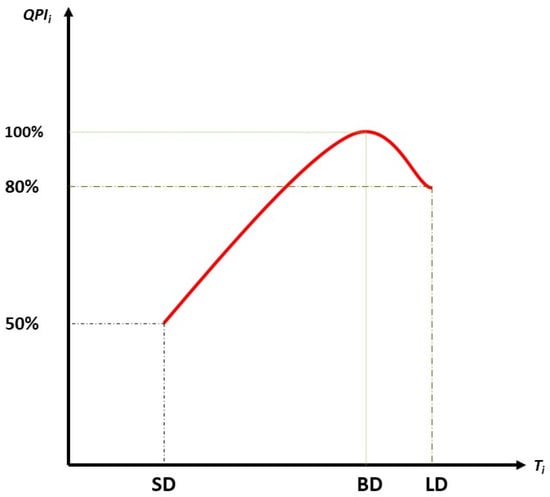
Figure 1. Quality performance index (QPI).

However, some resources might have a negative impact on the environment during the development phase of a project by generating CO₂. CO₂ emissions can occur in two ways during the on-site construction process: directly from electricity consumption and fuel combustion, and indirectly from the manufacturing of building materials and their transportation. CO₂ emissions can be reduced by not only selecting environmentally friendly materials, but also by ensuring that materials are transported in the shortest possible manner. Thus, the objective function to minimize the total amount of CO₂ in the project can be calculated by Equation (9).

$$\min \mathrm{CE}={\displaystyle \sum }_{\mathrm{i}=1}^{\mathrm{M}}{\mathrm{E}}_{\mathrm{dij}}+{\displaystyle \sum }_{\mathrm{i}=1}^{\mathrm{M}}{\mathrm{E}}_{\mathrm{inij}}=({\displaystyle \sum }_{\mathrm{i}=1}^{\mathrm{M}}{\mathrm{Q}}_{\mathrm{ed}}\times {\mathrm{F}}_{\mathrm{e}}+{\mathrm{Q}}_{\mathrm{dd}}\times {\mathrm{F}}_{\mathrm{d}})+({\displaystyle \sum }_{\mathrm{i}=1}^{\mathrm{M}}{\mathrm{Q}}_{\mathrm{k}}\times {\mathrm{F}}_{\mathrm{j}}+{\mathrm{Q}}_{\mathrm{ek}}\times {\mathrm{F}}_{\mathrm{e}}+{\mathrm{Q}}_{\mathrm{dk}}\times {\mathrm{F}}_{\mathrm{d}})$$

(9)

where $\mathrm{CE}$ is the total CO₂ emission in the project; ${\mathrm{E}}_{\mathrm{dij}}$ and ${\mathrm{E}}_{\mathrm{inij}}$ are the direct and indirect CO₂ emissions in the project, respectively; ${\mathrm{Q}}_{\mathrm{ed}}$ shows an activity’s electricity consumption; ${\mathrm{Q}}_{\mathrm{dd}}$ elucidates an activity’s diesel consumption; ${\mathrm{Q}}_{\mathrm{ij}}$ shows the consumption of material k in an activity; ${\mathrm{Q}}_{\mathrm{ek}}$ indicates the electricity consumption for the transportation of material k for an activity; ${\mathrm{Q}}_{\mathrm{dk}}$ shows the diesel consumption for the transportation of material k for an activity; ${\mathrm{F}}_{\mathrm{e}}$, ${\mathrm{F}}_{\mathrm{d}}$, and ${\mathrm{F}}_{\mathrm{j}}$ are the carbon emission factor (CEF) per electricity unit, diesel unit consumption, and per unit production of material k, respectively. Concerning the project’s risk, the actual project risk is mostly determined by the project’s circumstances, delivery systems, and contract terms. A “risk value” is described as a function that combines the two components: (i) the project’s overall float, and (ii) resource volatility. When noncritical operations have a high degree of temporal uncertainty, the usage of float may result in increased project risk and schedule overruns. Thus, construction managers are required to execute schedule adjustments to minimize unplanned changes in resource use throughout the duration of the project’s execution. Allowing noncritical operations to float may result in more effective resource use [79,80,81]. Consequently, the fifth objective function for risk can be formulated as Equation (10):

$$\min \mathrm{R}={\mathrm{w}}_1\times \left(1-\frac{{\mathrm{TF}}_{\mathrm{c}}+1}{{\mathrm{TF}}_{\max }+1}\right)+{\mathrm{w}}_2\times \left(\frac{{{\displaystyle \sum }}_{\mathrm{i}=1}^{\mathrm{Pd}}{\left({\mathrm{R}}_{\mathrm{t}}-\overline{\mathrm{R}}\right)}^2}{{\mathrm{P}}_{\mathrm{d}}{\left(\overline{\mathrm{R}}\right)}^2}\right)+{\mathrm{w}}_3\times \left(1-\frac{\stackrel{-}{\mathrm{R}}}{\max \left({\mathrm{R}}_{\mathrm{t}}\right)}\right)$$

(10)

where ${\mathrm{TF}}_{\mathrm{c}}$ and ${\mathrm{TF}}_{\max }$ show the total current float and total flexible scheduling float of the project; $\overline{\mathrm{R}}$ elucidates the uniform resource level; ${\mathrm{R}}_{\mathrm{t}}$ represents the resources required on day t; and w_i represents the weights.

Finally, to assess the capability of the FHO algorithm for the time–cost–quality–risk–CO₂ (All) trade-off, simultaneously, Equation (11) is used:

$$\mathrm{F}\left(\mathrm{x}\right)=\frac{\mathrm{T}-{\mathrm{T}}_{\min }}{{\mathrm{T}}_{\max }-{\mathrm{T}}_{\min }}+\frac{\mathrm{C}-{\mathrm{C}}_{\min }}{{\mathrm{C}}_{\max }-{\mathrm{C}}_{\min }}+\frac{\mathrm{R}-{\mathrm{R}}_{\min }}{{\mathrm{R}}_{\max }-{\mathrm{R}}_{\min }}+\frac{{\mathrm{CO}}_2-{\mathrm{CO}}_{2\left(\min \right)}}{{\mathrm{CO}}_{2\left(\max \right)}-{\mathrm{CO}}_{2\left(\min \right)}}+\frac{{\mathrm{Q}}_{\min }-\mathrm{Q}}{{\mathrm{Q}}_{\max }-{\mathrm{Q}}_{\min }}$$

(11)

3.2. BIM Module

A numerical case study is deemed to elucidate the efficiency of the FHO optimization algorithms in dealing with TCT problems. The case study is a five-floor residential building and a basement with a total floor area of 930 m² that is used to validate the FHO algorithm with five objectives: time, cost, quality, risk, and CO₂ emissions. As shown in Table A1, all activity information is elicited by the BIM process, project data, and experts’ judgments in the planning and designing steps. In other words, in completing this table, the experiences of various elite people and experts in this field have been used. The time and cost of executive mode NO.1 are the actual time and cost of the project extracted from the final status of the construction, NO.3 are obtained from BIM, and NO.5 are the contractor’s initial offers. In addition, two other executive modes were considered based on expert opinions in this field. Admittedly, contractors’ initial offers are often illogical and dreamy to attract the attention of employers, which is why most projects fail. Because most contractors do not consider rework, clashes, non-payment by employers, severe weather conditions, etc.; however, each activity is randomly written with three types of quality indicators at distinct percentages. The final quality in each line is obtained from the percentage of the total effects of those three quality modes. Finally, for each activity, the risk percentage is randomly deemed based on the viewpoints of elite professors and experts in this field.

The activity logic is finish to start for all activities. For modelling, the building was modelled in three different disciplines, including architecture, structure, mechanical, electrical, and pipeline (MEP) with Autodesk Revit 2022; meanwhile, all elements were modelled with Level of Development (LOD) 350 based on BIMFourm 2019 specifications. Subsequently, dynamo visual programming was used to generate parametric modelling in Revit. In the following stage, Navisworks software was employed for the project’s soft and hard clash detection. Finally, MATLAB is used for programming and trade-off of objective functions. The BIM model in the case study is shown in Figure 2.

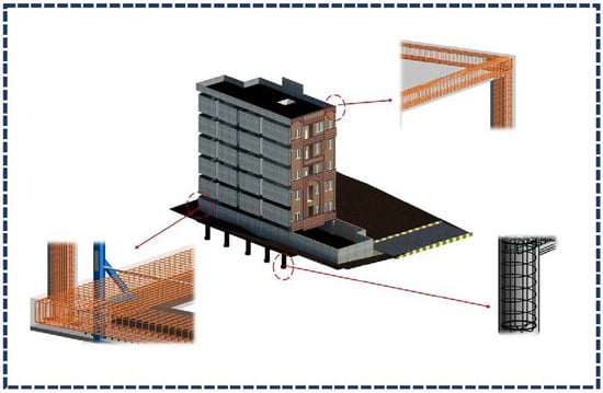
Figure 2. The project BIM-based modelling for resource trade-off.

3.3. Fire Hawk Optimizer (FHO)

3.3.1. Inspiration

Native Australians have long used fire to manage and preserve the balance of the surrounding ecology and terrain, and it has been a part of their cultural and ethnic traditions. People and other factors may spread intentionally started or naturally occurring fires caused by lightning, escalating the vulnerability of the native ecosystem and biodiversity. Furthermore, it was recently determined that black kites, whistling kites, and brown falcons are able to cause spreading fires throughout the region. The mentioned birds, known as Fire Hawks, strive to spread fire on purpose by carrying blazing sticks in their beaks and talons, a behaviour characterized as a natural catastrophe. The birds pick up burning sticks and deposit them in other unburned spots to make small fires to control and capture their prey. These small flames frighten their prey, such as snakes, rodents, and other animals, causing them to escape in a fast and panicked manner, making it much simpler for the hawks to capture them.

3.3.2. Mathematical Model

The FHO algorithm imitates the fire hawks’ foraging behaviour, taking into consideration the procedure of starting and spreading flames, as well as capturing prey. Initially, a set of possible solutions (X) are determined based on the fire hawks and prey’s position vectors. A random initialization mechanism is used to establish the initial positions of these vectors in the search space.

$$\mathrm{X}=\left[\begin{array}{c}{\mathrm{X}}_1\\ {\mathrm{X}}_2\\ ⋮\\ {\mathrm{X}}_{\mathrm{i}}\\ ⋮\\ {\mathrm{X}}_{\mathrm{N}}\end{array}\right]=\left[\begin{array}{c}{\mathrm{x}}_1^1 {\mathrm{x}}_1^2 \cdots {\mathrm{x}}_1^{\mathrm{j}} \cdots {\mathrm{x}}_1^{\mathrm{d}}\\ {\mathrm{x}}_2^1 {\mathrm{x}}_2^2 \cdots {\mathrm{x}}_2^{\mathrm{j}} \cdots {\mathrm{x}}_2^{\mathrm{d}}\\ ⋮ ⋮ ⋮ \ddots ⋮\\ {\mathrm{x}}_{\mathrm{i}}^1 {\mathrm{x}}_{\mathrm{i}}^2 \cdots {\mathrm{x}}_{\mathrm{i}}^{\mathrm{j}} \cdots {\mathrm{x}}_{\mathrm{i}}^{\mathrm{d}}\\ ⋮ ⋮ ⋮ \ddots ⋮\\ {\mathrm{x}}_{\mathrm{N}}^1 {\mathrm{x}}_{\mathrm{N}}^2 \cdots {\mathrm{x}}_{\mathrm{N}}^{\mathrm{j}} \cdots {\mathrm{x}}_{\mathrm{N}}^{\mathrm{d}}\end{array}\right],\{\begin{array}{c}\begin{array}{c}i=1,2,\dots ,\mathrm{N}.\end{array}\\ j=1,2,\dots ,\mathrm{d}.\end{array}$$

(12)

$${\mathrm{x}}_{\mathrm{i}}^{\mathrm{j}}\left(0\right)={\mathrm{x}}_{\mathrm{i},\min }^{\mathrm{j}}+\mathrm{rand}.\left({\mathrm{x}}_{\mathrm{i},\max }^{\mathrm{j}}-{\mathrm{x}}_{\mathrm{i},\min }^{\mathrm{j}}\right),\{\begin{array}{c}\begin{array}{c}i=1,2,\dots ,\mathrm{N}.\end{array}\\ j=1,2,\dots ,\mathrm{d}.\end{array}$$

(13)

where $\mathrm{N}$ elucidates the total number of solution candidates in the search space; ${\mathrm{X}}_{\mathrm{i}}$ shows the ith solution candidate in the search space;$\mathrm{d}$ is the considered problem’s dimension; ${\mathrm{x}}_{\mathrm{i}}^{\mathrm{j}}\left(0\right)$ represents the initial position of the solution candidates; ${\mathrm{x}}_{\mathrm{i}}^{\mathrm{j}}$ is the jth decision variable of the ith solution candidate; $\mathrm{rand}$ is a uniformly distributed random number in the range of (0, 1); and ${\mathrm{x}}_{\mathrm{i},\min }^{\mathrm{j}}$ and ${\mathrm{x}}_{\mathrm{i},\max }^{\mathrm{j}}$ are the minimum and maximum bounds of the jth decision variable for the ith solution candidate.

The specified optimization problem is taken into account during the objective function evaluation of solution candidates so as to identify the Fire Hawks in the search space. Predators and prey may be distinguished from one other by the greater objective function values of certain solution candidates. The selected Fire Hawks are employed to spread flames around the prey in the search zone, making hunting easier for the hunter. The main fire, which is originally employed by the Fire Hawks to spread flames over the search region, is also assumed to be the best global solution. These features are mathematically represented as follows:

$$\mathrm{PR}=\left[\begin{array}{c}{\mathrm{PR}}_1\\ {\mathrm{PR}}_2\\ ⋮\\ {\mathrm{PR}}_{\mathrm{k}}\\ ⋮\\ {\mathrm{PR}}_{\mathrm{m}}\end{array}\right],\mathrm{k}=1,2,\dots ,\mathrm{m}.$$

(14)

$$\mathrm{FH}=\left[\begin{array}{c}{\mathrm{FH}}_1\\ {\mathrm{FH}}_2\\ ⋮\\ {\mathrm{FH}}_{\mathrm{l}}\\ ⋮\\ {\mathrm{FH}}_{\mathrm{n}}\end{array}\right],\mathrm{l}=1,2,\dots ,\mathrm{n}.$$

(15)

where ${\mathrm{FH}}_{\mathrm{l}}$ explains the lth fire hawk in a complete search space of n fire hawks; and ${\mathrm{PR}}_{\mathrm{k}}$ reveals the kth prey in the search space depending the whole number of m preys.

The distance among the Fire Hawks and their prey is determined in the following step of the algorithm, where ${\mathrm{D}}_{\mathrm{k}}^{\mathrm{l}}$ is shown using the following equation:

$${\mathrm{D}}_{\mathrm{k}}^{\mathrm{l}}=\sqrt{{\left({\mathrm{x}}_2-{\mathrm{x}}_1\right)}^2+{\left({\mathrm{y}}_2-{\mathrm{y}}_1\right)}^2},\{\begin{array}{c}\mathrm{l}=1,2,\dots ,\mathrm{n}.\\ \mathrm{k}=1,2,\dots ,\mathrm{m}.\end{array}$$

(16)

where $\mathrm{m}$ and $\mathrm{n}$ demonstrate the overall number of preys and fire hawks in the search space, respectively; ${\mathrm{D}}_{\mathrm{k}}^{\mathrm{l}}$ shows the total distance between the lth fire hawk and the kth prey; and (${\mathrm{x}}_1,{\mathrm{y}}_1$) and (${\mathrm{x}}_2,{\mathrm{y}}_2$) represent the coordinates of the Fire Hawks and prey in the search space.

The territory of these birds is recognized using the nearest prey in the vicinity, using the method described above to determine the overall distance among Fire Hawks and prey.

After that, the Fire Hawks collect hot coals from the primary fire to start a fire at the designated spot. These two behaviours may be employed as location updating processes in FHO’s main search loop since some birds are willing to utilize burning sticks from other Fire Hawks’ territories, as illustrated in the equation below:

$${\mathrm{FH}}_{\mathrm{l}}^{\mathrm{new}}={\mathrm{FH}}_{\mathrm{l}}+\left({\mathrm{r}}_1\times \mathrm{GB}-{\mathrm{r}}_2\times {\mathrm{FH}}_{\mathrm{Near}}\right),\begin{array}{c}\mathrm{l}=1,2,\dots ,\mathrm{n}.\end{array}$$

(17)

where $\mathrm{GB}$ demonstrates the global best solution in the search space considered as the primary fire; ${\mathrm{FH}}_{\mathrm{l}}^{\mathrm{new}}$ shows the novel position vector of the lth Fire Hawk (${\mathrm{FH}}_{\mathrm{l}}$); and ${\mathrm{r}}_1$ and ${\mathrm{r}}_2$ are uniformly distributed random numbers in the range of (0, 1) for illustrating Fire Hawks’ movements towards the vital fire and the other Fire Hawks’ territories; and ${\mathrm{FH}}_{\mathrm{Near}}$ shows one of the Fire Hawks in the search space.

Prey movement throughout each fire informs the algorithm’s following stage, which involves updating positions, the hawk’s territory is seen as a crucial aspect of animal behaviour. The following equation could be employed to take these activities into account while updating a position:

$${\mathrm{PR}}_{\mathrm{q}}^{\mathrm{new}}={\mathrm{PR}}_{\mathrm{q}}+\left({\mathrm{r}}_3\times {\mathrm{FH}}_{\mathrm{l}}-{\mathrm{r}}_4\times {\mathrm{SP}}_{\mathrm{l}}\right),\{\begin{array}{c}\begin{array}{c}\mathrm{l}=1,2,\dots ,\mathrm{n}.\end{array}\\ \mathrm{q}=1,2,\dots ,\mathrm{r}.\end{array}$$

(18)

where $\mathrm{GB}$ is the global best solution in the search space considered as the main fire; ${\mathrm{PR}}_{\mathrm{q}}^{\mathrm{new}}$ is the novel position vector of the qth prey (${\mathrm{PR}}_{\mathrm{q}}$) surrounded by the lth Fire Hawk (${\mathrm{FH}}_{\mathrm{l}}$); ${\mathrm{SP}}_{\mathrm{l}}$ is a safe place under the lth Fire Hawk territory; and to ascertain the motions of prey in the direction of the Fire Hawks and the safe location, ${\mathrm{r}}_3$ and ${\mathrm{r}}_4$ are uniformly distributed random integers in the range of (0, 1).

Furthermore, the prey may move into the territory of other Fire Hawks. At the same time, there is a chance that the prey may approach the Fire Hawks that are trapped by neighbouring flames. Fire Hawks may even try to hide in a more secure region beyond the Fire Hawk’s territory. The following equation could be employed to account for these activities throughout the position updating process:

$${\mathrm{PR}}_{\mathrm{q}}^{\mathrm{new}}={\mathrm{PR}}_{\mathrm{q}}+\left({\mathrm{r}}_5\times {\mathrm{FH}}_{\mathrm{Alter}}-{\mathrm{r}}_6\times \mathrm{SP}\right),\{\begin{array}{c}\begin{array}{c}\mathrm{l}=1,2,\dots ,\mathrm{n}.\end{array}\\ \mathrm{q}=1,2,\dots ,\mathrm{r}.\end{array}$$

(19)

where ${\mathrm{PR}}_{\mathrm{q}}^{\mathrm{new}}$ shows the new position vector of the qth prey (${\mathrm{PR}}_{\mathrm{q}}$) flanked by the lth fire hawk (${\mathrm{FH}}_{\mathrm{l}}$); $\mathrm{SP}$ elucidates a safe place outside the lth Fire Hawk’s territory; ${\mathrm{FH}}_{\mathrm{Alter}}$ is one of the fire hawks in the search space; ${\mathrm{r}}_5$ and ${\mathrm{r}}_6$ indicate uniformly distributed random numbers in the range of (0, 1) to determine the movements of preys towards the other Fire Hawks and the safe region outside the territory.

The mathematical presentation of ${\mathrm{SP}}_{\mathrm{l}}$ and $\mathrm{SP}$ is stated as follows, taking into account the fact that the safe place in nature is a location where the majority of animals assemble so as to be safe and sound during a hazard:

$${\mathrm{SP}}_{\mathrm{l}}=\frac{{{\displaystyle \sum }}_{\mathrm{q}=1}^{\mathrm{r}}{\mathrm{PR}}_{\mathrm{q}}}{\mathrm{r}},\{\begin{array}{c}\mathrm{q}=1,2,\dots ,\mathrm{r}.\\ \mathrm{l}=1,2,\dots ,\mathrm{n}.\end{array}$$

(20)

$$\mathrm{SP}=\frac{{{\displaystyle \sum }}_{\mathrm{k}=1}^{\mathrm{m}}{\mathrm{PR}}_{\mathrm{k}}}{\mathrm{m}},\mathrm{k}=1,2,\dots ,\mathrm{m}.$$

(21)

where ${\mathrm{PR}}_{\mathrm{q}}$ shows the qth prey surrounded by the lth fire hawk (${\mathrm{FH}}_{\mathrm{l}}$); ${\mathrm{PR}}_{\mathrm{k}}$ is the kth prey in the search space.

The FHO algorithm’s pseudo-code is shown in Figure 3.

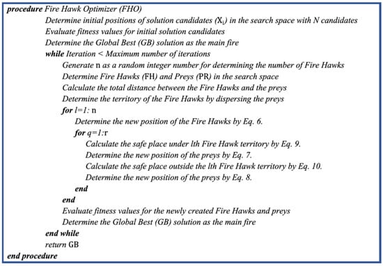
Figure 3. Pseudo-code of FHO.

4. Optimization Results

Five different metaheuristic algorithms were chosen to compare the efficacy of the FHO algorithm in solving resource trade-off problems in construction projects, including Firefly Algorithm (FA) [82], Multi-Verse Optimizer (MVO) [83], Particle Swarm Optimization (PSO) [84], Symbiotic Organisms Search (SOS) algorithm [85], and Teaching-learning-based Optimization (TLBO) [86]. All optimization processes have been conducted via MATLAB programming software using a PC with 8 GM RAM, CORE i7, and 2.8 GHz frequency. Table 2 shows the best findings of the FHO alongside other alternative algorithms for each scenario. However, for statistical purposes, 30 independent optimization runs are carried out for determining the statistical measurements as the mean, worst, standard deviation, and computational time. A predefined stopping criterion is also considered based on a maximum number of 5000 objective function evaluations, while the number of populations for each algorithm is determined by the maximum number of objective function evaluations and the maximum number of iterations. Figure 4 illustrates the convergence history of FHO and alternative algorithms in dealing with the mentioned trade-off problems.

Table 2. The best outcomes of the FHO and alternative algorithms for the case study.

	FA	MVO	PSO	SOS	TLBO	FHO (Current Study)
Time	261	258	321	258	281	258
Cost	118,230	117,056	119,564.8	117,104.6	117,512	116,783
Quality	94.35	94.16	93.82	94.41	93.89	87.81
Risk	5.78	5.94	6.53	5.78	5.93	5.78
CO2	76.35	76.74	103.35	76.35	79.60	76.35
All	0.74	0.76	0.99	0.74	0.77	0.74

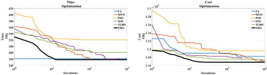
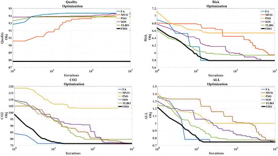
Figure 4. Convergence history of 30 independent optimization runs of FHO and alternative algorithms.

Table 3 demonstrates the statistical results of optimization in the case study. As can be seen, the FHO algorithm could dominate most of the alternative metaheuristic algorithms in the first scenario of time optimization in the case study, which calculates 258 days as the best and optimum time, similar to the MVO and SOS algorithms. Regarding standard deviation (Std), the FA algorithm delivers the most minimal result, followed by the FHO algorithm, accounting for 0.18. In comparison, the PSO algorithm provides the most significant value of Std, registered at about 35.07. Moreover, the SOS algorithm could conduct the time optimization process in the smallest feasible time (1.40 s); on the other hand, the longest computing time is acquired by the FHO and PSO algorithms, needing significantly more time to conduct the optimization process in this case. Evident is the fact that the FHO algorithm outperforms other alternative metaheuristic algorithms in the case study’s second scenario (cost optimization); in other words, the FHO algorithm can compute the project’s lowest cost, in contrast to the PSO algorithm’s maximum optimal value of cost. However, the FHO algorithm took the most computational time in this case, followed by the FA; conversely, the SOS algorithm took the least computing time for cost optimization in the project mentioned above. Additionally, the FHO algorithm supplied the smallest feasible Std value, followed by the FA. Meanwhile, the PSO achieved the greatest standard deviation of all algorithms studied in this case. Therefore, the FHO algorithm could be an acceptable metaheuristic for project and construction management cost optimization.

Table 3. The statistical outcomes of the algorithms.

	FA	MVO	PSO	SOS	TLBO	FHO (Current Study)
Time
Best	261	258	321	258	281	258
Mean	261	258.9	392.7	260.76	300.6	258.03
Worst	261	261	453	266	316	259
Std	0	1.21	35.07	1.71	9.04	0.18
Computational time (s)	2.19	1.61	2.35	1.40	1.44	8.66
Cost
Best	118,230	117,056	119,564.8	117,104.6	117,512	116,783
Mean	118,558.6	117,511.9	135,480.6	117,498.3	118,322.9	116,839.7
Worst	118,780	118,284.6	155,151.7	117,920	119,070	117,011
Std	148.09	271.58	9952.33	222.75	397.19	59.57
Computational time (s)	2.16	1.57	2.13	1.39	1.44	9.66
Quality
Best	94.35	94.16	93.82	94.41	93.89	87.81
Mean	94.46	94.24	93.89	94.54	94.01	89.63
Worst	94.56	94.40	94.12	94.62	94.27	91.46
Std	0.04	0.05	0.06	0.04	0.08	0.78
Computational time (s)	9.05	1.44	2.11	1.40	1.44	2.03
Risk
Best	5.78	5.94	6.53	5.78	5.93	5.78
Mean	5.78	6.07	7.13	5.79	6.03	5.78
Worst	5.78	6.28	7.46	5.82	6.20	5.78
Std	9.03 × 10−16	8.45 × 10−02	2.47 × 10−1	0.01	6.99 × 10−2	9.03 × 10−16
Computational time (s)	2.27	1.56	2.05	1.39	1.43	8.67
CO2
Best	76.35	76.44	103.35	76.35	79.60	76.35
Mean	76.35	77.87	116.23	76.68	88.24	76.40
Worst	76.35	80.41	129.54	77.20	94.47	76.59
Std	1.45 × 10−14	0.92	6.20	0.24	4.19	0.06
Computational time (s)	1.93	1.59	2.29	1.38	1.42	12.52
All
Best	0.74	0.76	0.99	0.74	0.77	0.74
Mean	0.74	0.84	1.42	0.75	0.86	0.74
Worst	0.74	0.95	1.67	0.78	0.94	0.74
Std	2.26 × 10−16	0.04	0.21	0.01	0.04	2.26 × 10−16
Computational time (s)	1.98	1.70	2.42	1.38	1.43	10.96

The statistical outcomes of the case study’s quality optimization indicate that the FHO method can deliver acceptable quality. Additionally, the SOS algorithm achieved the most outstanding quality value, about 94.41, followed by the FA algorithm. Additionally, the SOS algorithm could provide the smallest standard deviation, in this case, roughly 0.04. In sharp contrast, the FHO set the highest standard. However, in terms of computing time for quality optimization, in this case, the SOS algorithm required the least time, contrasted to the FHO approach, which required around 0.78 s. As a consequence, although the FHO algorithm can provide an acceptable level of quality, the SOS method could be a preferred choice for project managers in this circumstance. Nonetheless, similar to the FA and SOS algorithms, the FHO could calculate the lowest value for risk in the case study, accounting for nearly 5.78. Furthermore, the SOS algorithm required as little computational time as possible in this scenario, followed by the TLBO algorithm. Hence, the FHO algorithm could be a well-suited algorithm for risk optimization in project scheduling. Meanwhile, the FHO algorithm could calculate the lowest value for Std in this scenario.

Considering sustainability in construction, the FHO could be an ideal algorithm for project engineers to reduce the carbon footprint, since it could calculate the lowest CO₂ in the case study, thereby realizing environmentally friendly construction. In contrast, the PSO algorithm provided the highest value for CO₂ in this scenario, indicating its unfavorable performance in achieving the project with the lowest carbon footprint. However, the SOS algorithm gave the lowest computational time, registered at 1.38 (s), followed by TLBO. As a result, considering the average computational time, the FHO algorithm could be considered an appropriate alternative to optimize the amount of carbon dioxide in construction projects.

The FHO algorithm could outperform other metaheuristic algorithms in dealing with the TCQRCT problem by considering a residential dwelling as a case study, followed by the FA and SOS algorithms. Regarding Std. value, the FHO and FA algorithms gave the lowest value, indicating its superior performance. However, the SOS algorithm required the lowest computational time to conduct TCQRCT in the case study, followed by the TLBO, with nearly 1.43 (s). The FHO algorithm could be unique for TCQRCT problems in construction projects without considering computational time.

5. Discussion

The results and comparisons revealed that the FHO algorithm could outperform for some optimization problems in the studied case study; hence, the project managers should use this optimization process in their organizations or projects to obtain the most optimum solutions regarding time, cost, quality, risk, and CO₂.

The modes of all activities are shown in Table 4. It is clear that for the time optimization in the case study, all the mentioned algorithms opted for the third mode (BIM) as the BIM process was able to provide the optimum and best time for this residential building. Furthermore, regarding the cost, the first and second modes are preferable, followed by the third mode (BIM). Regarding the quality, almost all algorithms preferred the second mode, which is between the actual and the BIM. Undoubtedly, the first mode is the most preferable mode for all mentioned algorithms, indicating the proper mode for providing the optimum risk in the case study. Regarding the CO₂ and the All optimizations, the third mode is superior to the others. Meanwhile, it should be noted that the 4th and 5th modes were not preferred by any algorithms for any of the problems in the current case.

Table 4. Modes of different activities in optimization process.

Number	Objective	Mode of Activities
1	Time	FA:55555555555555555555555555555555555555
		MVO:55555555555555555555555555535555555555
		PSO:54435325555255525554445513453113245445
		SOS:55555555555555555555555555535555555555
		TLBO:55555555451455444555452455535554533555
		FHO:55555555555555555555555555535555555555
2	Cost	FA:43334343343242333433343332332343434342
		MVO:44423244423333243443442432432432444332
		PSO:23323225253434543344542434433424342234
		SOS:43423432334442343442432533432432434332
		TLBO:43444442424243244342432443234444244332
		FHO:43424442444242343442432442432442434332
3	Quality	FA:33331133333111131131333333331331133311
		MVO:13331131311313331331131111333133113311
		PSO:11111111111111111111111111111111111111
		SOS:13113333131333313313113333313313313133
		TLBO:11311111111111111111111113311111111111
		FHO:15344214411545354222554535254442254422
4	Risk	FA:22222222222222222222222222222222222222
		MVO:22222222222225525232222222222222252222
		PSO:22334322222225253225425431323232412424
		SOS:22222222222222222222222222222222222222
		TLBO:23222322322222222232231222222322222222
		FHO:22222222222222222222222222222222222222
5	CO2	FA:44444444444444444444444444444444444444
		MVO:15544232142225444342331444434454444444
		PSO:15544232142225444342331444434454444444
		SOS:44444444444444444444444444444444444444
		TLBO:54443454444543444544444445445444544444
		FHO:44444444444444444444444444444444444444
6	All	FA:33333333333333333333333333333333333333
		MVO:33333333333333323333333333333333333353
		PSO:33323343223244133333535234333222333333
		SOS:33333333333333333333333333333333333333
		TLBO:33333333333333333333333332333333332333
		FHO:33333333333333333333333333333333333333

Notably, there have been several instances in the construction industry when bad project management caused things to spiral out of control. The newest Veterans Affairs medical facility was supposed to have been built in Colorado by 2013, with a projected project cost of $328 million, according to a news report. However, the actual cost, which was $1.73 billion, went above budget by more than $1 billion. Additionally, the project took 5 years longer to finish than expected. This illustration demonstrates the seriousness with which optimization procedures and practical project management techniques, such as BIM, in construction should be approached [87]. Considering the current case study, the BIM process and the FHO algorithm could decrease the total cost from approximately $125,630 to nearly $116,839.70, a 7% reduction in cost. Therefore, implementing the BIM process in large-scale projects such as the Veterans Affairs medical facility could save $121 million. Furthermore, since BIM and the FHO algorithm could diminish the total time from 313 to 258 days (17.5%), they could decrease the total time of the project’s execution, thereby decreasing the indirect and direct costs, as well as the CO₂ emission caused by the logistics and equipment at the project’s site. Furthermore, project managers and schedulers of all projects are able to analyze and propose the most feasible resource options, considering the organization’s goals and scopes, to the employers or owners by using the BIM process and an optimization process with metaheuristic algorithms, such as the FHO algorithm.

6. Conclusions

This paper established a unique framework that involves building information modelling (BIM) and a novel metaheuristic algorithm to solve the resources trade-off problem in construction projects. For this purpose, Fire Hawk Optimizer (FHO) is used as a novel metaheuristic algorithm. A 3D BIM-based modelling of the case study was created using different software, including Revit, Navisworks, Lumion, and also dynamo was utilized to perform parametric modelling. The key results and main outcomes of this research work are summarized as follows:

• Based on the outcomes of best optimization runs conducted by different methods in dealing with time optimization, the FHO algorithm could reach the lowest time for the case study, accounting for 258 days.
• The FHO can provide 116,783 ($) for the cost of the case study, which is the best among all approaches.
• Regarding quality optimization, the FHO is capable of providing reasonable quality value, but the SOS algorithm gave the best results.
• The FHO algorithm is able to provide the best results for both risk and CO₂ optimization in the case study, compared to other alternative algorithms.
• Based on the best results of the TCQRCT problem, the FHO algorithm can provide a score of 0.74, which is much better than the other algorithms.

Based on the results and conducted analysis, the main reasons for the superiority of the FHO algorithm compared to the other mentioned metaheuristics algorithms are threefold; namely, fast convergence behavior, being parameter-free, and the lowest possible objective function evaluation. The limitation of this research work is that only a residential building was used as the case study, and thus, future works should evaluate the capability of the FHO algorithm for other case studies, such as residential projects or infrastructure construction projects, and compare the results with those of other metaheuristic algorithms. Furthermore, the FHO algorithm should be tested for future studies utilizing intricate optimization problems in miscellaneous fields, such as real-size engineering design problems such as truss structures. Additionally, future works should focus on proposing and developing the multi-objective version of the FHO algorithm (MOFHO) in order to optimize the time, cost, quality, risk, and CO₂ in a two-by-two manner.

References

- Feng, C.-W.; Liu, L.; Burns, S.A. Using Genetic Algorithms to Solve Construction Time-Cost Trade-Off Problems. J. Comput. Civ. Eng. 1997, 11, 184–189. [Google Scholar] [CrossRef]
- Chen, P.-H.; Weng, H. A two-phase GA model for resource-constrained project scheduling. Autom. Constr. 2009, 18, 485–498. [Google Scholar] [CrossRef]
- Tran, D.H.; Long, L.D. Project scheduling with time, cost and risk trade-off using adaptive multiple objective differential evolution. Eng. Constr. Archit. Manag. 2018, 25, 623–638. [Google Scholar] [CrossRef]
- Orm, M.B.; Jeunet, J. Time cost quality trade-off problems: A survey exploring the assessment of quality. Comput. Ind. Eng. 2018, 118, 319–328. [Google Scholar] [CrossRef]
- Shankar, N.R.; Raju, M.; Srikanth, G.; Bindu, P.H. Time, cost and quality trade-off analysis in construction of projects. Contemp. Eng. Sci. 2011, 4, 289–299. [Google Scholar]
- Lotfi, R.; Yadegari, Z.; Hosseini, S.; Khameneh, A.; Tirkolaee, E.; Weber, G. A robust time-cost-quality-energy-environment trade-off with resource-constrained in project management: A case study for a bridge construction project. J. Ind. Manag. Optim. 2022, 18, 375–396. [Google Scholar] [CrossRef]
- Monghasemi, S.; Nikoo, M.R.; Fasaee, M.A.K.; Adamowski, J. A novel multi criteria decision making model for optimizing time–cost–quality trade-off problems in construction projects. Expert Syst. Appl. 2015, 42, 3089–3104. [Google Scholar] [CrossRef]
- Abbasi, S.; Noorzai, E. The BIM-Based multi-optimization approach in order to determine the trade-off between embodied and operation energy focused on renewable energy use. J. Clean. Prod. 2021, 281, 125359. [Google Scholar] [CrossRef]
- Nguyen, D.-T.; Chou, J.-S.; Tran, D.-H. Integrating a novel multiple-objective FBI with BIM to determine tradeoff among resources in project scheduling. Knowl.-Based Syst. 2022, 235, 107640. [Google Scholar] [CrossRef]
- Dhiman, G.; Garg, M.; Nagar, A.; Kumar, V.; Dehghani, M. A novel algorithm for global optimization: Rat Swarm Optimizer. J. Ambient Intell. Humaniz. Comput. 2021, 12, 8457–8482. [Google Scholar] [CrossRef]
- Yampolskiy, R.V.; Ashby, L.; Hassan, L. Wisdom of Artificial Crowds—A Metaheuristic Algorithm for Optimization. J. Intell. Learn. Syst. Appl. 2012, 4, 98–107. [Google Scholar] [CrossRef]
- Xie, L.; Han, T.; Zhou, H.; Zhang, Z.-R.; Han, B.; Tang, A. Tuna Swarm Optimization: A Novel Swarm-Based Metaheuristic Algorithm for Global Optimization. Comput. Intell. Neurosci. 2021, 2021, 9210050. [Google Scholar] [CrossRef] [PubMed]
- Karaboga, D.; Basturk, B. Artificial bee colony (ABC) optimization algorithm for solving constrained optimization problems. In Proceedings of the Foundations of Fuzzy Logic and Soft Computing, Berlin/Heidelberg, Germany, 18–21 June 2007; pp. 789–798. [Google Scholar]
- Talatahari, S.; Azizi, M.; Gandomi, A.H. Material Generation Algorithm: A Novel Metaheuristic Algorithm for Optimization of Engineering Problems. Processes 2021, 9, 859. [Google Scholar] [CrossRef]
- Azizi, M.; Shishehgarkhaneh, M.B.; Basiri, M. Optimum design of truss structures by Material Generation Algorithm with discrete variables. Decis. Anal. J. 2022, 3, 100043. [Google Scholar] [CrossRef]
- Azizi, M. Atomic orbital search: A novel metaheuristic algorithm. Appl. Math. Model. 2021, 93, 657–683. [Google Scholar] [CrossRef]
- Azizi, M.; Talatahari, S.; Giaralis, A. Optimization of Engineering Design Problems Using Atomic Orbital Search Algorithm. IEEE Access 2021, 9, 102497–102519. [Google Scholar] [CrossRef]
- Azizi, M.; Mohamed, A.W.; Shishehgarkhaneh, M.B. Optimum design of truss structures with atomic orbital search considering discrete design variables. In Handbook of Nature-Inspired Optimization Algorithms: The State of the Art; Springer: Cham, Switzerland, 2022; pp. 189–214. [Google Scholar]
- Cunz, D.; Larson, D. Building information modeling. Under Constr. Am. Bar Assoc. 2006, 1–3. Available online: http://www.imageserve.com/naples2013/eunder_construction_12_06.pdf (accessed on 12 September 2022).
- Borrmann, A.; König, M.; Koch, C.; Beetz, J. Building Information Modeling: Technologische Grundlagen und Industrielle Praxis; Springer: Wiesbaden, Germany, 2015. [Google Scholar]
- Khondoker, M.T.H. Automated reinforcement trim waste optimization in RC frame structures using building information modeling and mixed-integer linear programming. Autom. Constr. 2021, 124, 103599. [Google Scholar] [CrossRef]
- Baghalzadeh Shishehgarkhaneh, M.; Fard Moradinia, S. The role of Building Information Modeling (BIM) in reducing the number of project dispute resolution sessions. In Proceedings of the 8th National Conference on Civil Engineering, Architecture and Sustainable Urban Development of Iran, Mashhad, Iran, 5 November 2020. [Google Scholar]
- Farzaneh, A.; Monfet, D.; Forgues, D. Review of using Building Information Modeling for building energy modeling during the design process. J. Build. Eng. 2019, 23, 127–135. [Google Scholar] [CrossRef]
- Charef, R.; Alaka, H.; Emmitt, S. Beyond the third dimension of BIM: A systematic review of literature and assessment of professional views. J. Build. Eng. 2018, 19, 242–257. [Google Scholar] [CrossRef]
- Charef, R.; Emmitt, S.; Alaka, H.; Fouchal, F. Building Information Modelling adoption in the European Union: An overview. J. Build. Eng. 2019, 25, 100777. [Google Scholar] [CrossRef]
- Seyis, S. Mixed method review for integrating building information modeling and life-cycle assessments. Build. Environ. 2020, 173, 106703. [Google Scholar] [CrossRef]
- Daqiqnia, A.H.; Fard Moradinia, S.; Baghalzadeh Shishehgarkhaneh, M. Toward Nearly Zero Energy Building Designs: A Comparative Study of Various Techniques. AUT J. Civ. Eng. 2021, 5, 12. [Google Scholar]
- Nadeem, A.; Wong, A.K.D.; Wong, F.K.W. Bill of Quantities with 3D Views Using Building Information Modeling. Arab. J. Sci. Eng. 2015, 40, 2465–2477. [Google Scholar] [CrossRef]
- Van Eynde, R.; Vanhoucke, M. A reduction tree approach for the Discrete Time/Cost Trade-Off Problem. Comput. Oper. Res. 2022, 143, 105750. [Google Scholar] [CrossRef]
- Sonmez, R.; Bettemir, Ö.H. A hybrid genetic algorithm for the discrete time–cost trade-off problem. Expert Syst. Appl. 2012, 39, 11428–11434. [Google Scholar] [CrossRef]
- Babu, A.J.G.; Suresh, N. Project management with time, cost, and quality considerations. Eur. J. Oper. Res. 1996, 88, 320–327. [Google Scholar] [CrossRef]
- Khang, D.B.; Myint, Y.M. Time, cost and quality trade-off in project management: A case study. Int. J. Proj. Manag. 1999, 17, 249–256. [Google Scholar] [CrossRef]
- Ndamlabin Mboula, J.E.; Kamla, V.C.; Tayou Djamegni, C. Cost-time trade-off efficient workflow scheduling in cloud. Simul. Model. Pract. Theory 2020, 103, 102107. [Google Scholar] [CrossRef]
- Hu, W.; He, X. An Innovative Time-Cost-Quality Tradeoff Modeling of Building Construction Project Based on Resource Allocation. Sci. World J. 2014, 2014, 673248. [Google Scholar] [CrossRef]
- Afruzi, E.N.; Najafi, A.A.; Roghanian, E.; Mazinani, M. A multi-objective imperialist competitive algorithm for solving discrete time, cost and quality trade-off problems with mode-identity and resource-constrained situations. Comput. Oper. Res. 2014, 50, 80–96. [Google Scholar] [CrossRef]
- Sharma, K.; Trivedi, M.K. AHP and NSGA-II-Based time–cost–quality trade-off optimization model for construction projects. In Artificial Intelligence and Sustainable Computing, Proceedings of the 4th International Conference on Sustainable and Innovative Solutions for Current Challenges in Engineering & Technology, ICSISCET 2022, Gwalior, India, 18–19 December 2022; Springer: Singapore, 2022; pp. 45–63. [Google Scholar]
- Ozcan-Deniz, G.; Zhu, Y.; Ceron, V. Time, cost, and environmental impact analysis on construction operation optimization using genetic algorithms. J. Manag. Eng. 2012, 28, 265–272. [Google Scholar] [CrossRef]
- Tran, D.-H.; Luong-Duc, L.; Duong, M.-T.; Le, T.-N.; Pham, A.-D. Opposition multiple objective symbiotic organisms search (OMOSOS) for time, cost, quality and work continuity tradeoff in repetitive projects. J. Comput. Des. Eng. 2018, 5, 160–172. [Google Scholar] [CrossRef]
- Luong, D.-L.; Tran, D.-H.; Nguyen, P.T. Optimizing multi-mode time-cost-quality trade-off of construction project using opposition multiple objective difference evolution. Int. J. Constr. Manag. 2021, 21, 271–283. [Google Scholar] [CrossRef]
- Mohammadipour, F.; Sadjadi, S.J. Project cost–quality–risk tradeoff analysis in a time-constrained problem. Comput. Ind. Eng. 2016, 95, 111–121. [Google Scholar] [CrossRef]
- Amoozad Mahdiraji, H.; Sedigh, M.; Razavi Hajiagha, S.H.; Garza-Reyes, J.A.; Jafari-Sadeghi, V.; Dana, L.-P. A novel time, cost, quality and risk tradeoff model with a knowledge-based hesitant fuzzy information: An R&D project application. Technol. Forecast. Soc. Chang. 2021, 172, 121068. [Google Scholar] [CrossRef]
- Sharma, K.; Trivedi, M.K. Latin hypercube sampling-based NSGA-III optimization model for multimode resource constrained time–cost–quality–safety trade-off in construction projects. Int. J. Constr. Manag. 2020, 1–11. [Google Scholar] [CrossRef]
- Keshavarz, E.; Shoul, A. Project Time-Cost-Quality Trade-off Problem: A Novel Approach Based on Fuzzy Decision Making. Int. J. Uncertain. Fuzziness Knowl.-Based Syst. 2020, 28, 545–567. [Google Scholar] [CrossRef]
- He, W.; Shi, Y.; Kong, D. Construction of a 5D duration and cost optimisation model based on genetic algorithm and BIM. J. Eng. Des. Technol. 2019, 17, 929–942. [Google Scholar] [CrossRef]
- Rahmani Asl, M.; Zarrinmehr, S.; Bergin, M.; Yan, W. BPOpt: A framework for BIM-based performance optimization. Energy Build. 2015, 108, 401–412. [Google Scholar] [CrossRef]
- Sekhar, A.; Maheswari, J.U. BIM integration and value engineering: Design for assembly, optimization, and real time cost visualization in off-site construction. In Proceedings of the Construction Research Congress 2022, Arlington, VA, USA, 9–12 March 2022; pp. 791–801. [Google Scholar]
- Kim, S.; Chin, S.; Kwon, S. A Discrepancy Analysis of BIM-Based Quantity Take-Off for Building Interior Components. J. Manag. Eng. 2019, 35, 05019001. [Google Scholar] [CrossRef]
- ElMenshawy, M.; Marzouk, M. Automated BIM schedule generation approach for solving time–cost trade-off problems. Eng. Constr. Archit. Manag. 2021, 28, 3346–3367. [Google Scholar] [CrossRef]
- Mashayekhi, A.; Heravi, G. A decision-making framework opted for smart building’s equipment based on energy consumption and cost trade-off using BIM and MIS. J. Build. Eng. 2020, 32, 101653. [Google Scholar] [CrossRef]
- Yongge, X.; Ya, W. Study on trade-off of time-cost-quality in construction project based on BIM. In Proceedings of the 2015 International Conference on Economics, Social Science, Arts, Education and Management Engineering, Xi’an, China, 12–13 December 2015; pp. 864–870. [Google Scholar]
- Yu, J.; Wang, J.; Hua, Z.; Wang, X. BIM-based time-cost optimization of a large-span spatial steel structure in an airport terminal building. J. Facil. Manag. 2021, 20, 469–484. [Google Scholar] [CrossRef]
- Gelisen, G.; Griffis, F.H. Automated Productivity-Based Schedule Animation: Simulation-Based Approach to Time-Cost Trade-Off Analysis. J. Constr. Eng. Manag. 2014, 140, B4013007. [Google Scholar] [CrossRef]
- Khosakitchalert, C.; Yabuki, N.; Fukuda, T. Improving the accuracy of BIM-based quantity takeoff for compound elements. Autom. Constr. 2019, 106, 102891. [Google Scholar] [CrossRef]
- Ma, G.; Zhang, L. Exact Overlap Rate Analysis and the Combination with 4D BIM of Time-Cost Tradeoff Problem in Project Scheduling. Adv. Civ. Eng. 2019, 2019, 9120795. [Google Scholar] [CrossRef]
- Shadram, F.; Mukkavaara, J. An integrated BIM-based framework for the optimization of the trade-off between embodied and operational energy. Energy Build. 2018, 158, 1189–1205. [Google Scholar] [CrossRef]
- Sandberg, M.; Mukkavaara, J.; Shadram, F.; Olofsson, T. Multidisciplinary Optimization of Life-Cycle Energy and Cost Using a BIM-Based Master Model. Sustainability 2019, 11, 286. [Google Scholar] [CrossRef]
- Baghalzadeh Shishehgarkhaneh, M.; Fard Moradinia, S.; Keivani, A. Time and cost management of dam construction projects based on Building Information Modeling (BIM) (A Case Study in Kurdistan Province). In Proceedings of the 7th International Congress on Civil Engineering, Architecture and Urban Development, Tehran, Iran, 7–9 December 2021. [Google Scholar]
- Azizi, M.; Talatahari, S.; Gandomi, A.H. Fire Hawk Optimizer: A novel metaheuristic algorithm. Artif. Intell. Rev. 2022. [Google Scholar] [CrossRef]
- Hajiagha, S.H.R.; Akrami, H.; Hashemi, S.S.; Mahdiraji, H.A. An integer grey goal programming for project time, cost and quality trade-off. Eng. Econ. 2015, 26, 93–100. [Google Scholar]
- Zheng, H. The bi-level optimization research for time-cost-quality-environment trade-off scheduling problem and its application to a construction project. In Proceedings of the Tenth International Conference on Management Science and Engineering Management, Baku, Azerbaijan, 30 August–2 September 2016; pp. 745–753. [Google Scholar]
- Al Haj, R.A.; El-Sayegh, S.M. Time–cost optimization model considering float-consumption impact. J. Constr. Eng. Manag. 2015, 141, 04015001. [Google Scholar] [CrossRef]
- Khalili-Damghani, K.; Tavana, M.; Abtahi, A.-R.; Santos Arteaga, F.J. Solving multi-mode time–cost–quality trade-off problems under generalized precedence relations. Optim. Methods Softw. 2015, 30, 965–1001. [Google Scholar] [CrossRef]
- Moghadam, E.K.; Sharifi, M.; Rafiee, S.; Chang, Y.K. Time–Cost–Quality Trade-Off in a Broiler Production Project Using Meta-Heuristic Algorithms: A Case Study. Agriculture 2019, 10, 3. [Google Scholar] [CrossRef]
- Zahraie, B.; Tavakolan, M. Stochastic time-cost-resource utilization optimization using nondominated sorting genetic algorithm and discrete fuzzy sets. J. Constr. Eng. Manag. 2009, 135, 1162–1171. [Google Scholar] [CrossRef]
- Huynh, V.-H.; Nguyen, T.-H.; Pham, H.C.; Huynh, T.-M.-D.; Nguyen, T.-C.; Tran, D.-H. Multiple Objective Social Group Optimization for Time–Cost–Quality–Carbon Dioxide in Generalized Construction Projects. Int. J. Civ. Eng. 2021, 19, 805–822. [Google Scholar] [CrossRef]
- Banihashemi, S.A.; Khalilzadeh, M. Time-cost-quality-environmental impact trade-off resource-constrained project scheduling problem with DEA approach. Eng. Constr. Archit. Manag. 2020, 28, 1979–2004. [Google Scholar] [CrossRef]
- Ghoddousi, P.; Eshtehardian, E.; Jooybanpour, S.; Javanmardi, A. Multi-mode resource-constrained discrete time–cost-resource optimization in project scheduling using non-dominated sorting genetic algorithm. Autom. Constr. 2013, 30, 216–227. [Google Scholar] [CrossRef]
- Mahmoudi, A.; Feylizadeh, M.R. A grey mathematical model for crashing of projects by considering time, cost, quality, risk and law of diminishing returns. Grey Syst. Theory Appl. 2018, 8, 272–294. [Google Scholar] [CrossRef]
- Ebrahimnezhad, S.; Ahmadi, V.; Javanshir, H. Time-cost-quality trade-off in a CPM1 network using fuzzy logic and genetic algorithm. Int. J. Ind. Eng. Prod. Manag. 2013, 24, 361–376. [Google Scholar]
- Mungle, S.; Benyoucef, L.; Son, Y.-J.; Tiwari, M. A fuzzy clustering-based genetic algorithm approach for time–cost–quality trade-off problems: A case study of highway construction project. Eng. Appl. Artif. Intell. 2013, 26, 1953–1966. [Google Scholar] [CrossRef]
- Koo, C.; Hong, T.; Kim, S. An integrated multi-objective optimization model for solving the construction time-cost trade-off problem. J. Civ. Eng. Manag. 2015, 21, 323–333. [Google Scholar] [CrossRef]
- Heravi, G.; Moridi, S. Resource-constrained time-cost tradeoff for repetitive construction projects. KSCE J. Civ. Eng. 2019, 23, 3265–3274. [Google Scholar] [CrossRef]
- Jeunet, J.; Bou Orm, M. Optimizing temporary work and overtime in the Time Cost Quality Trade-off Problem. Eur. J. Oper. Res. 2020, 284, 743–761. [Google Scholar] [CrossRef]
- Hamta, N.; Ehsanifar, M.; Sarikhani, J. Presenting a goal programming model in the time-cost-quality trade-off. Int. J. Constr. Manag. 2021, 21, 1–11. [Google Scholar] [CrossRef]
- Kosztyán, Z.T.; Szalkai, I. Hybrid time-quality-cost trade-off problems. Oper. Res. Perspect. 2018, 5, 306–318. [Google Scholar] [CrossRef]
- Azizi, M.; Mousavi, A.; Ejlali, R.; Talatahari, S. Optimum design of fuzzy controller using hybrid ant lion optimizer and Jaya algorithm. Artif. Intell. Rev. 2020, 53, 1553–1584. [Google Scholar] [CrossRef]
- Panwar, A.; Jha, K.N. Integrating Quality and Safety in Construction Scheduling Time-Cost Trade-Off Model. J. Constr. Eng. Manag. 2021, 147, 04020160. [Google Scholar] [CrossRef]
- Zhang, L.; Du, J.; Zhang, S. Solution to the time-cost-quality trade-off problem in construction projects based on immune genetic particle swarm optimization. J. Manag. Eng. 2014, 30, 163–172. [Google Scholar] [CrossRef]
- Al-Gahtani, K.S. Float Allocation Using the Total Risk Approach. J. Constr. Eng. Manag. 2009, 135, 88–95. [Google Scholar] [CrossRef]
- Garza, J.M.d.l.; Prateapusanond, A.; Ambani, N. Preallocation of Total Float in the Application of a Critical Path Method Based Construction Contract. J. Constr. Eng. Manag. 2007, 133, 836–845. [Google Scholar] [CrossRef]
- Long, L.D.; Tran, D.-H.; Nguyen, P.T. Hybrid multiple objective evolutionary algorithms for optimising multi-mode time, cost and risk trade-off problem. Int. J. Comput. Appl. Technol. 2019, 60, 203–214. [Google Scholar] [CrossRef]
- Yang, X.-S. Firefly algorithm, stochastic test functions and design optimisation. arXiv 2010, arXiv:1003.1409. [Google Scholar] [CrossRef]
- Mirjalili, S.; Mirjalili, S.; Hatamlou, A. Multi-Verse Optimizer: A nature-inspired algorithm for global optimization. Neural Comput. Appl. 2015, 27, 495–513. [Google Scholar] [CrossRef]
- Eberhart, R.; Kennedy, J. Particle swarm optimization. In Proceedings of the IEEE International Conference on Neural Networks, Perth, Australia, 27 November–1 December 1995; pp. 1942–1948. [Google Scholar]
- Tejani, G.G.; Savsani, V.J.; Patel, V.K. Adaptive symbiotic organisms search (SOS) algorithm for structural design optimization. J. Comput. Des. Eng. 2016, 3, 226–249. [Google Scholar] [CrossRef]
- Rao, R.V. Teaching-learning-based optimization algorithm. In Teaching Learning Based Optimization Algorithm; Springer: Cham, Switzerland, 2016; pp. 9–39. [Google Scholar]
- Gutierrez, G.; Gardella, R.; Ryan, B. New Colorado VA Hospital Is State of the Art, and More than $1 Billion Over Budget. Available online: https://www.nbcnews.com/storyline/va-hospital-scandal/new-colorado-va-hospital-state-art-more-1-billion-over-n898091 (accessed on 18 August 2020).
Publisher’s Note: MDPI stays neutral with regard to jurisdictional claims in published maps and institutional affiliations. |
© 2022 by the authors. Licensee MDPI, Basel, Switzerland. This article is an open access article distributed under the terms and conditions of the Creative Commons Attribution (CC BY) license (https://creativecommons.org/licenses/by/4.0/).