Article

On the Quantification of Visual Texture Complexity

by
Fereshteh Mirjalili
* and
Jon Yngve Hardeberg
Department of Computer Science, Norwegian University of Science and Technology (NTNU), 2815 Gjøvik, Norway
*
Author to whom correspondence should be addressed.
J. Imaging 2022, 8(9), 248; https://doi.org/10.3390/jimaging8090248
Submission received: 15 March 2022 / Revised: 26 August 2022 / Accepted: 8 September 2022 / Published: 10 September 2022
(This article belongs to the Special Issue Color Texture Classification)

Abstract

:
Complexity is one of the major attributes of the visual perception of texture. However, very little is known about how humans visually interpret texture complexity. A psychophysical experiment was conducted to visually quantify the seven texture attributes of a series of textile fabrics: complexity, color variation, randomness, strongness, regularity, repetitiveness, and homogeneity. It was found that the observers could discriminate between the textures with low and high complexity using some high-level visual cues such as randomness, color variation, strongness, etc. The results of principal component analysis (PCA) on the visual scores of the above attributes suggest that complexity and homogeneity could be essentially the underlying attributes of the same visual texture dimension, with complexity at the negative extreme and homogeneity at the positive extreme of this dimension. We chose to call this dimension visual texture complexity. Several texture measures including the first-order image statistics, co-occurrence matrix, local binary pattern, and Gabor features were computed for images of the textiles in sRGB, and four luminance-chrominance color spaces (i.e., HSV, YCbCr, Ohta’s I1I2I3, and CIELAB). The relationships between the visually quantified texture complexity of the textiles and the corresponding texture measures of the images were investigated. Analyzing the relationships showed that simple standard deviation of the image luminance channel had a strong correlation with the corresponding visual ratings of texture complexity in all five color spaces. Standard deviation of the energy of the image after convolving with an appropriate Gabor filter and entropy of the co-occurrence matrix, both computed for the image luminance channel, also showed high correlations with the visual data. In this comparison, sRGB, YCbCr, and HSV always outperformed the I1I2I3 and CIELAB color spaces. The highest correlations between the visual data and the corresponding image texture features in the luminance-chrominance color spaces were always obtained for the luminance channel of the images, and one of the two chrominance channels always performed better than the other. This result indicates that the arrangement of the image texture elements that impacts the observer’s perception of visual texture complexity cannot be represented properly by the chrominance channels. This must be carefully considered when choosing an image channel to quantify the visual texture complexity. Additionally, the good performance of the luminance channel in the five studied color spaces proves that variations in the luminance of the texture, or as one could call the luminance contrast, plays a crucial role in creating visual texture complexity.

1. Introduction

Visual complexity is a well-known concept in many disciplines including neuroscience [1,2], cognitive psychology [3,4,5], product marketing [6,7], web design [8,9], art [10], etc. From a theoretical point of view, studying visual complexity has revealed information about the human visual system operation when evaluating stimuli [2], the memory formation mechanism [1], and its capacity [11]. It has also helped psychologists to understand how the visual complexity of scenes impacts emotion and attracts attention [12]. From a practical perspective, research into visual complexity has aided the marketing industry in being able to better capture the consumer’s attention through pleasing and understandable advertisements [7]. It has also helped website designers to understand the influence of design features including complexity on the initial user impressions [9] and the cognitive effort a user needs to make to interact with web pages [8].
Visual complexity research has inevitably found its way into the domain of computer vision. The impact of complexity on the segmentation of histopathology images for the computer-aided diagnosis of cancer [13] and object detection in cluttered images [14,15] are two of the applications where visual complexity has played a critical role.
In the field of visual appearance, complexity might be naturally related to any of the appearance attributes, whether it be color, gloss, translucency, or texture, separately or in combination. For instance, spatio-chromatic complexity is associated with spatial and color variations on a surface that involves the perception of both color and texture at the same time [16]. The International Commission on Illumination (CIE) has assigned the technical committee “8–14: Specification of spatio-chromatic complexity” to devoting research on this visual phenomenon [17].
Research has provided significant evidence that humans are capable of perceiving and evaluating the complexity of scenes. A scene can be perceived as visually complex depending on the type and number of elements it contains and their spatial layout [18]. Various definitions for visual complexity have been proposed in the literature. The theory of complexity perception was introduced by Birkhoff [19] as an attempt to propose an aesthetic measure of an art object as the ratio between its order and complexity. He defined complexity as “a preliminary effort of attention, which is necessary for the act of perception”. In an attempt to prepare a standardized set of images for memory and cognitive processing research, Snodgrass and Vanderwart [20] found that familiarity and visual complexity are two independent attributes of a set of 260 line-drawn images. They defined visual complexity as “the amount of detail or intricacy” in the image. Heaps and Handel [21] defined visual complexity of the natural texture images as “how difficult it would be to give a verbal description of the texture”.
Complexity has been proven to be one of the main attributes of texture perception by several research works [22,23,24,25,26,27,28]. In one of the earliest studies on the visual properties of texture, Amadasun and King [22] introduced coarseness, contrast, busyness, complexity, and texture strength as the five properties of texture. They defined the texture complexity as the visual content of a texture, where the visual content referred to the patches or primitives, lines, and/or sharp edges present in the texture, having different intensities.
In an attempt to find the texture features that are important in texture perception, Rao and Lohse [23] asked twenty participants to perform an unsupervised classification of thirty pictures from Brodatz’s album [29], according to their similarity in texture. The results of multidimensional scaling analysis (MDS) indicated that perceptual texture can be characterized by the aid of only three features (i.e., repetition, orientation, and complexity). In a similar work, Mojsilovic et al. [24] performed a similarity analysis followed by multidimensional scaling (MDS) and hierarchical cluster analysis on a series of twenty color patterns from an interior design catalog. The main goal of the work was to find the basic dimensions of color patterns and their relationships. As a result, five categories that observers used to judge the similarity and matching of color patterns were found: overall color, directionality and orientation, regularity and placement, color purity, and complexity and heaviness. The fifth dimension, pattern complexity, and heaviness seemed to contain both the perceived color and luminance information.
Guo et al. [25] investigated the human Kansei of the complexity of visual scenes with a focus on texture perception. Kansei, a Japanese-origin word, is a technical term widely used in industrial design. Kansei engineering is a method of translating the consumer’s psychological needs and feelings for a product into design elements [30]. Through the verbal description of the texture of twenty images from Brodatz’s album and a subsequent factor analysis, they found that the major characteristics of texture that affect the human perception of visual complexity are regularity, roughness, understandability, density, and directionality. Giocca et al. [26,27] studied the complexity perception of fifty-four natural color images from the VisTex texture dataset [31]. The images were shown to seventeen participants on a web-interface where they rated the complexity of the images on a scale of 0–100 and verbally described the characteristics of textures that impacted their evaluation of complexity. Regularity, understandability, edge density, and familiarity were found to be the main criteria they used to evaluate complexity.
Some studies have addressed the possibility of quantifying the texture complexity. Giocca et al. [27] compared the Haralick features [32], also known as the gray level co-occurrence matrix (GLCM) features, and the frequency factor, edge density, colorfulness, color harmony, etc., as potential complexity measures for the chosen VisTex images. None of the studied features showed strong correlations with the corresponding subjective complexity ratings of the images.
Ivanovici et al. [33] studied the notion of complexity in the color texture domain. They introduced a naïve complexity measure defined as three times the number of colors of the image divided by the image resolution. They compared the performance of the proposed complexity measure with the conventional color entropy computed for a series of synthetic fractal images with known complexities and with natural images of the VisTex dataset. The results revealed that the proposed naïve complexity measure correlated well with color entropy, however, both measures were only able to partially estimate the complexity of highly complex images.
In one of their recent works, Nicolae and Ivanovici [34] investigated the complexity perception of natural texture images from the VisTex dataset [31] and synthetic fractal images. In addition to a subjective complexity scoring by eight young participants, electroencephalography (EEG) was conducted to record the participants’ brain signals while observing the images. They did not provide a “formal” definition of complexity to the participants. The EEG analysis indicated “uncertainly” and “indecisiveness” involved in evaluating the images with a high complexity level. They chose color entropy (CE) and color fractal dimension (CFD) as computational texture measures. While there was little agreement between the participants, the complexity scores correlated better to CFD compared to CE.
Recently, machine learning and deep learning techniques have been employed to predict the human perception of complexity. Fernandez-Lozano et al. [35] used a dataset of 800 visual stimuli divided into five categories. Each stimulus was described by 329 features based on edge detection, compression error, and Zipf’s law. The complexity of the images was evaluated by 240 observers on a scale of 1–5, with 5 representing a very complex image. They compared various machine learning regression algorithms to predict complexity, and gained an average correlation of 0.71 between the best model’s prediction of complexity with 22 features and the respective observers’ ratings.
Despite all such efforts, developing accurate computational models of visual complexity is still a demanding task. In our previous work [36], the most important perceptual attributes that observers used to interpret and evaluate texture were accumulated through the verbal description of the texture of fifty-two textile fabrics by a group of participants. Smoothness, softness, homogeneity, geometric variation, randomness, repetitiveness, regularity, color variation, strongness, and complexity were ten of the most frequently used attributes to describe the texture of the textiles. Amongst all of these attributes, homogeneity, randomness, repetitiveness, regularity, color variation, strongness, and complexity were evaluated merely visually by the observers. Based on the results of [36] and further analysis of the data in the present study, we will introduce and define a new texture dimension called visual texture complexity. We will show how visual texture complexity is influenced by other visual texture attributes, particularly randomness, strongness, and color variation. The main objectives of the present study are as follows:
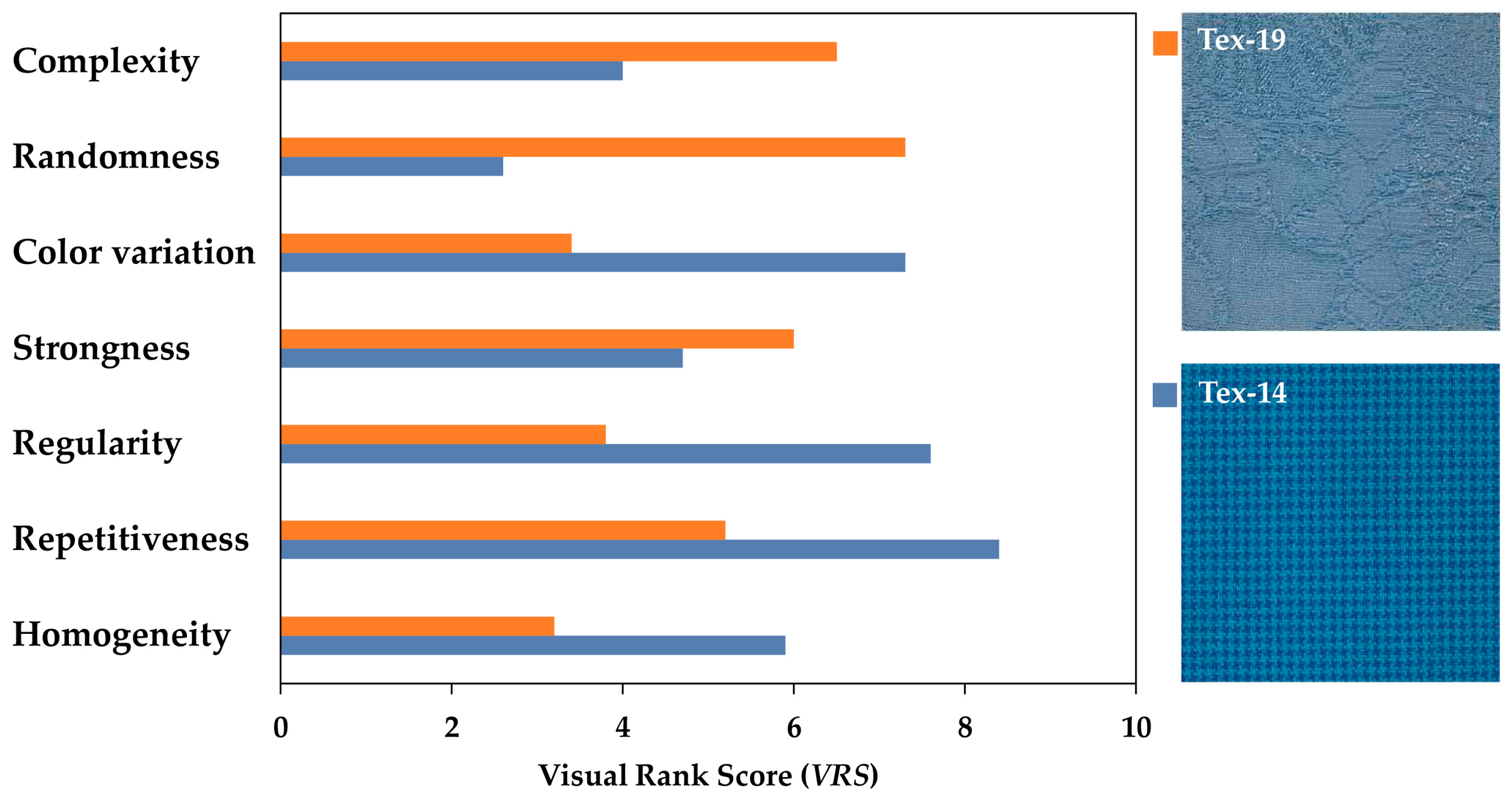
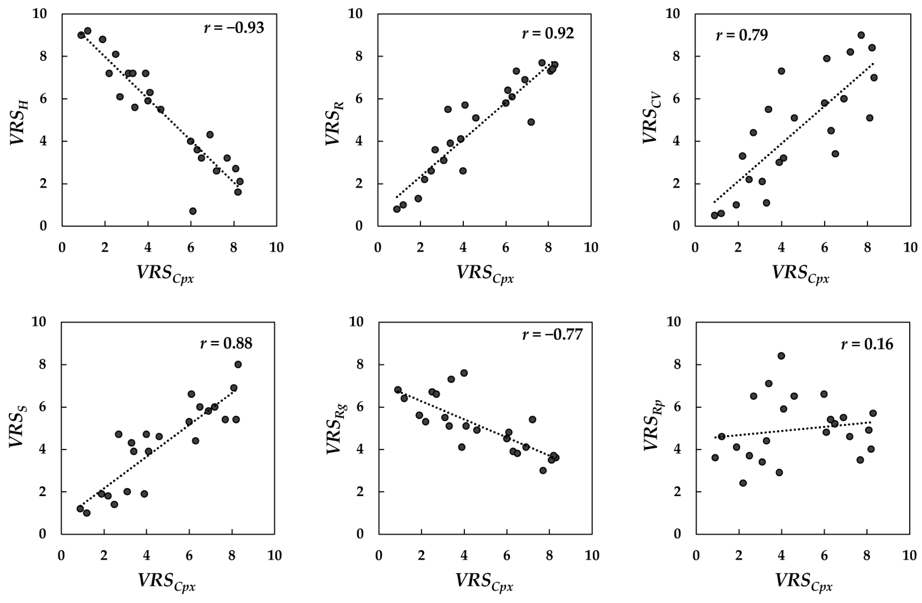
  • To investigate visual texture complexity and establish the degree to which it is correlated with homogeneity, randomness, repetitiveness, regularity, color variation, and strongness to better understand its perception. Visual texture complexity will be introduced and defined in detail in Section 4.1.
  • To investigate the possible relationships between visual texture complexity and some of the most popular and effective image texture measures.
  • To find the most suitable color space/s for the quantitative evaluation of visual texture complexity.
To this end, a number of first and second-order image statistics as well as the local binary pattern and Gabor features computed in different color spaces were used as potential measures for texture complexity, and possible existing correlations between such measures and visual ratings of texture complexity were sought. Section 2 of the paper introduces the detailed description of the texture measures used in this research. The remainder of the paper is structured as follows. Section 3 describes the research method implemented to perform the psychophysical experiments and the procedure to compute the texture measures of the textile images. In Section 4, the newly defined texture dimension of visual texture complexity is introduced and defined, and the relationships between the visual ratings of this attribute and the corresponding texture measures are presented. Section 5 discusses our results, and Section 6 presents our concluding remarks.

2. Quantitative Color Texture

Although there seems to be no comprehensive definition for texture in the literature, an image texture has been described as the spatial arrangement of colors or luminance elements in the image, which creates visual non-uniformity [37]. Fortunately, texture analysis techniques have made provisions for characterizing the texture of color images in terms of various texture measures [38]. Analyzing the texture of color images can be performed through different approaches: pure color analysis using color descriptors [39,40], grayscale texture analysis using texture features [41], and joint approaches that combine color and grayscale texture information [42,43]. Our preliminary experiments indicated that integrative co-occurrence matrix (CoM) features [43] and opponent Gabor features [44] as joint color-texture features, which combine information across different image channels, give rise to unsatisfactory results (i.e., weak correlations with the visual ratings of complexity). Therefore, we do not provide the details of these features in this section. In the following subsections, we provide our readers with a thorough description of the meaning and mathematical background behind some of the most popular image statistics and texture features we chose to use in this research. These include the first-order image statistics, co-occurrence matrix features as the second-order image statistics as well as the local binary pattern and Gabor features. We chose these texture features because they are simple and computationally cheap and have been shown to be efficient in texture classification tasks [44].

2.1. First-Order Statistical Texture Features—Image Descriptors

The statistical approach for texture analysis introduces the first-order statistics of color images [45]. Such image descriptors are the simplest features for characterizing textures and refer to statistical parameters such as the mean, standard deviation, and central moments. They are computed either directly from the image pixel values or from the image histogram. The former will be, hereafter, referred to as the global image descriptors while the latter will be referred to as the histogram-based image descriptors. Global image descriptors for a three-channel color image (e.g., an sRGB image) are the mean and standard deviation of the pixel values of each image channel.
The mean (µ) is the average of image pixel values and indicative of the general brightness of the image: the higher the µ, the brighter the image. The standard deviation (σ) is the measure of the spread in the pixel values around µ [46]. A higher σ indicates an image with higher contrast [45]. Here, the term “contrast” refers to the difference between the minimum and maximum pixel values, and not the more complex concept of perceptual image contrast [47]. Again, it must be noted that µ and σ are calculated as global image descriptors directly from the pixel values of each image channel.
As the histogram-based image descriptors, we chose skewness or the third central moment (m3), kurtosis or the fourth central moment (m4), energy (EnrgH), and entropy (EntpH). The skewness (m3) and kurtosis (m4) show how much the histogram is deviated from a normal distribution. The energy (EnrgH) indicates how pixel values are distributed in the image. A higher EnrgH means that the number of pixel values in the image is few, and the distribution is concentrated in only a small number of pixel values [45]. The entropy (EntpH) is a measure of how random the distribution of pixel values in the image is. This measure tends to vary inversely with EnrgH and has occasionally been considered as a measure of complexity in the texture analysis. One of the most commonly used definitions of entropy is Shannon’s entropy [33].
The first-order image descriptors are simple and straightforward, and invariant to the image spatial translation and rotation. However, they are slightly dependent on the viewing angle, sensitive to illumination change, and reliable merely under a constant illumination condition [40].

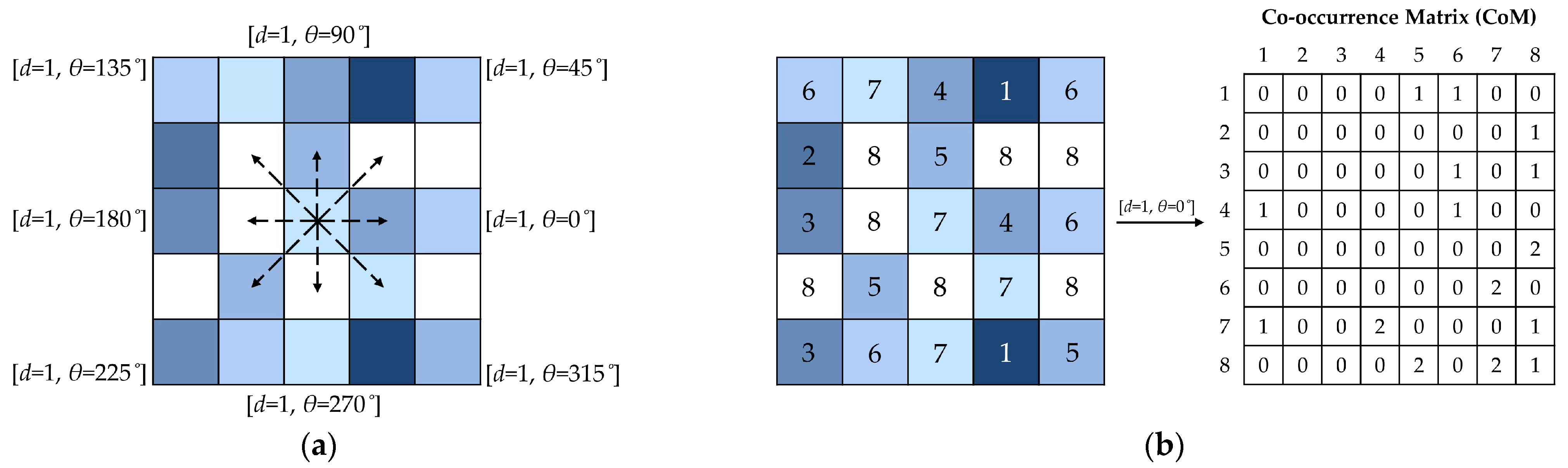
2.2. Second-Order Statistical Texture Features—Co-Occurrence Matrix (CoM) Features

The first-order statistics provide information about the distribution of the image pixel values. However, they are unable to provide any information about the relative positions of such pixels in the image. Examining the spatial relationship between pairs of pixels across the image can be conducted through the second-order statistical features. Co-occurrence matrix (CoM) is one of the most well-known second-order statistical operators for texture analysis [32]. A CoM is a two-dimensional matrix comprising the probabilities of occurring pairs of pixels with specific pixel values at a particular displacement of distance d and rotation angle θ. Figure 1a illustrates the displacement rules to generate CoMs with the distance d = 1 pixe, and equally-spaced rotation angles θ ∈ {0, 45, 90, 135, 180, 225, 270, 315}°. An example of a CoM for [d = 1, θ = 0°], after reducing the image bit depth to n = 8 through quantization, is depicted in Figure 1b.
A number of statistics can be derived from the CoM. Haralick et al. [32] proposed fourteen simple and rather intuitive CoM features for texture classification. However, it has been demonstrated that some of these features are highly correlated and only five of them (i.e., energy, contrast, correlation, entropy, and homogeneity could be sufficient for texture analysis purposes) [42].
The CoM energy (EnrgCoM), also known as the angular second moment, indicates how uniformly pixel values are distributed in the image. The CoM contrast (ContCoM) is a measure of local intensity variations in image pixel values. The CoM correlation (CorrCoM) is a measure of linear dependency between the pixel values at specific positions in the image. The CoM entropy (EntpCoM) measures the extent to which pixel values are randomly distributed in the image. The CoM homogeneity (HomgCoM), also known as the inverse difference moment, measures the homogeneity of the image [48].
CoMs are rather easy to implement and have proven to be very efficient in various texture analysis tasks [49,50,51,52]. Although CoM features could be made invariant to rotation and scaling, they are highly dependent on illumination: changing illumination condition results in different image pixel values, and it affects the resulting CoM [53]. To address this limitation, the local binary pattern (LBP) operator was developed as a “grayscale-invariant” texture analysis tool [54].

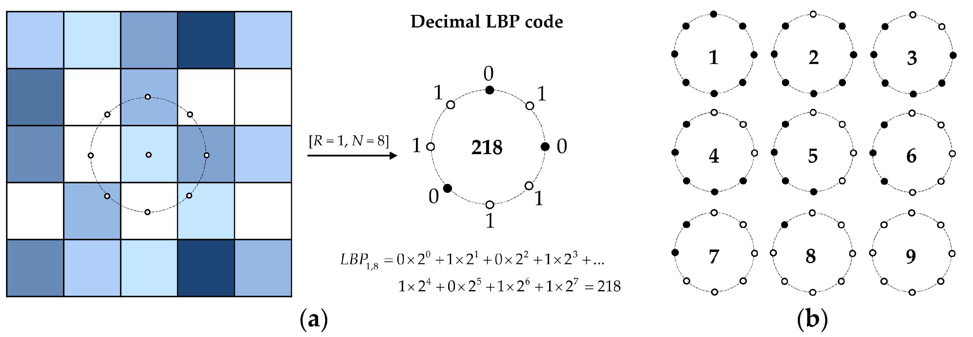
2.3. Local Binary Pattern (LBP) Features

Local binary pattern (LBP) is a powerful grayscale and rotation-invariant texture operator that has found widespread applications in texture analysis and pattern recognition due to its simplicity and discriminative efficiency [55,56]. For each image pixel, the LBP is derived from the signs of the differences between the value of that pixel, and the values of the N neighboring pixels surrounding it at the radius R. Figure 2a illustrates an example of generating the decimal LBP code for a pixel using its N = 8 neighboring pixels at the radius R = 1 pixel. Using the signs of the differences in the pixel values instead of their absolute values makes the LBP invariant to any monotonic changes in the image pixel values.
For a neighborhood of N pixels, the LBP operator produces 2N different binary patterns. Ojala et al. [54] observed that amongst all of the possible 2N binary patterns, only N + 1 patterns are associated with the most fundamental micro-structures of the texture such as bright points, dark points, edges, and corners. These patterns are known as uniform LBPs. Figure 2b shows the nine possible uniform binary patterns when N = 8, as proposed in [54]. The remaining patterns are categorized as non-uniform ones. The frequencies of the occurrence of uniform and non-uniform patterns in the image texture are recorded as a feature vector and represented as the LBP histogram.

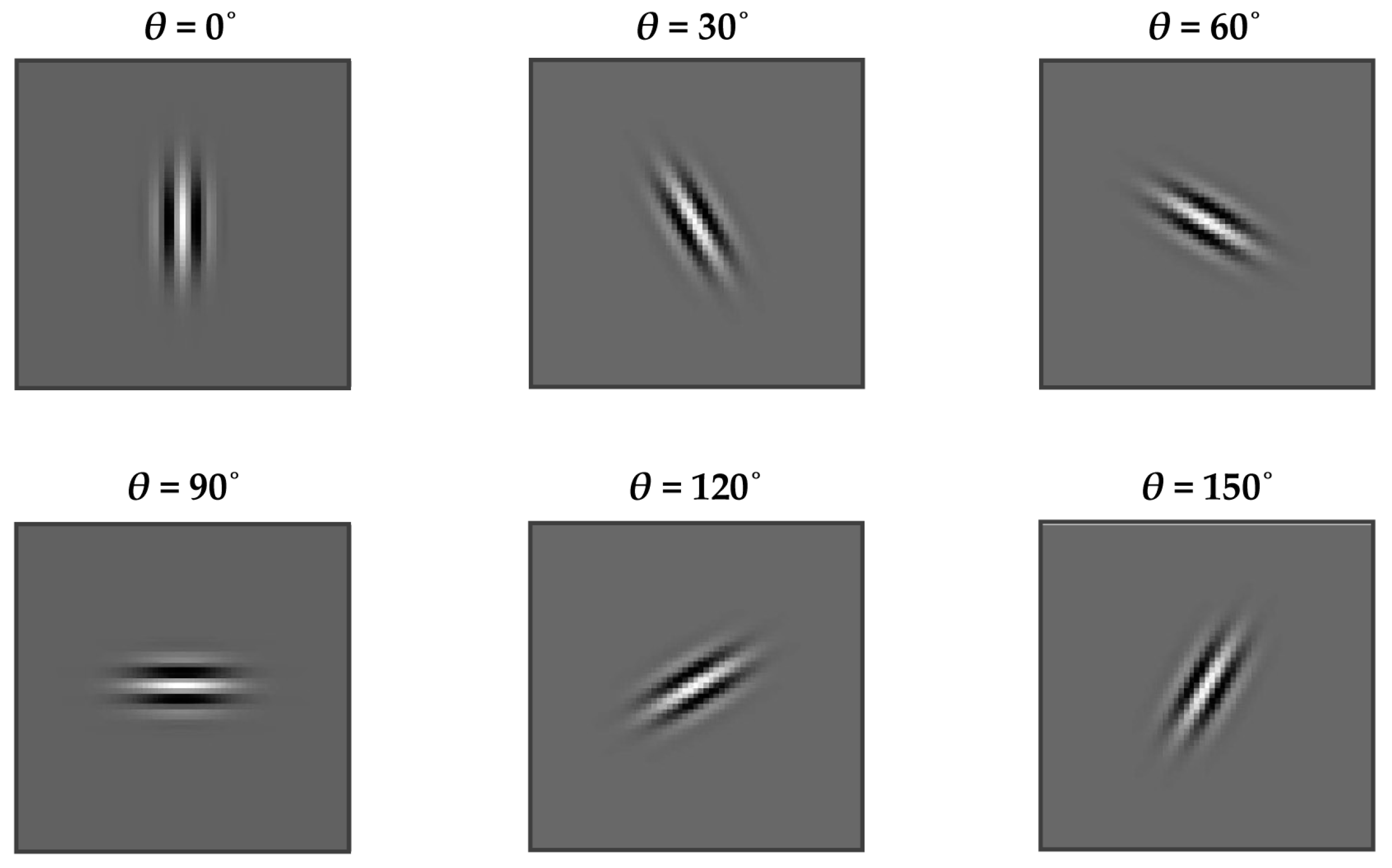
2.4. Gabor Filtering

Frequency is an essential property of many textures. Gabor filtering provides means for analyzing the image texture by decomposing it into components of varying spatial frequency (F) and orientation (θ). A Gabor filter in the spatial domain is obtained by modulating a two-dimensional complex sinusoid carrier with a two-dimensional Gaussian envelope [57]. Figure 3 shows the visualizations of the real part of the Gabor function with the frequency F = 0.18 and orientation angles θ ∈ {0, 30, 60, 90, 120, 150}°, which were used to extract the Gabor features of the image textures in this research.
The crucial step in implementing Gabor filtering for texture analysis is designing the Gabor filter bank. A filter bank comprises a number of Gabor filters with different spatial frequencies and orientations, obtained by presetting the filter parameters. After convolving the image texture by the filter bank, the mean and standard deviation of the energy of the filtered image is used as the Gabor texture features [57]. The Gabor filtering technique has been found to be very efficient in various texture analysis tasks. However, it suffers from being sensitive to changes in illumination as well as being computationally intensive [58].

3. Materials and Methods

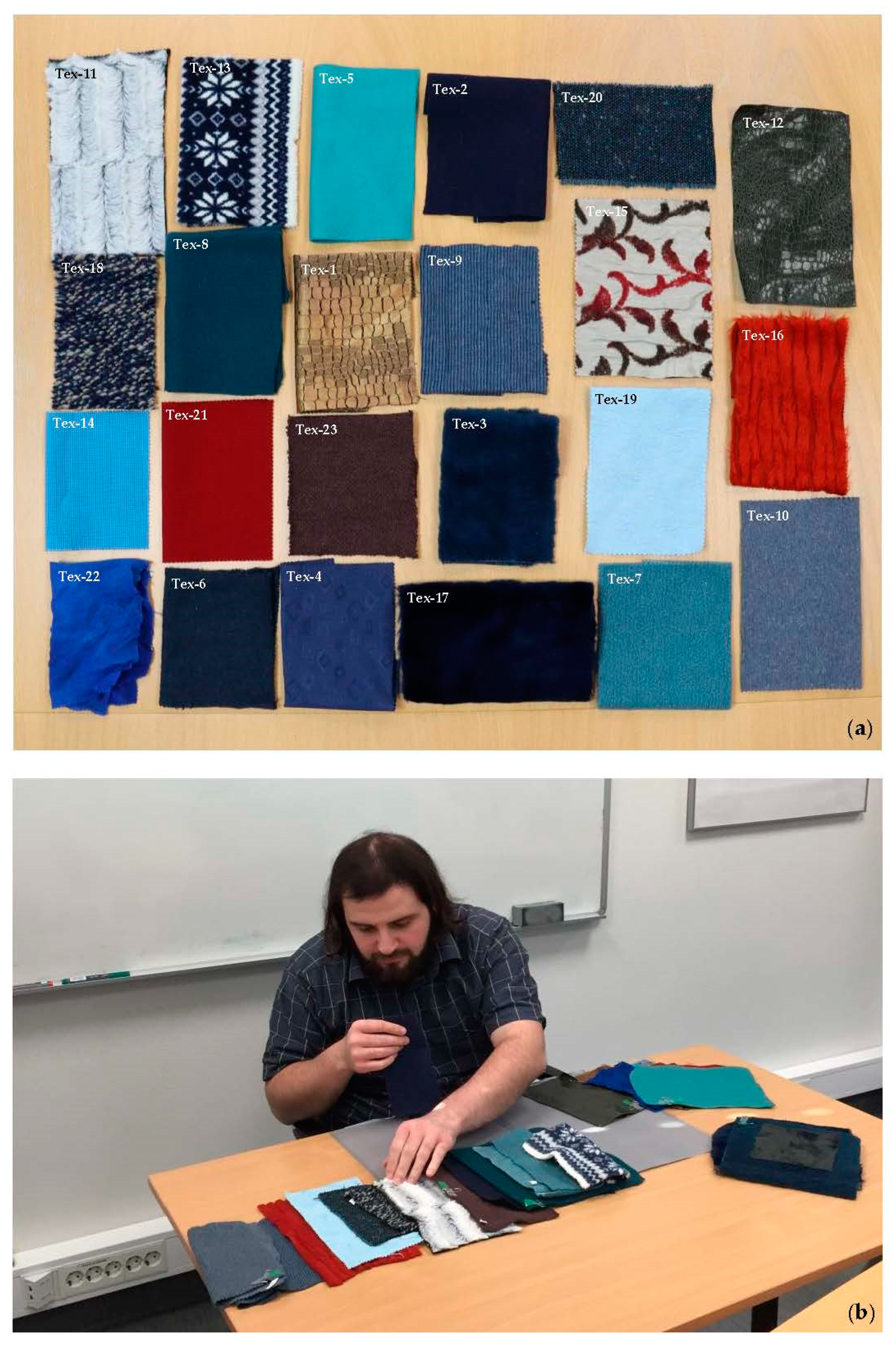
3.1. Visual Assessment of Texture of the Textiles

As discussed in our previous work [36], the results of a verbal description experiment using 52 textile fabrics revealed that observers tend to use some essential tactile and visual cues to evaluate the textural appearance of the textiles. These cues were smoothness, softness, homogeneity, geometric variation, randomness, repetitiveness, regularity, color variation, strongness, and complexity. Based on the observers’ statements, we found that smoothness, softness, and geometric variation were mainly evaluated by touch, while the rest of the attributes were evaluated merely visually.
To build a foundation upon the results of [36] for more in-depth research on texture perception, we used the same textile samples in the present study. Having determined the most tangible visual attributes of texture appearance of the textiles, the next step was to quantify these attributes. The rank ordering method [59] was employed for this purpose. It was found during the verbal description experiment that the main color of the textile sample had no significant impact on its texture evaluation by the observers. For instance, the observers would describe the texture of a fur in blue the same way as they would describe the texture of that fur in red. Therefore, a subset of 23 fabrics with more or less the same main color, but different textures was selected from the sample set for the rank ordering experiments. A photograph of the selected fabrics is depicted in Figure 4.
Ten observers including seven males and three females, aging between 24 to 36 years old, with normal to corrected to normal color vision (pre-tested by the Ishihara’s test for color deficiency) participated in the rank ordering experiments.
The observers were given ample opportunity to understand the purpose of the research and their right to withdraw from the experiment before they gave their informed consent to participate. None of the observers were experts in the field of texture appearance. The rank ordering experiments were conducted in a meeting room with large windows providing natural daylight illumination. The room was also equipped with daylight fluorescent tubes. The observers sat at a table that was partially covered with a medium gray paperboard to provide a neutral background on the working area. The viewing geometry (i.e., the angle between the observer’s viewing direction and the surface normal of the table) was approximately 45°. The viewing distance (i.e., the distance between the observer’s eyes and the surface of the table-where the samples were placed) was 40 cm. The combined natural and artificial illumination on the working area had the correlated color temperature (CCT) and illuminance of approximately 6000 K and 500 lx, respectively.
After introducing written instructions about the experiment, the observers were presented with the 23 textiles. Although none of the observers was a native English speaker, they could understand and speak the English language very well. Therefore, the instruction was given in English. However, if they were unfamiliar with the meaning of an attribute, they were allowed to use online dictionaries to find the meaning. The written instructions on the experiment is given in Appendix A.
The observers had the task of ranking the textiles on the table, according to how strongly they represented the seven visual texture attributes (i.e., complexity, homogeneity, randomness, repetitiveness, regularity, color variation, and strongness) from the lowest to the highest of each attribute. The observers were intentionally not provided with an explicit definition of the texture or texture attributes. In fact, they were expected to use their own knowledge and understanding of texture. They were allowed to freely touch the sample, however, they had to maintain the viewing distance throughout the experiment. Since the experiment was not a forced-choice task, the observers could assign the same rank order to several samples, if needed. Figure 4 also shows an observer performing the rank ordering experiment. Each observer completed the task without a time restriction, although they would tend to finish the task in approximately one hour.

3.2. Image Acquisition Procedure

As mentioned previously, one of the primary objectives of this study was to investigate the possible relationships between the texture complexity and the most popular and effective image texture measures. To compute such texture measures, we acquired the sRGB images of the selected 23 textiles. The textile fabrics used in this study were part of the “Textile” class used by the HyTexila texture database [60]. The hyperspectral images of the textiles were acquired using a HySpex VNIR-1800 hyperspectral camera (Norsk Elektro Optikk AS, Oslo, Norway). The acquisition setup and procedure are fully described in [60]. Each textile was acquired by the camera to obtain a radiance image for 186 spectral bands.
The radiance images were converted to the reflectance images using the estimated spectral power distribution of the camera’s illumination system. Finally, the reflectance images were converted to sRGB images for the CIE standard illuminant D65 and CIE 1931 color matching function and cropped into images of 1024 × 1024 pixels.
For our computations of image texture to be reproducible by other researchers, we performed the color calculations using D65, which was the closest CIE standard illuminant to our illumination condition in the experiment room. To ensure that the color-difference caused by the difference in illumination condition was perceptually insignificant, we measured the average CIELAB 1976 color-difference of the two conditions on the 24 color patches of the X-Rite color checker [61]. The average CIELAB 1976 color-difference was 0.86, which is below the just noticeable difference (JND) threshold [62]. This indicates a negligible perceptual difference between the two illumination conditions. Figure 5 shows the sRGB images of the textiles used to compute the texture measures. It must be noted that the textiles in Figure 5 were sorted in ascending order in terms of texture complexity according to their visual rank score (VRS) given by the observers. Section 4.1 provides detailed information on how the VRS was computed.

3.3. Computing the Image Descriptors and Texture Features of the Textile Images

Although the output of the majority of image capturing devices is color images in terms of red, green, and blue signals in the so-called RGB space, with the variety of standardized color spaces available, the question of which color space is more effective for a particular texture analysis task always remains [63]. To find the best representative color space/s for computing the image descriptors and texture features of the textile images, we chose the five popular color spaces in computer vision [64] (i.e., sRGB, HSV, YCbCr, Ohta’s I1I2I3, and CIELAB). They have also been used in several texture analysis and classification studies and have shown a good performance amongst the many color spaces available [65,66,67]. We followed a similar principle to find the most suitable color space/s for our application.
One of the advantages of the HSV, YCbCr, I1I2I3, and CIELAB color spaces compared to sRGB is that they allow for separate treatment of the luminance and chrominance components of the image [68]. The formulas used to transform the sRGB images of the textiles to HSV, YCbCr, I1I2I3, and CIELAB color spaces are given in Appendix B.
The six first-order image descriptors (i.e., global µ and σ), together with histogram-based m3, m4, EnrgH and EntpH, were computed for each channel of the textile images in the sRGB space. Additionally, global µ and σ were computed for each channel of the images in the HSV, YCbCr, I1I2I3, and CIELAB color spaces. To compute the CoM features, the CoMs were generated for nine distances d ∈ {1, 5, 10, 15, 25, 50, 100, 150, 250} pixel/s and eight orientation angles θ ∈ {0, 45, 90, 135, 180, 225, 270, 315}° for each channel of the textile images in the five color spaces. The energy, contrast, correlation, entropy, and homogeneity of each CoM were then calculated. To obtain the rotation-invariant CoM features, the calculated features were averaged over the eight orientation angles.
Similarly, the LBP histograms were generated for eight neighboring pixels, N = 8, and nine radii R ∈ {1, 5, 10, 15, 25, 50, 100, 150, 250} pixel/s for each channel of the textile images in the five color spaces. A preliminary correlation analysis indicated that increasing N along with R had no significant impact on the results. Therefore, all LBP computations were performed with N = 8. For N = 8, the LBP histogram had ten bins, where the first nine bins were associated with the nine uniform LBPs (see Figure 2b) and the tenth bin was associated with the combination of all possible non-uniform LBPs. The histogram frequencies were used as the LBP features.
For the Gabor features, a bank of 36 Gabor filters were designed using six frequencies (nF = 6) (i.e., F ∈ {1, 0.7, 0.5, 0.35, 0.25, 0.18} with the maximum frequency Fm = 1) and six orientation angles (nO = 6) i.e., θ ∈ {0, 30, 60, 90, 120, 150}° (see Figure 3). As recommended in [34], the frequency ratio Fr was half-octave frequency spacing (Fr = 2 ) and the smoothing parameters were γ = η = 0.5. The mean and standard deviation of the energy of the filtered images were averaged over the six orientation angles to obtain the rotation-invariant Gabor features of the textile images.

4. Results

The outcome of the visual assessment experiments was first used to compute the visual rank scores (VRS) of the seven texture attributes of the textiles, and subsequently their relationships. Section 4.1 describes how VRS was computed and used to define visual texture complexity. Section 4.2 presents the results of investigating the relationships between the VRS of the complexity of the textiles, and the corresponding image descriptors and texture features (as introduced in Section 2) computed for the textile images in the sRGB, HSV, YCbCr, I1I2I3, and CIELAB color spaces.

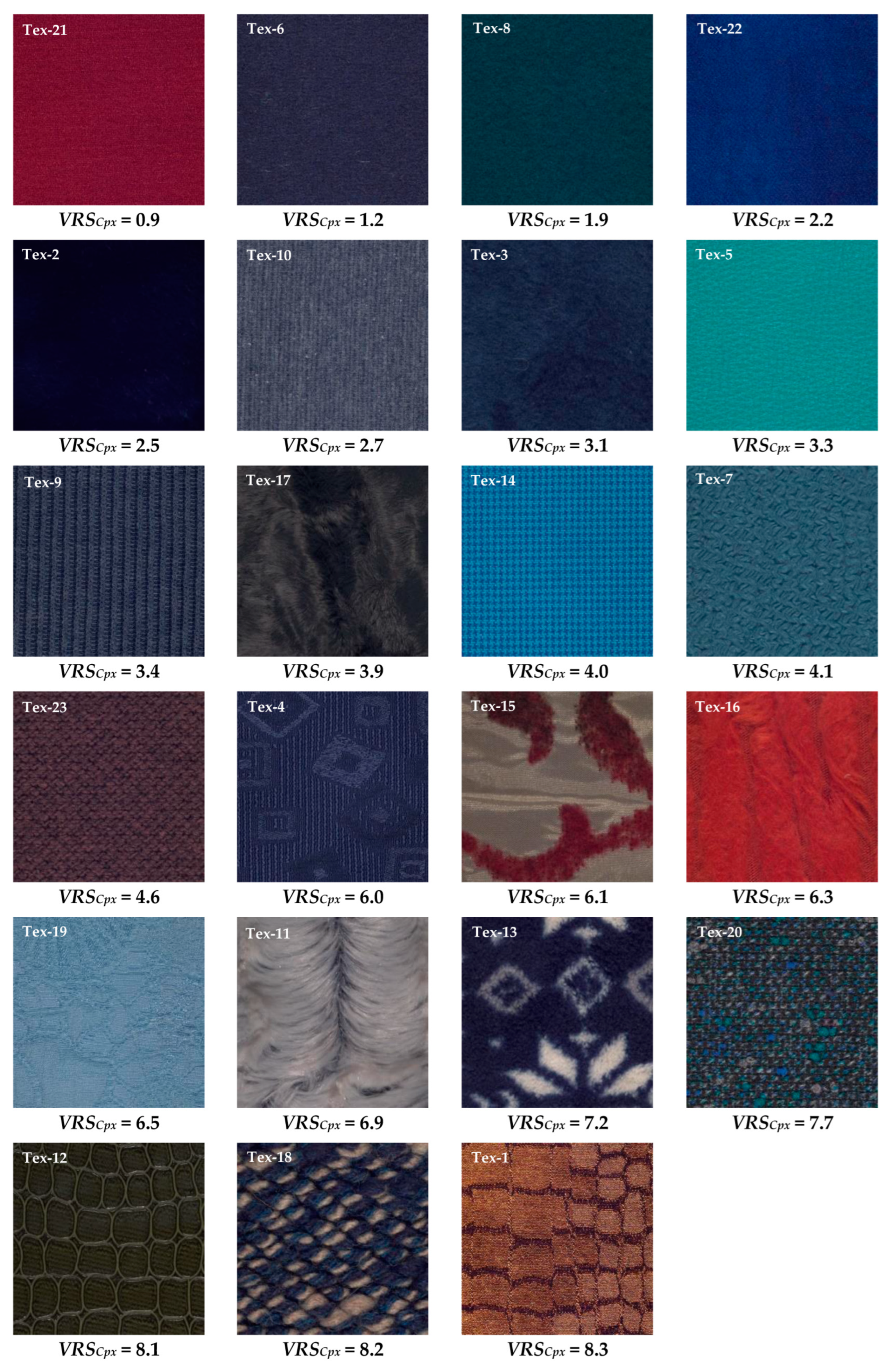
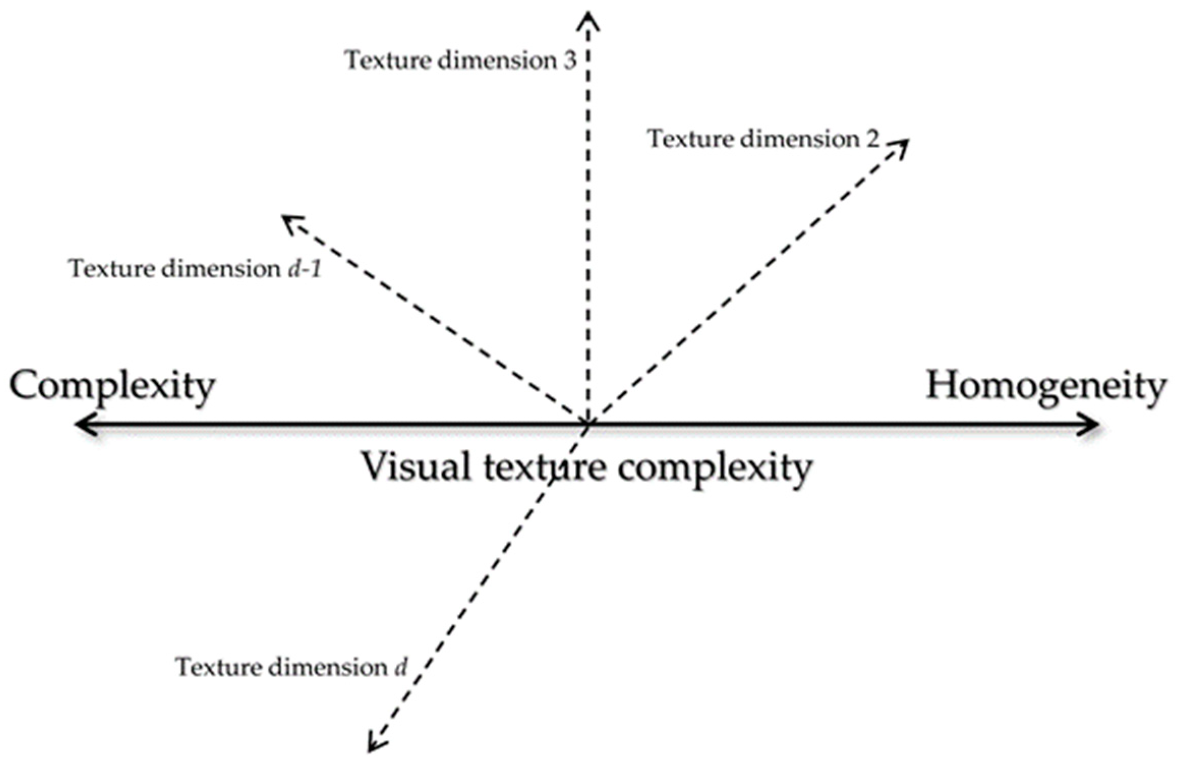
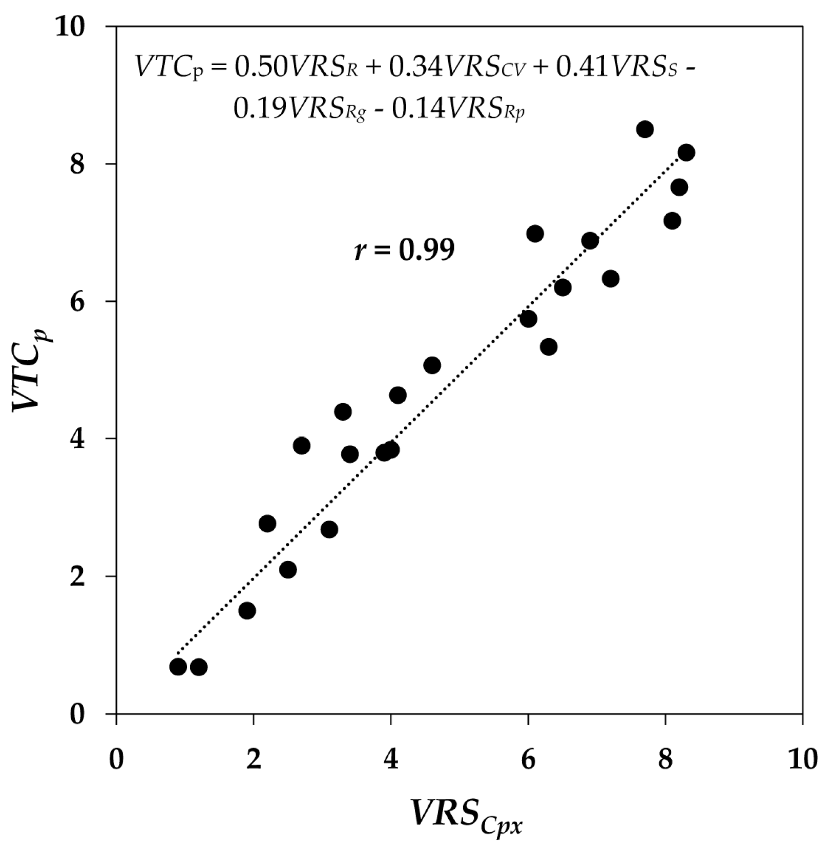
4.1. Visual Texture Complexity

The order of ranking of each textile was recorded for each observer, and first used to determine the accuracy of the observers in their assessments. To evaluate the extent of the observers’ accuracy in terms of the intra-observer and inter-observer variability, the standardized residual sum of squares (STRESS) metric [69] was used. The percent STRESS values were always between 0 and 100, where values of STRESS near zero indicate less variability. For intra-observer variability, the average STRESS value of the ten observers was 24 STRESS units. This value indicates that all observers were reasonably internally consistent. The average inter-observer variability of the ten observers was 38 STRESS units, which was larger than the average intra-observer variability (i.e., 24 STRESS units), as might be expected. This value indicates a reasonable degree of consistency between the observers. The visual rank score (VRS) of each textile was then calculated separately for each texture attribute using Equation (1) [59], and linearly re-scaled to be within the range of 0–10 for better visualization:
V R S = 1 S ( T 1 ) t = 1 T t Q t
where S is the number of observers; T is the number of textile samples; and Qt is the number of times the textile t is ranked at position t. Figure 6 compares two of the textiles (i.e., Tex-19 and Tex-14 )in terms of their VRS computed for the seven texture attributes.
The VRS of complexity, randomness, color variation, strongness, regularity, repetitiveness and homogeneity will be, hereafter, denoted as VRSCpx, VRSR, VRSCV, VRSS, VRSRg, VRSRp, and VRSH for brevity. The sRGB images of the textiles, sorted according to their VRSCpx, from the lowest to the highest VRSCpx, are depicted in Figure 5. A comparison of the VRSCpx values in Figure 5 indicates that the textiles with a homogeneous structure were judged as less complex, while those with a more random structure and stronger embedded details were considered as more complex by the observers.
In order to find out how the texture complexity is related to the other visual texture attributes, the correlations between VRSCpx and VRSR, VRSCV, VRSS, VRSRg, VRSRp, and VRSH were determined in terms of the correlation coefficient (r) for the 95% confidence interval (p < 0.5). Scatter plots of such correlations are depicted in Figure 7.
Analyzing the correlations in Figure 7 showed that there were positive linear correlations between VRSCpx and the corresponding VRSR (r = 0.92), VRSS (r = 0.88), and VRSCV (r = 0.79). Additionally, there were negative correlations between VRSCpx and the corresponding VRSH (r = −0.93) and VRSRg (r = −0.77). The correlation coefficient (r) for repetitiveness was positive but significantly low (due to the fact that there are not many samples with a repetitive texture in the sample set used). Such correlations indicate that when the texture is random or strong, or has a high content of color non-uniformity, it could be perceived as complex. On the other hand, when the texture is homogenous or regular, it could be perceived as less complex. To find the possible underlying relations between these attributes, principal component analysis (PCA) [70] was conducted on the VRS values. It was found that the first two principal components with eigenvalues of 31.3 and 8.4, respectively, correspond to 90% of the data variance. These coefficients are depicted in Table 1.
Comparing the PCs in Table 1 showed that PC1 had the strongest negative and positive associations with complexity (PC1 = −0.42) and homogeneity (PC1 = 0.44), respectively. The PC1, however, was much smaller for repetitiveness (PC1 = −0.08) and regularity (PC1 = 0.16), indicating that the two attributes did not correlate with PC1. On the other hand, PC2 had the strongest positive associations with repetitiveness (PC2 = 0.47) and regularity (PC2 = 0.46).
Assuming that texture (e.g., color and gloss) is a multidimensional appearance attribute, the PCA results might suggest that complexity and homogeneity could be essentially the underlying attributes of the same visual texture dimension (described by PC1), with complexity at the negative extreme and homogeneity at the positive extreme of this dimension. We chose to call this dimension visual texture complexity. In other words, we can assume a d-dimensional hypothetical perceptual texture space with visual texture complexity as one of its dimensions. This dimension holds both complexity and homogeneity of texture. Figure 8 illustrates such a texture space. The PC1 values demonstrate that color variation, randomness, and strongness (with respective PC1 values −0.40, −0.37, −0.34) are strongly related to this dimension.
Considering the strong linear correlation between VRSH and VRSCpx (see Figure 7), and the large-absolute-PC1 obtained for both VRSH and VRSCpx, we could use either of the scores as the visual ratings of visual texture complexity. However, preliminary correlation analysis showed that unlike VRSCpx, VRSH was inversely correlated with the computed texture measures. Therefore, we chose VRSCpx as the visual ratings of visual texture complexity for further correlation analysis in this paper.
To quantify the extent to which each attribute contributes to visual texture complexity, the multivariate regression method was used to model the correlation between VRSCpx and the VRS of the rest of the attributes using the generic formula in Equation (2):
V T C p = k 1 [ V R S R ] + k 2 [ V R S C V ] + k 3 [ V R S S ] + k 4 [ V R S R g ] + k 5 [ V R S R p ]
where VTCP is an intermediate variable defined to hold the ‘predicted’ visual texture complexity values, computed as the weighted sum of VRSR, VRSCV, VRSS, VRSRg, and VRSRp, and ki; i = 1, 2, …, 5 are coefficients to express the contribution of each attribute to VTCP. Like visual texture complexity, VTCP is desired to be highly related to VRSCpx. Therefore, the coefficients ki in Equation (2) were determined in such a way that the mean squared error (MSE) of the correlation between VRSCpx and the corresponding computed VTCp values for the 23 textiles were minimized. The best linear correlation was achieved when k1, k2, k3, k4, and k5 were 0.50, 0.34, 0.41, −0.19, and −0.14, respectively. Figure 9 presents such a linear correlation between VRSCpx and VTCp. These coefficients demonstrate that randomness of texture with k1 = 0.50, followed by strongness with k3 = 0.41 and color variation with k2 = 0.34 had the highest positive contributions to VRSCpx and hence visual texture complexity: the higher these attributes are, the higher the visual texture complexity will be. On the other hand, greater regularity and repetitiveness contribute to lower visual texture complexity.
Given that texture is perceived as the frequency and spatial arrangement of color and/or luminance elements over the surface of a material [37], the randomness, strongness, regularity, and repetitiveness of texture could mainly be associated with the frequency and spatial distribution of such elements, regardless of their color, while color variation could be mainly associated with the frequency and diversity of color elements. These elements, also known as ‘texture primitives’ and ‘textons’ in the literature, are the smallest geometrical parts constituting a two-dimensional texture. Based on these correlations, visual texture complexity can be defined as the perceived degree of disorder or randomness in the distribution of color and luminance elements over the surface of a material, which depends on the size, shape, amount, and arrangement of such elements. We observed, during the visual assessment experiments, that a complex texture might be effortlessly discernable by the observer due to being salient and strong, but it might not necessarily be understandable, interpretable, or definable due to its random structure.

4.2. Correlation between Visual Texture Complexity and Image Descriptors

All image descriptors were linearly re-scaled to be within the same range as the VRS data (i.e., 0–10) for better visual comparison.

4.2.1. sRGB Space

The R, G, and B channels in the sRGB space are highly correlated. This characteristic of the sRGB space makes it unsuitable for the individual evaluation of the effectiveness of each channel. Additionally, unlike the other color spaces investigated in this work, the luminance and chrominance information of sRGB images cannot be treated separately [71]. To obtain an approximation of luminance information in sRGB space, the sRGB images of the textiles were converted into the corresponding intensity images (see Appendix B).
Global µ and σ as well as histogram-based m3, m4, EnrgH, and EntpH were calculated separately for the R, G and B channels as well as the corresponding intensity images of the textiles, and re-scaled to be within the range 0–10. Correlations between VRSCpx of the textiles and their respective computed image descriptors were then analyzed in terms of the correlation coefficient (r) for the 95% confidence interval (p < 0.5) separately for the R, G, and B channels and the intensity images. The bar graph in Figure 10 compares these correlation coefficients (r). The correlation coefficients (r) in Figure 10 showed that amongst all of the image descriptors, global σ, as a measure of image contrast, followed by EntpH as an indicator of how random the distribution of image pixel values is, exhibited the highest positive correlations with VRSCpx. EnrgH, as a measure of how few the number of pixel values in the image is, had a negative correlation with the visual data. On the other hand, there was no correlation between the global µ and the visual data. This proves that the mean is not a good candidate for quantifying the visual texture complexity, as expected. Central moments, m3 and m4, also exhibited weak correlations with the visual data.
The results in Figure 10 also revealed that each image channel tended to have a different performance in quantifying the visual texture complexity in a way that the highest correlations always belonged to the G channel, while the R channel always had the lowest correlations. This behavior might be attributed to the greater amount of useful information and less noise and blurriness provided by the G channel. Moreover, this could be due to the fact that the 23 image textures had a dominant blue-green color.
As mentioned previously, due to high cross-correlations between the R, G, and B channels in sRGB, comparing the image chromatic and achromatic/luminance components in terms of their contribution to visual texture complexity is not straightforward in the sRGB space. However, as can be seen in Figure 10, the image descriptors calculated for the intensity images of the textiles exhibited correlations that were fairly comparable with those of the best performing channel (i.e., the G channel). Scatter plots of the global σ and EntpH of the sRGB intensity images against the corresponding VRSCpx of the textiles are also depicted in Figure 10. Overall, the results indicate that the luminance content of the images might provide sufficient information for the objective quantification of texture complexity. Moreover, the choice of the image channel is a crucial step when working with color images in the sRGB space.

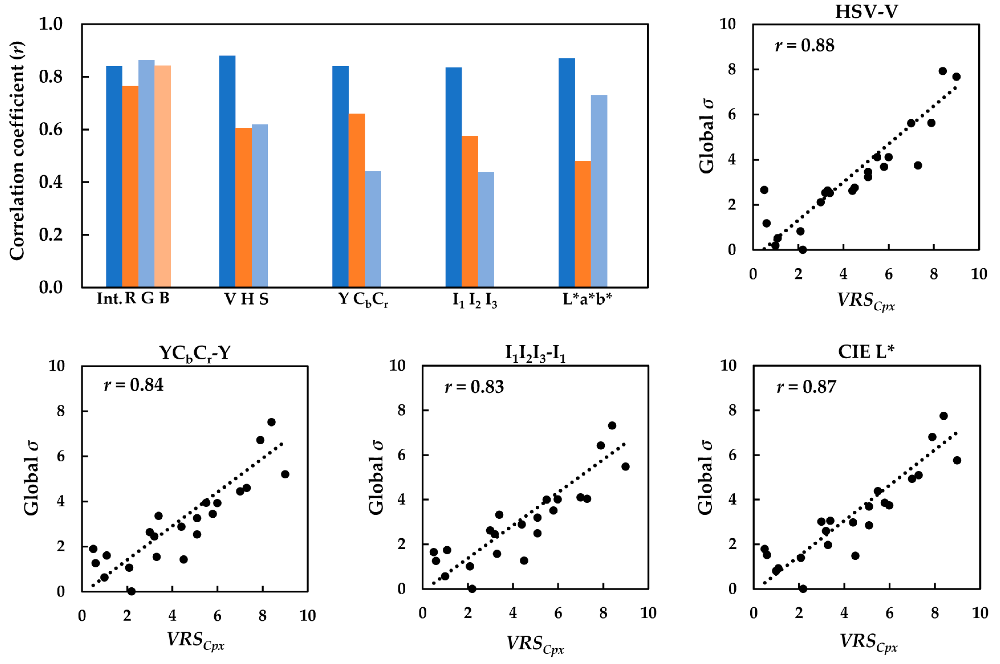
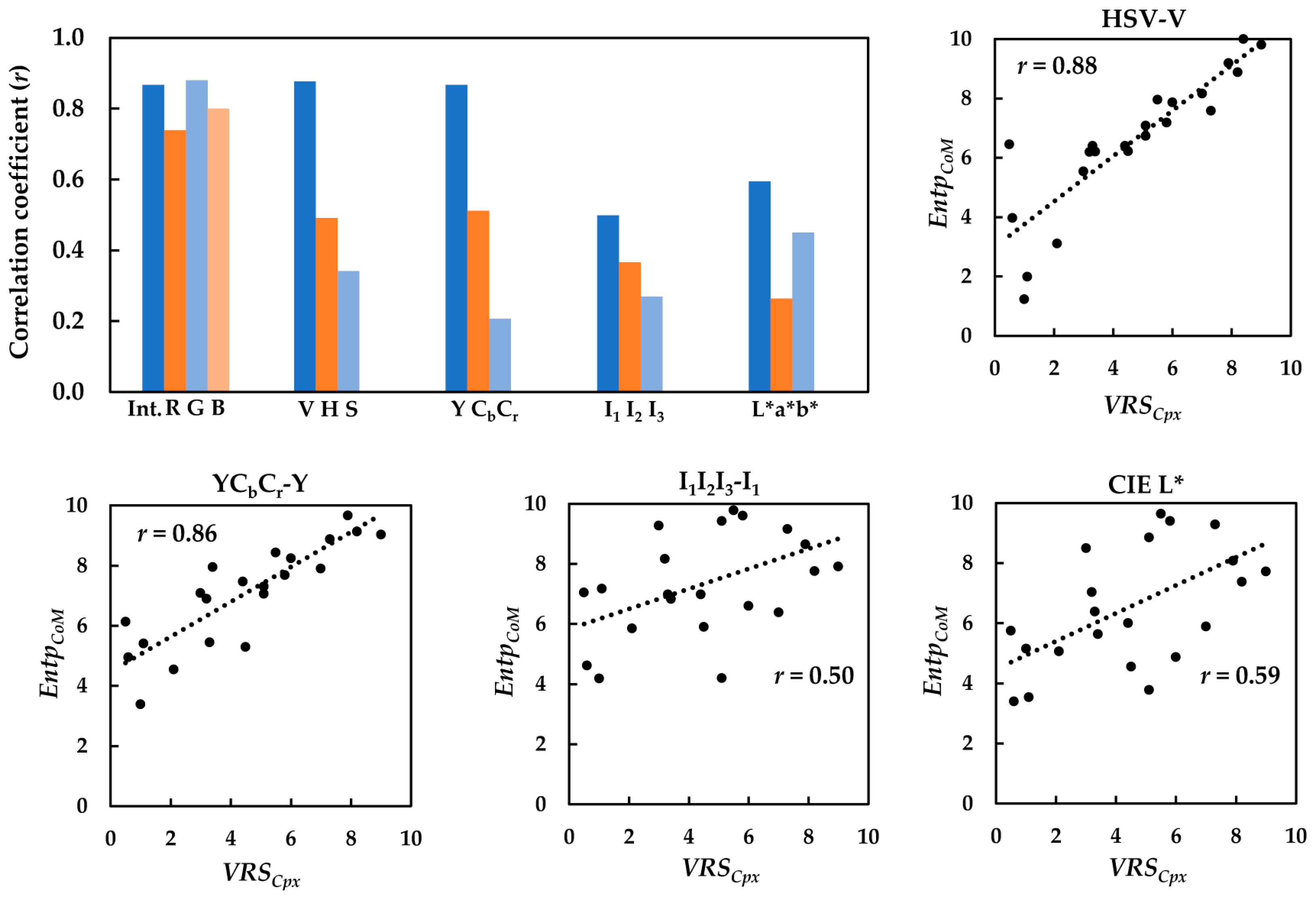
4.2.2. Luminance–Chrominance Color Spaces

Transformations of the sRGB images in HSV, YCbCr, I1I2I3, and CIELAB (for CIE standard illuminant D65) color spaces were employed to compute the global image descriptors. The formulas for performing such transformations are given in Appendix B. Unlike the sRGB space, luminance–chrominance color spaces allow for the separate treatment of the color and luminance components of color images. V, Y, I1, and CIE L* are luminance channels, while H and S, Cb, and Cr, I2 and I3, and CIE a* and b* are the chrominance channels in the HSV, YCbCr, I1I2I3, and CIELAB color spaces, respectively. We must remind our readers that the term ‘chrominance’ here is different to that of ‘chroma’, as one of the three dimensions of color in the Munsell color system. Interested readers are referred to [64] for more information about the standardized color spaces available for image analysis.
Correlations between the global µ and σ of the luminance and chrominance channels of the images with the respective VRSCpx were determined in terms of the correlation coefficient (r). Similar results were observed: the global σ performed significantly better than the global µ in terms of its relationship with the visual data. The bar graph in Figure 11 compares the correlation coefficients (r) of the relationships between the global σ of the images and VRSCpx of the textiles, separately, for the luminance and chrominance channels in all five color spaces.
Analysis of the correlations in Figure 11 clearly showed that the global σ of the luminance channel gave rise to markedly higher correlation coefficients (r) compared to the chrominance channels. In other words, there seems to be a strong linear relationship between the standard deviation of the image luminance channel and its texture complexity, regardless of the color space used. Scatter plots of the best performing image descriptor (i.e., global σ computed for luminance channel of the images in HSV, YCbCr, I1I2I3 and CIELAB) against the corresponding VRSCpx are also presented in Figure 11.
Although the correlation coefficients (r) obtained for the two chrominance channels of the images were lower, one always tends to result in a better relationship between the visual data and the computed texture feature. For instance, CIE b* resulted in a higher correlation coefficient (r) compared to CIE a*. Again, this could be attributed to the dominant blue-green color of the images.

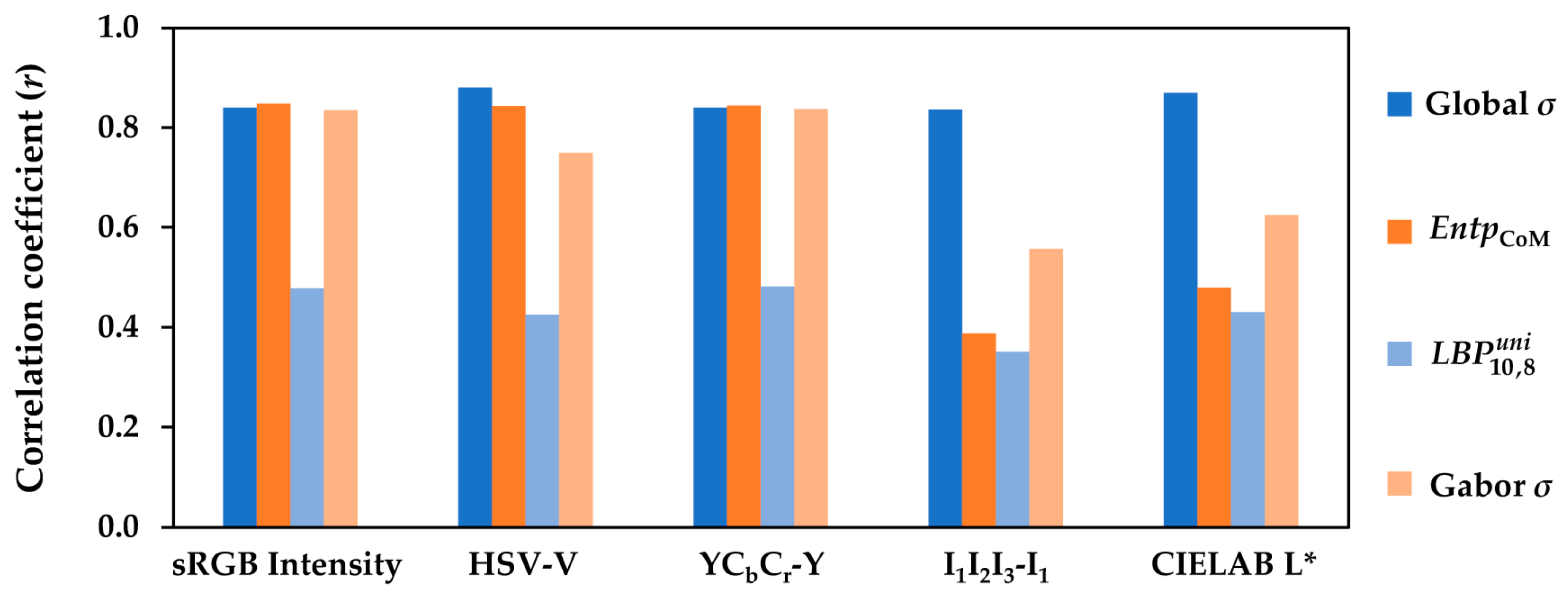
4.3. Correlation between Visual Texture Complexity and Texture Features

All texture features were linearly re-scaled to be within the range of 0–10 for a better visual comparison with the visual data.

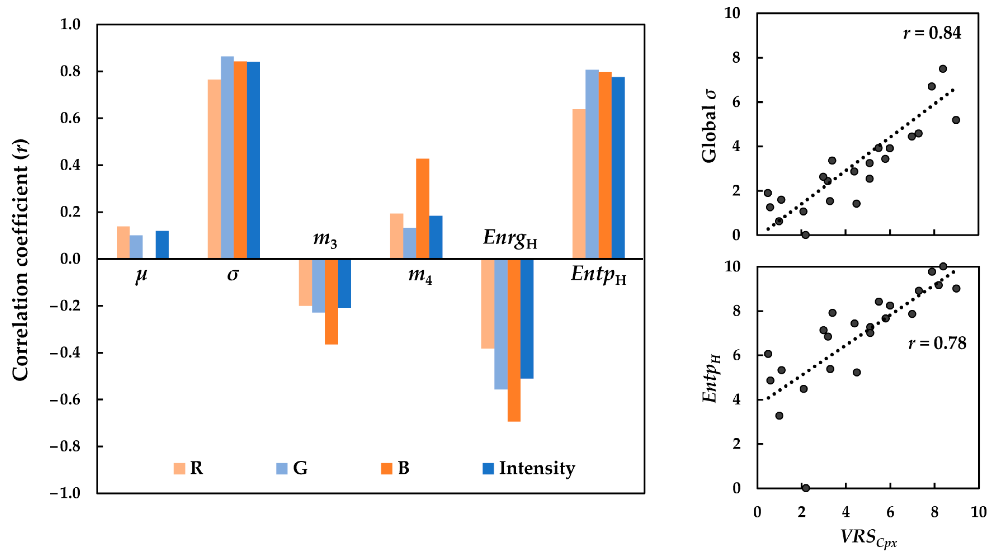
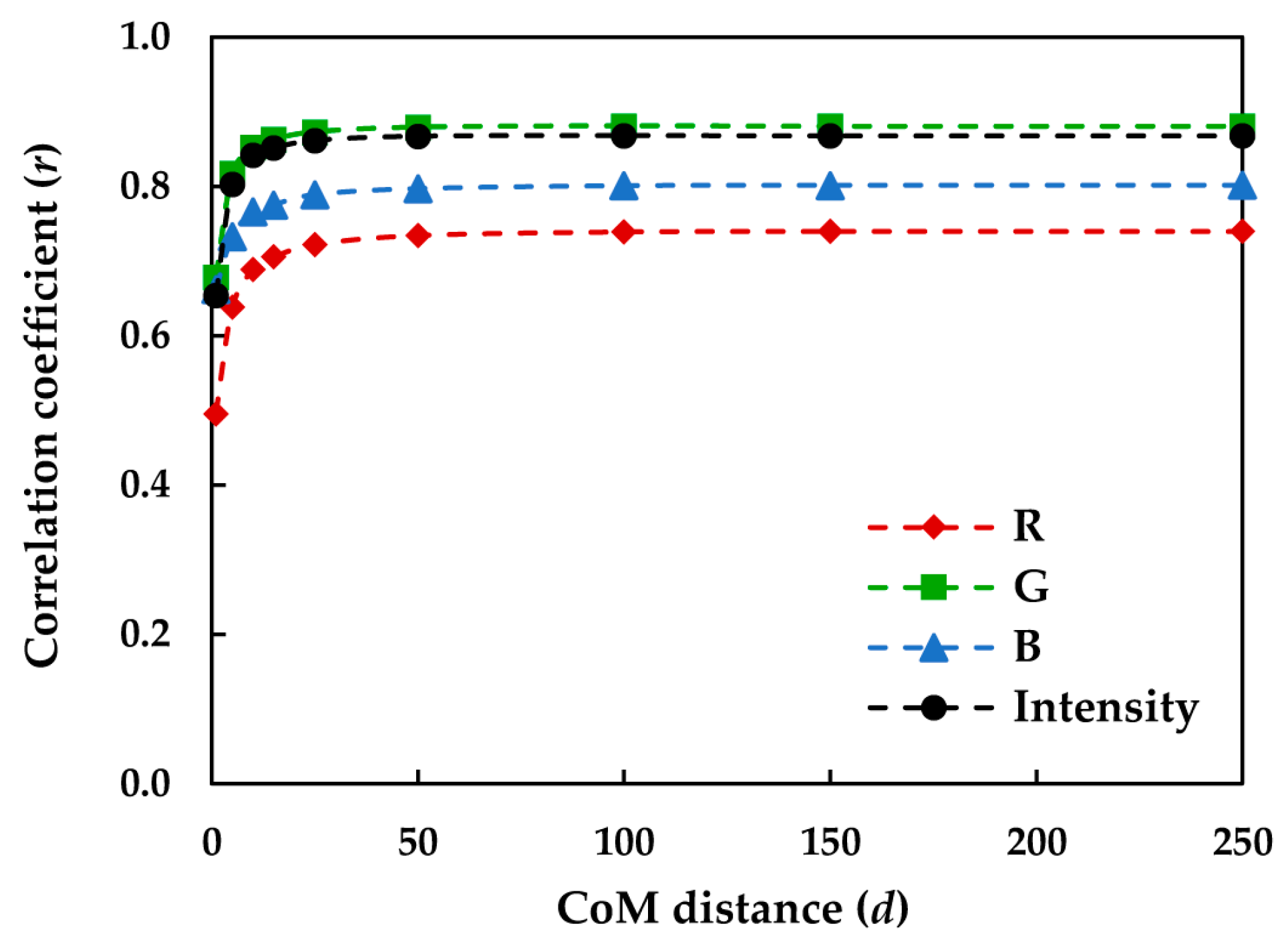
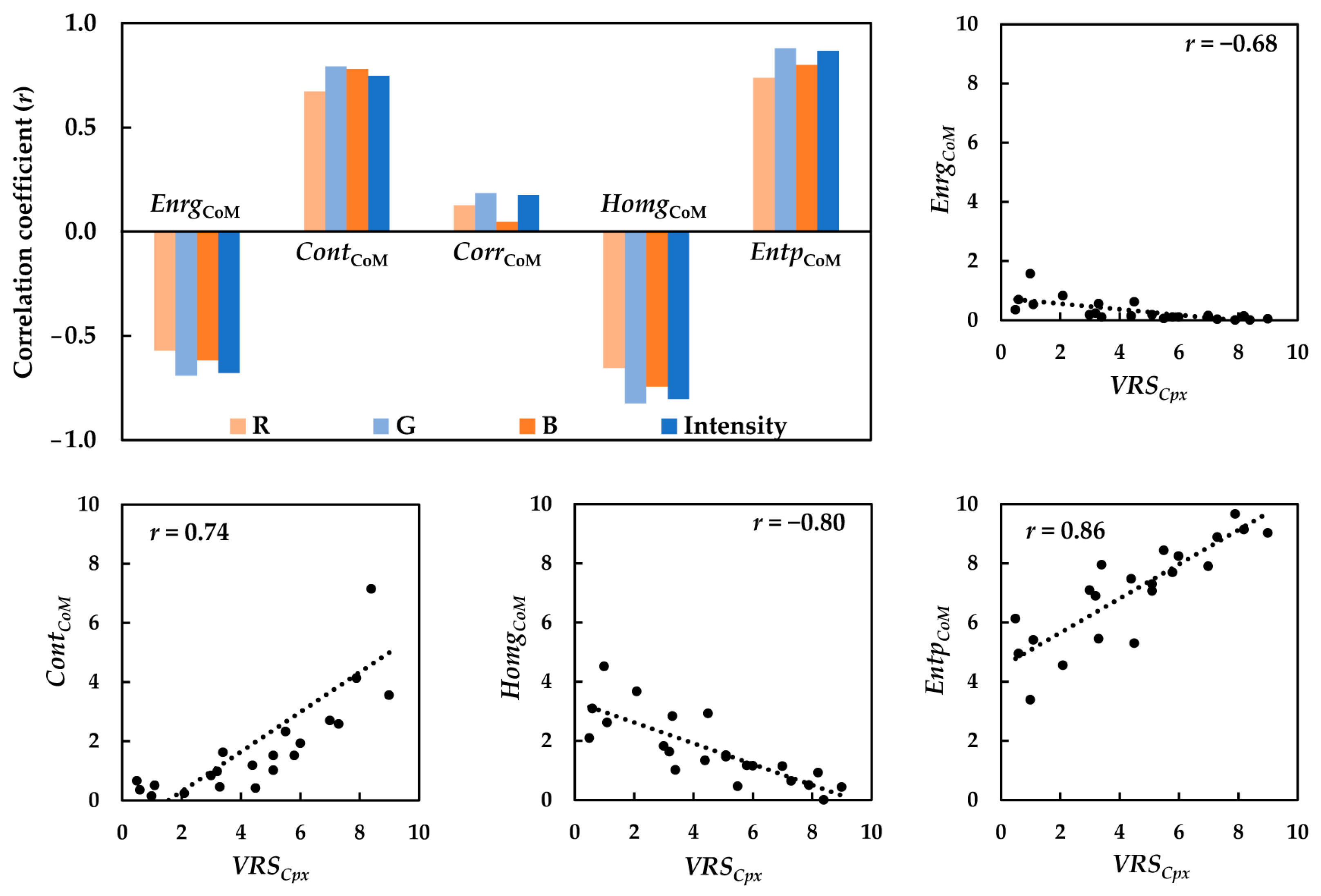
4.3.1. Co-Occurrence Matrix (CoM) Texture Features

Five rotation-invariant CoM features including EnrgCoM, ContCoM, CorrCoM, EntpCoM, and HomgCoM were computed for the textile images the in sRGB, HSV, YCbCr, I1I2I3, and CIELAB color spaces. The relationships between the VRSCpx of the textiles and the corresponding CoM features of the textile images were subsequently determined. Preliminary analysis of the results demonstrated that the correlations depend on the CoM distance (d), in such a way that the correlation improves by increasing d up to the certain value of d = 100 pixels, after which the correlation coefficients (r) remain almost unchanged. Figure 12 shows such a dependency for EntpCoM of the R, G, and B channels and the sRGB intensity images.
Improving the correlations by increasing the CoM distance (d) most likely indicates that for this particular set of image textures, EntpCoM was able to detect the fundamental texture primitives of the images the best when the neighboring pixels were at least 100 pixels apart. This optimal CoM distance (d) is expected to comply with the observers’ field of view during the visual assessment of texture. The field of view is considered as the angle formed within the observer’s eyes with respect to the sample size, particularly, the size of the texture primitives observed on the physical sample. The scanning line of 100 pixels on the image corresponded to a line of 1.5 cm on the physical sample, forming the field of view of approximately 2° at the viewing distance of 40 cm.
The bar graph in Figure 13 compares the five CoM features computed with d = 100 pixels, in terms of their correlations with the visual data. Scatter diagrams of the CoM features with the highest correlation coefficients (r) (i.e., EnrgCoM, HomgCoM ContCoM, and EntpCoM versus the respective visual data) are also depicted in Figure 13. The correlation coefficients (r) in Figure 13 indicate that amongst all of the CoM features, EntpCoM, followed by ContCoM, exhibited the highest positive correlations with VRSCpx, with EntpCoM performing slightly better than ContCoM. HomgCoM and EnrgCoM, on the other hand, had negative correlations with the visual data. Such relationships imply that a texture with higher entropy (or contrast) has lower homogeneity (or energy) and vice versa. Considering the mathematical expressions of these features, such inverse relationships were expected. There seems to be no relationship between CorrCoM and complexity. Again, the highest correlations in the sRGB space belong to the G channel, followed by the sRGB intensity image, and the lowest correlations belong to the R channel.
The CoM features were also computed in the HSV, YCbCr, I1I2I3, and CIELAB color spaces, and their relationships with the VRSCpx of the textiles were evaluated in terms of the correlation coefficient (r). Again, EntpCoM, followed by ContCoM, gave rise to the highest positive correlations with the visual data. The correlation coefficients (r) computed for EntpCoM of the luminance and chrominance channels of the textile images in the five color spaces were compared, as shown in the bar graph in Figure 14.
The correlation analysis in Figure 14 shows the markedly better performance of the luminance channel compared to the chrominance channels, regardless of the color space used. Figure 13 also presents the scatter diagrams of EntpCoM of the images’ luminance channels in HSV, YCbCr, I1I2I3, and CIELAB against the respective visual data. The highest correlation coefficients (r) belonged to the V channel in the HSV, sRGB intensity image, and Y channel in YCbCr. On the other hand, the CIE L* and I1 poorly performed this time.

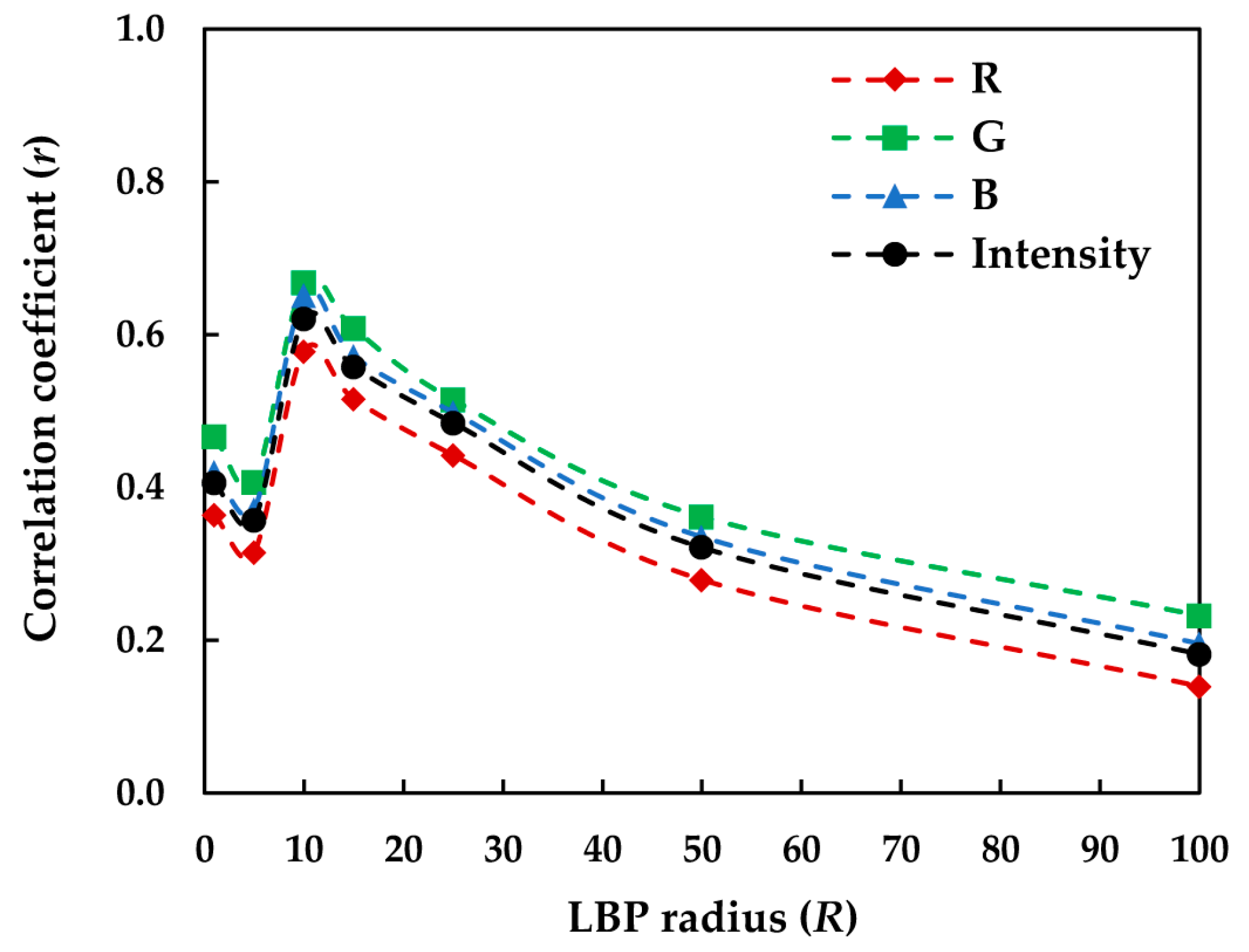
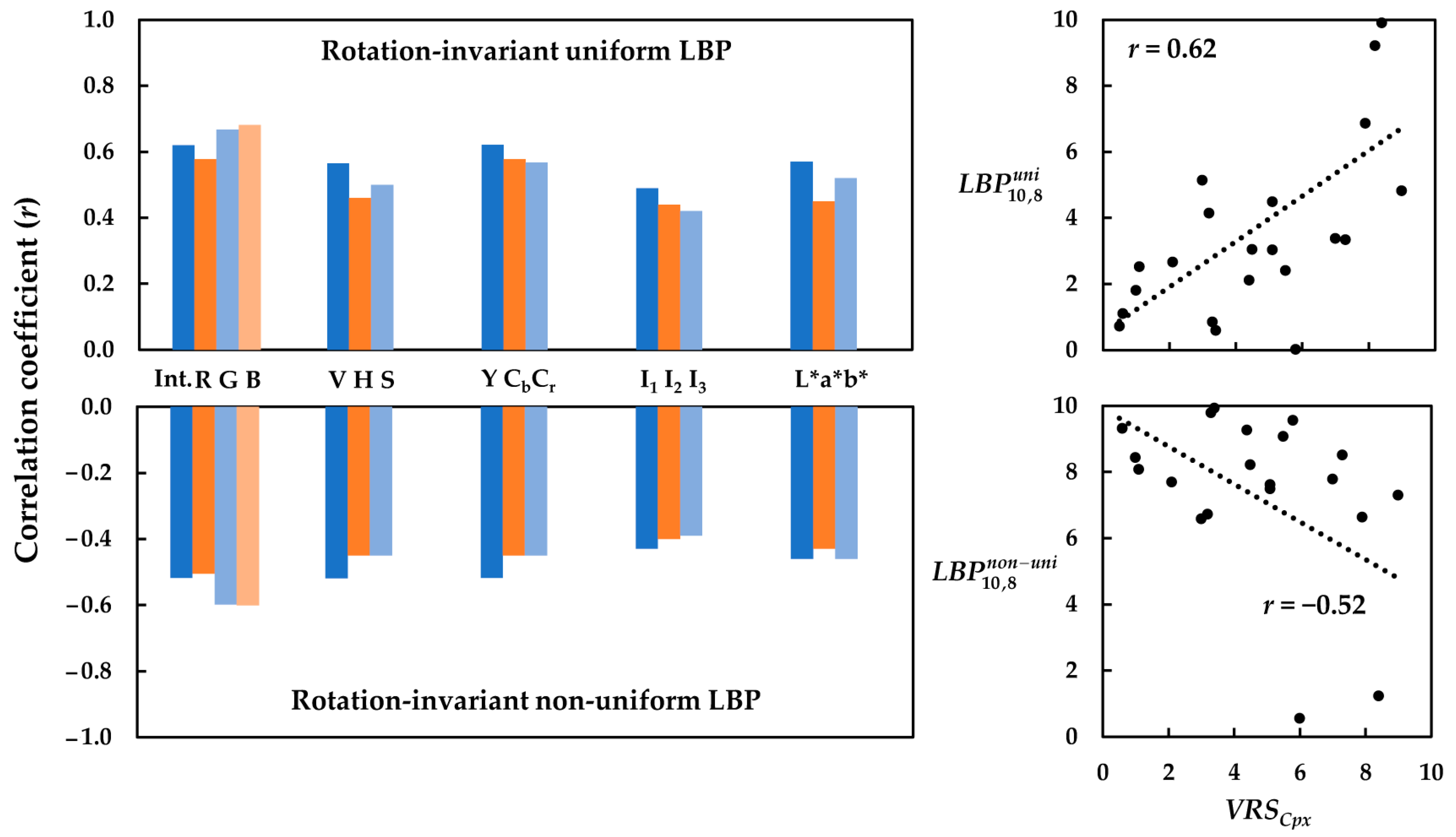
4.3.2. Local Binary Pattern (LBP) Texture Features

As mentioned before, Ojala et al. [54] observed that uniform LBPs were associated with the most fundamental texture primitives present in the image such as bright points, dark points, edges, and corners. For instance, the first pattern in Figure 2b is expected to detect brighter points surrounded by a darker area. Similarly, the ninth pattern could detect darker points embedded in a brighter surrounding. The fourth and sixth patterns could detect corners, while the fifth pattern could detect edges in the texture. The remaining possible patterns were categorized as non-uniform ones.
For N = 8, the LBP histogram for each image texture had ten bins, resulting in a 10 × 1 feature vector, where elements of the vector were frequencies of the respective bins. The first nine bins were associated with the nine uniform LBP patterns (see Figure 2b), and the tenth bin was associated with all non-uniform patterns. The frequencies were linearly re-scaled to be within the range 0–10. We first analyzed the correlation between VRSCpx and each element of the LBP feature vectors in the sRGB space. It was found that the correlation coefficients (r) obtained for the first nine bins were comparatively low, with the first bin having the lowest correlation, and no statistically significant difference between the correlation coefficients (r) of the remaining eight bins (i.e., bins 2–9). Based on these observations, the frequencies of the first nine bins, or the nine uniform LBPs, were determined and averaged for use as the single-number uniform LBP feature. Similarly, the frequency of the tenth bin was determined for use as the non-uniform LBP feature. We assumed that the non-uniform LBP feature could detect non-textured and homogeneous areas in the image texture.
A preliminary analysis of the relationships between the VRSCpx of the textiles and the corresponding LBP features in the sRGB space indicated that the correlations depended on the LBP radius R in such a way that the highest correlations for the uniform LBP feature were obtained when R = 10 pixels. Figure 15 illustrates such dependency for the R, G, and B channels and the sRGB intensity images of the textiles.
These results indicate that for this particular set of image textures, uniform LBPs were able to detect the texture primitives of the images at their best when they scanned the image over circular areas of approximately 20 pixels in diameter. A circular area of approximately 20 pixels in diameter on the image corresponded to a small circular area of approximately 3 mm in diameter on the physical textile sample, forming a field of view of approximately 0.5° at the viewing distance of 40 cm. The respective scanning line on the physical sample for EntpCoM with the CoM distance d = 100 pixels was about 1.5 cm, forming the field of view of approximately 2° at the same viewing distance. This might suggest that uniform LBPs compute the texture in a more localized manner compared to the CoM features.
The high correlation coefficients (r) obtained for EntpCoM suggests that a 2° field of view could reasonably represent the actual observer’s field of view during the visual assessment of texture. On the other hand, the low correlation coefficients (r) obtained for the LBP features indicate that the field of view of 0.5° might not accurately represent the actual observer’s field of view.
Compared to the two previous texture measures (i.e., global σ and EntpCoM, which were successfully tested), the correlation coefficients obtained for the uniform and non-uniform LBP features were low. The bar graphs in Figure 16 compare such correlation coefficients (r) for the relationships between the VRSCpx of the textiles and the corresponding rotation-invariant uniform and non-uniform LBP features with R = 10 pixels and N = 8 neighboring pixels, denoted here as L B P 10 , 8 u n i and L B P 10 , 8 n o n u n i , respectively.
Comparing the correlation coefficients (r) in Figure 16 revealed that uniform and non-uniform LBP features could clearly discriminate between the textile images with more prominent texture patterns and those with a more homogeneous structure. However, the overall correlations were low. Figure 16 also depicts the scatter plots of L B P 10 , 8 u n i and L B P 10 , 8 n o n u n i versus the corresponding VRSCpx of the textiles. L B P 10 , 8 u n i —as the texture measure—had a positive correlation with VRSCpx, while L B P 10 , 8 n o n u n i —as a potential measure for texture homogeneity—was inversely correlated with VRSCpx. Again, the highest correlations belonged to the luminance channels of the images, irrespective of the color space used.

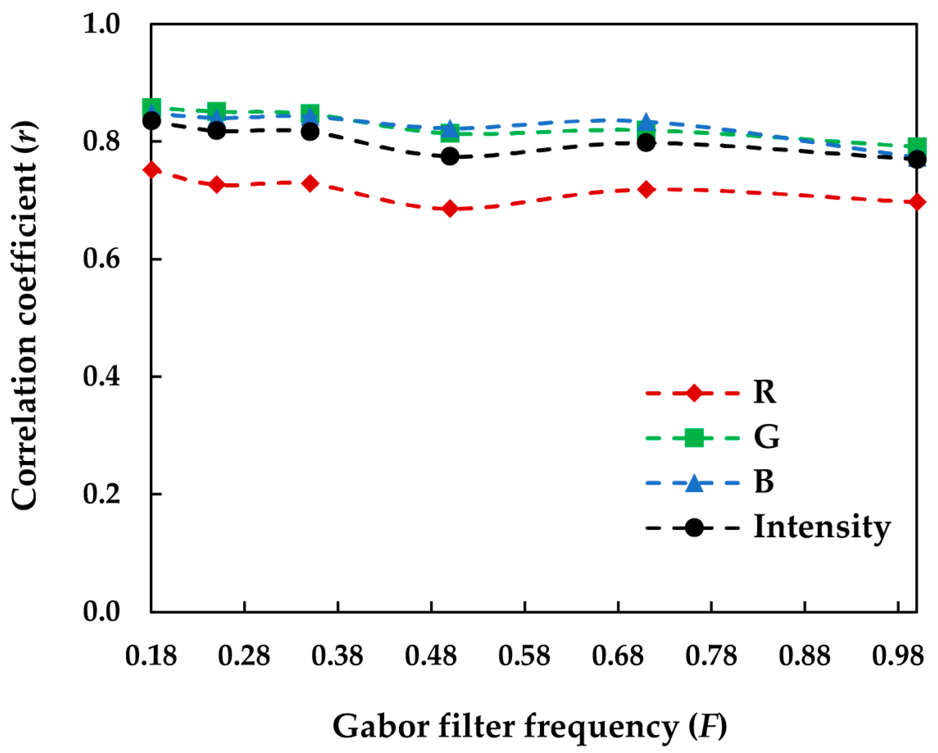
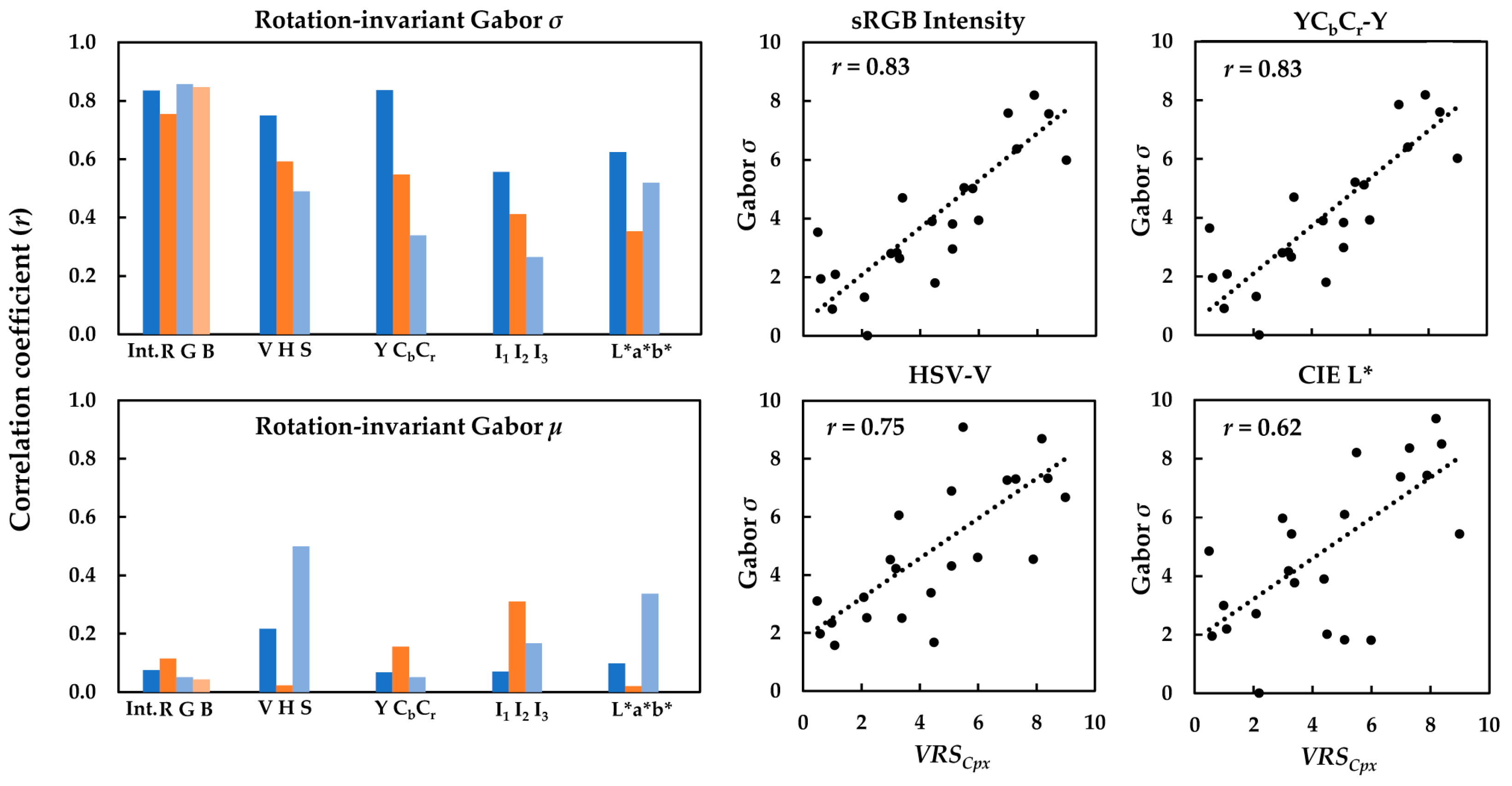
4.3.3. Gabor Features

Rotation-invariant Gabor features (i.e., the mean and standard deviation of the energy of the filtered images, denoted as Gabor µ and Gabor σ, respectively) were computed for the luminance and color channels of the textile images in the sRGB, HSV, YCbCr, I1I2I3, and CIELAB color spaces. The relationships between the VRSCpx of the textiles and Gabor features were then evaluated in terms of the correlation coefficient (r).
To investigate the impact of Gabor filter frequency on such relationships, correlation coefficients (r) for various filter frequencies F were first compared in the sRGB space. It was found that the correlation coefficient (r) tended to generally decline by increasing the filter frequency F in such a way that the highest correlation was achieved for the smallest frequency used to design the Gabor filter bank (i.e., F = 0.18). However, the impact of the filter frequency on the results was quite subtle. Figure 17 illustrates the variation in the correlation coefficient (r) with the filter frequency in the sRGB space.
The very slight changes in the correlation coefficients (r) in Figure 17 indicate that the number of frequencies (nF) chosen to design the Gabor filter bank seems to have had little impact on image texture detection by the filter bank. A similar observation was made by Bianconi and Fernandez [34] for texture classification using Gabor filtering. They demonstrated that the number of frequencies and orientations used to design the filter bank did not significantly affect the accuracy of texture classification.
Given the low impact of the filter frequency on the correlations, Gabor µ and Gabor σ of the textile images computed for F = 0.18 were used for further correlation analysis. The bar graphs in Figure 18 show the correlation coefficients (r) of the relationships between the VRSCpx of the textiles and rotation-invariant Gabor µ and Gabor σ of the luminance and chrominance channels of the textile images in the sRGB, HSV, YCbCr, I1I2I3, and CIELAB color spaces.
A comparison of the correlation coefficients (r) in Figure 18 clearly showed the superiority of Gabor σ in quantifying the visual texture complexity of the textiles compared to Gabor µ. Again, the luminance channels of the images gave rise to stronger relationships between the visual data and computed Gabor σ, regardless of the color space used. Additionally, the highest correlation coefficients (r) belonged to the image luminance channels in sRGB and YCbCr, followed by HSV and CIELAB, while the poorest correlations were obtained in I1I2I3. Scatter plots of the Gabor σ computed for the luminance channel of the textile images against the corresponding VRSCpx of the textiles in these color spaces are also depicted in Figure 18.

5. Discussion

Analyzing the results presented in the previous section helped us to address the three main objectives of this research introduced earlier in the Introduction:

5.1. Perception of Visual Texture Complexity

As mentioned briefly in the previous section, although the textile images employed in this study were color images, the poor relationships between the VRSCpx of the textiles and the texture measures computed for the chrominance channels of the textile images demonstrated that the chrominance channels of the studied luminance–chrominance color spaces poorly performed in quantifying the visual texture complexity. For instance, even though the correlations obtained for the global σ of CIE b* were better than those of CIE a*, both CIE a* and b* performed worse than the luminance channel CIE L*. This indicates that the arrangement of the image texture elements that impacts the observer’s perception of visual texture complexity cannot be represented properly by the CIE a* and b* channels of the images. CIE L*, on the other hand, could represent it markedly better. This also applied to the HSV, YCbCr, and I1I2I3 color spaces. This must be carefully considered when choosing an image channel for quantifying the texture and texture complexity.
Moreover, the good performance of the image luminance channel in the five studied color spaces proved that variations in the luminance of the texture, or as one could call the luminance contrast, plays a crucial role in creating the so-called visual texture complexity. This finding is in agreement with the predictive model proposed in Section 4.1, where visual texture complexity of the textiles was found to be related to the spatial arrangement and spatial frequency of the texture elements, manifested as randomness, strongness, and color variation.
This supports the well-accepted fact that the human visual system interprets the visual signal as separate color and pattern information through separate neural pathways [72]. It also explains why joint color–texture features give rise to worse correlations with the visual data when compared to the correlations obtained for the pure color or pure luminance texture features. In other words, the human visual system is perfectly able to interpret achromatic texture, and color only enriches such interpretations. In this regard, it must be emphasized that typical textile materials usually exhibit lower levels of visual texture complexity compared to textures with a very high dynamic range of spatial frequency such as color fractals. Therefore, a thorough investigation using texture samples with a broad range of texture complexity and color contrast is needed to verify the present results.

5.2. Visual Texture Complexity and Its Correlation with Image Texture Measures

A summary of the performance of the best performing texture measures from different classes investigated in this research (i.e., global σ as an image descriptor and EntpCoM, L B P 10 , 8 u n i , and Gabor σ as texture features in quantifying the visual texture complexity of the textiles) is depicted in Figure 19.
The correlation coefficients (r) in Figure 19 were computed for the luminance channel of the textile images in the sRGB, HSV, YCbCr, I1I2I3, and CIELAB color spaces and exhibited the efficiency of each texture measure and color space in the objective quantification of the visual texture complexity of this particular set of textile samples.
As mentioned before, the global σ measures the spread in the image pixel values. A high global σ indicates an image with high contrast. The high correlation coefficients (r) obtained for the global σ in all five color spaces show that this simple, yet very informative image statistic could be a good candidate for deriving a quantitative measure for the visual texture complexity. Global σ performed the best when computed for the luminance channel of the images, where it provides a measure for the luminance contrast. The main drawback of this image descriptor as a texture measure is its sensitivity to changes in the illumination condition. However, it seems that global σ is much less dependent on the choice of color space compared to other texture features.
EntpCoM reflects the extent to which the pixel values are randomly distributed in the image. Although entropy itself is, by definition, spatially-invariant, the CoM entropy can be computed locally over a range of CoM distances, which makes it a more localized texture detector compared to global σ. EntpCoM exhibited the highest correlations with the visual texture complexity of the textiles in sRGB and YCbCr, with lower correlations in the I1I2I3 and CIELAB color spaces. This indicates that CoM features are more sensitive to changes in the image pixel values and are highly dependent on the choice of color space.
Although uniform and non-uniform LBP features are able to discriminate between the textured and non-textured images, we observed no strong correlation between these features and visual texture complexity of the textiles in this research. This might demonstrate that uniform LBP features are unable to provide sufficient information about the luminance contrast of these image textures.
Gabor filtering is a very powerful tool for a controlled localized extraction of texture information from images by tuning the filter parameters. Some evidence has been provided by the human vision research proving that human brain processes images by a frequency analysis routine [73]. It has also been found that two-dimensional Gabor functions fit the receptive fields of simple cells in the primary visual cortex of mammals [74]. The high correlations between the visual data and the corresponding Gabor σ of the textile images in the present study support such evidence. The correlation coefficients (r) were very close to those of the EntpCoM and global σ in the sRGB and YCbCr color spaces. Moreover, Gabor σ performed better than EntpCoM in the I1I2I3 and CIELAB color spaces. Like EntpCoM, Gabor σ is sensitive to changes in the image pixel values and hence dependent on the choice of color space.
Overall, the results of the correlation analysis demonstrate that a robust texture measure for deriving a quantitative metric for visual texture complexity is one that is able to efficiently detect and quantify the luminance contrast of the texture.
To investigate the joint contribution of the four texture measures to visual texture complexity, a similar generic formula to Equation (2) was used to model the correlation between the VRSCpx and the four computed texture measures for the sRGB intensity images:
V T C p = k 1 [ G l o b a l   σ ] + k 2 [ E n t p C o M ] + k 3 [ L B P 10 , 8 u n i ] + k 4 [ G a b o r   σ ]
where VTCp is again an intermediate variable to hold the predicted visual texture complexity values, and ki, i = 1, 2, …, 4 are coefficients to express the contribution of each texture measure to VTCp. By minimizing the mean squared error (MSE), the best correlation between VRSCpx and VTCp was achieved when k1, k2, k3, and k4 were 0.39, 0.28, 0.03, and 0.30, respectively. These coefficients verify the results of the bivariate correlation analysis in terms of the effectiveness of the global σ, followed by Gabor σ and EntpCoM in quantifying the visual texture complexity.
Considering the higher contributions of global σ and Gabor σ over the others, we performed an exploratory factor analysis [70] on the four texture measures for the sRGB intensity images to evaluate their possible inter-dependencies. The factor loadings/coefficients of the global σ, EntpCoM, L B P 10 , 8 u n i , and Gabor σ for a single common factor analysis, together with their respective specific variances, are presented in Table 2.
The factor loadings in Table 2 show that the single common factor put the most weight on the global σ and Gabor σ. Their corresponding close to zero specific variances indicated that the two measures were almost entirely determined by this common factor. On the other hand, lower weights of L B P 10 , 8 u n i and EntpCoM (and their much higher specific variances) indicated that these two measures were most likely described by other factors. In other words, the global σ and Gabor σ of the image textures in the sRGB space seem to be highly inter-dependent. This explains why both measures showed high correlations with the visual data in the sRGB and YCbCr spaces.

5.3. Most Suitable Color Spaces for Quantitative Evaluation of Visual Texture Complexity

A comparison between the correlation coefficients (r) obtained for various color spaces in Figure 19 revealed that sRGB and YCbCr, followed by HSV, outperformed the I1I2I3 and CIELAB color spaces. YCbCr and HSV were immediate transformations of sRGB: for each image pixel, Y in YCbCr is the weighted sum of the R, G, and B values, and V in HSV is the maximum of the R, G, and B values. Therefore, it appears that for this particular set of image textures, when quantifying the luminance contrast matters, the sRGB space and its transformations (except for I1I2I3) seemed to be more reliable than the uniform color spaces such as CIELAB. I1I2I3 exhibited the worst performance amongst all.
It must be emphasized that although the correlation coefficients (r) obtained for the two chrominance channels of the images were always lower than those of the luminance channel for all five color spaces, one always tended to outperform the others in terms of correlation with the visual data. The best performing chrominance channels were G in sRGB, H in HSV, Cb in YCbCr, I2 in I1I2I3, and b* in CIELAB. This could also be attributed to the dominant blue-green color of the images. In other words, the selection of a suitable color space and color channel for texture quantification tasks is highly influenced by the color characteristics of the image textures.

6. Conclusions

The aim of this research was to investigate how observers interpret the texture complexity of a series of textile fabrics, and the possibility of finding a texture metric to quantify this attribute. The results of the visual assessment experiments revealed that the observers tended to evaluate the texture of the textiles by the aid of several visual cues: homogeneity, randomness, repetitiveness, regularity, color variation, and strongness, and they used these cues to interpret the complexity of texture as a higher-level attribute. We chose to call this attribute the visual texture complexity. Based on the results of the correlation analysis, we could generally define visual texture complexity as the perceived degree of disorder or randomness in the distribution of the color and luminance elements over the surface of a material, which depends on the size, shape, amount, and arrangement of such elements.
To investigate whether there is any potential quantitative metric for visual texture complexity, images of the textiles in the sRGB, HSV, YCbCr, I1I2I3 and CIELAB color spaces were used to compute a number of image statistics and texture features. First-order image statistics, together with co-occurrence matrix, local binary pattern, and Gabor filtering, were chosen as some of the most popular image and texture operators for this purpose. Linear relationships between the ratings of visual texture complexity given by the observers through rank ordering the textiles and the computed features of the textile images were analyzed. Amongst the several first-order image statistics, the standard deviation of the luminance channel of the images showed the highest correlations with the visual data in sRGB, HSV, YCbCr, I1I2I3 and CIELAB color spaces. Additionally, entropy of the co-occurrence matrix and the standard deviation of the image energy after convolving with the Gabor filter, both computed for luminance images in sRGB and YCbCr, showed the highest correlations with the visual data. Such correlations for the uniform LBP features were comparatively low.
The results demonstrate that features that are able to efficiently quantify the image luminance contrast exhibit better correlations with visual texture complexity. The highest correlations were always obtained for the luminance channel of the images, indicating the arrangement of the image texture elements, which impacts the observer’s perception of visual texture complexity, cannot be represented properly by the chrominance channels, particularly for the luminance–chrominance color spaces. Moreover, among the two chrominance channels of the images, one always tended to outperform the other in terms of the correlation with the visual data. This suggests that the choice of a suitable color space and color channel for image texture computation is highly influenced by the color characteristics of the texture database. However, it must be emphasized that these results are strongly associated with the characteristics of the texture database used and might be limited to the tested sample set and experimental conditions. The selected sample set was limited to textile materials that usually exhibit lower levels of visual complexity. Moreover, the number of samples and their texture diversity were limited. Additionally, sRGB and its transformations are considered as device dependent color spaces. Hence, changing the image acquisition device and/or illumination setup could result in different image representations, and therefore different correlations with the visual data. Further research using a more versatile texture database is needed to verify the present results. One could suggest the use of an image-based sample set (instead of physical samples) to verify the findings of the present research.

Author Contributions

Conceptualization, F.M.; methodology, F.M.; software, F.M.; validation, F.M. and J.Y.H.; formal analysis, F.M.; investigation, F.M.; resources, F.M. and J.Y.H.; data curation, F.M.; writing—original draft preparation, F.M.; writing—review and editing, F.M. and J.Y.H.; visualization, F.M.; supervision, J.Y.H.; project administration, J.Y.H.; funding acquisition, J.Y.H. All authors have read and agreed to the published version of the manuscript.

Funding

This work was supported by the Spectraskin project N-288670, funded by the Research Council of Norway, and ERCIM, the European Research Consortium for Informatics and Mathematics through a postdoctoral fellowship.

Institutional Review Board Statement

This study was conducted in accordance with the Nor-wegian Centre for Research Data (NSD) guidelines. Protocol code: 790219, date of approval: 11 January 2021.

Data Availability Statement

HyTexiLa, the dataset of hyperspectral reflectance images can be downloaded from https://color.univ-lille.fr/datasets (accessed on 7 September 2022).

Acknowledgments

The authors wish to thank the anonymous reviewers for their valuable suggestions.

Conflicts of Interest

The authors declare no conflict of interest.

Appendix A. The Written Instruction about the Visual Assessment Experiment

Introduction to Psychophysical Experiment:
This psychophysical experiment is to investigate how human observers perceive the texture of textile materials. According to the International Commission on Illumination, CIE, the appearance of an object can be subdivided into at least four attributes, namely color, gloss, translucency, and texture. This experiment only focuses on texture. To understand better, imagine that you have an old sofa at home. The fabric of the seats is now worn out because of the friction for so many years. You decide to replace the fabric with a new one, so you pick up the phone and call the nearest upholstery fabric producer to see if they have it available in their product line. How would you describe the texture of the fabric to the salesperson in the simplest way so that they can find it for you?
In a previous experiment, we found that observers tend to describe the texture of textiles using the following words/qualities:
  • Homogeneity
  • Randomness
  • Repetitiveness
  • Regularity
  • Color variation
  • Strongness
  • Complexity
In this experiment, we are interested in your understanding of these qualities, and would like to ask you to perform a sorting task on a series of fabrics with respect to these qualities. If you need to check the meaning of any of these words, you can use online dictionaries and then use your own interpretation to perform the experiment.
How to perform the experiment:
This is a rank ordering experiment. A rank ordering experiment is essentially a sorting task. There is a set of 23 textile fabrics. The experimenter will ask you to sit at the table and then present you with all the fabrics. You will have 5 min to familiarize yourself with the samples and evaluate them in terms of their texture. The experimenter will then randomly pick one of the above texture qualities and ask you to sort the fabrics on the table based on how much they represent that quality, from the lowest to the highest. To do the task, you can ask yourself questions like these:
  • How homogeneous is fabric #1?
  • Is there any fabric with higher homogeneity than fabric #1?
After you have finished the sorting, the experimenter will pick the next texture quality and ask you to repeat the sorting. Please avoid leaning forward or backward while sorting to keep your distance from the table.
We deeply thank you for participating in the experiment!

Appendix B. Formulas for Transforming sRGB to HSV, YCbCr, Ohta’s I1I2I3 and CIELAB Color Spaces

Formulas used in this paper to transform the colors in the sRGB space to the corresponding colors in the HSV, YCbCr, Ohta’s I1I2I3 and CIELAB spaces are as follows. In these formulas, R, G, and B denote the red, green, and blue pixel values of the sRGB image, respectively. For an 8-bit sRGB image, R, G, and B are within the range 0–255.

Appendix B.1. sRGB to Intensity Image

Intensity image (I), also known as the grayscale image, is simply the linear transformation of the sRGB image using the weighted sum of the R, G, and B values. The following equation was used to compute the intensity image (I) from the sRGB image [71]:
I = 0.2989 R + 0.5870 G + 0.1140 B

Appendix B.2. sRGB to HSV Color Space

The HSV color space defines colors in terms of three components: hue angle, saturation, and value. Such color components are believed to relate well to human color perception. The hue angle (H) represents a true color such as red, yellow, purple, etc. Saturation (S) and value (V) represent the purity and brightness of the color, respectively. The H, S, and V components of the sRGB image is calculated using the below equations [75]:
H = { 0 i f   T = 0 60 ( G B 255 T mod 6 ) i f   T max = R / 255 60 ( B R 255 T + 2 ) i f   T max = G / 255 60 ( R G 255 T + 4 ) i f   T max = B / 255
S = { 0 i f   T max = 0 T / T max i f   T max 0
V = T max
With
T max = max ( R , G , B ) / 255 T min = min ( R , G , B ) / 255 T = T max T min

Appendix B.3. sRGB to YCbCr Color Space

The YCbCr color space is a widely used standardized color model in digital video processing. It separates the luminance and chrominance components of colors into the luminance component (Y) and the chrominance components blue (Cb) and red (Cr). sRGB images can be transferred into the YCbCr color space using the following linear transformations [71]:
[ Y C b C r ] = [ 16 128 128 ] + [ 65.481 128.553 24.966 37.797 74.203 112 112 93.786 18.214 ] [ R / 255 G / 255 B / 255 ]

Appendix B.4. sRGB to Ohta’s I1I2I3 Color Space

The 111213 color space, proposed by Ohta et al. [76] for color region segmentation, represents colors in terms of three color features I1, I2, and I3, where I1 is the luminance, and I2 and I3 are the chrominance components of the color. The three features can be computed using the following equations [71]:
I 1 = R + G + B 3
I 2 = R B 2
I 3 = 2 G R B 4

Appendix B.5. sRGB to CLELAB Color Space

The CLELAB color space recommended by the international lighting commission CIE in 1976, is a perceptually uniform color space in which color differences perceived by the human visual system correlate well with the Euclidian differences in the color coordinates L*, a*, and b*. CIE L* defines the lightness, and CIE a* and b* represent the redness–greenness, and yellowness–blueness of the color, respectively. In order to transform sRGB images to the CIELAB color space, the R, G, and B values were first converted to intermediate CIEXYZ tristimulus values using the following linear transformations [71]:
[ X Y Z ] = [ 0.412453       0.357580       0.180423 0.212671       0.715160       0.072169 0.019334       0.119193       0.950227 ] [ R G B ]
The CIE L*, a*, and b* color coordinates under a particular illuminant with the tristimulus values XnYnZn are subsequently calculated using the following equations:
L * = 116 f ( Y Y n ) 16
a * = 500 [ f ( X X n ) f ( Y Y n ) ]
b * = 200 [ f ( Y Y n ) f ( Z Z n ) ]
With
f ( U ) = { U 1 3 i f   U > 0.008856 7.787 U + 16 116 i f   U 0.008856

References

  1. Chai, X.J.; Ofen, N.; Jacobs, L.F.; Gabrieli, J.D.E. Scene complexity: Influence on perception, memory, and development in the medial temporal lobe. Front. Hum. Neurosci. 2010, 4, 21. [Google Scholar] [CrossRef] [PubMed]
  2. Bonacci, L.M.; Bressler, S.; Kwasa, J.A.C.; Noyce, A.L.; Shinn-Cunningham, B.G. Effects of visual scene complexity on neural signatures of spatial attention. Front. Hum. Neurosci. 2020, 14, 91. [Google Scholar] [CrossRef] [PubMed]
  3. Sun, Z.; Firestone, C. Curious objects: How visual complexity guides attention and engagement. Cogn. Sci. 2021, 45, e12933. [Google Scholar] [CrossRef] [PubMed]
  4. Van Marlen, T.; van Wermeskerken, M.; van Gog, T. Effects of visual complexity and ambiguity of verbal instructions on target identification. J. Cogn. Psychol. 2018, 31, 206–214. [Google Scholar] [CrossRef]
  5. Cassarino, M.; Setti, A. Complexity as key to designing cognitive-friendly environments for older people. Front. Psychol. 2016, 7, 1329. [Google Scholar] [CrossRef]
  6. Pieters, R.; Wedel, M.; Batra, R. The stopping power of advertising: Measures and effects of visual complexity. J. Mark. 2010, 74, 48–60. [Google Scholar] [CrossRef]
  7. Braun, J.; Amirshahi, S.A.; Denzler, J.; Redies, C. Statistical image properties of print advertisements, visual artworks and images of architecture. Front. Psychol. 2013, 4, 808. [Google Scholar] [CrossRef]
  8. Michailidou, E.; Harper, S.; Bechhofer, S. Visual complexity and aesthetic perception of web pages. In Proceedings of the 26th ACM International Conference on Design of Communication, Lisbon, Portugal, 22–24 September 2008. [Google Scholar]
  9. King, A.J.; Lazard, A.J.; Whit, S.R. The influence of visual complexity on initial user impressions: Testing the persuasive model of web design. Behav. Inform. Technol. 2020, 39, 497–510. [Google Scholar] [CrossRef]
  10. Forsythe, A.; Nadal, M.; Sheehy, N.; Cela-Conde, C.J.; Sawey, M. Predicting beauty: Fractal dimension and visual complexity in art. Br. J. Psychol. 2011, 102, 49–70. [Google Scholar] [CrossRef]
  11. Chen, X.; Li, B.; Liu, Y. The impact of object complexity on visual working memory capacity. Psychology 2017, 8, 929–937. [Google Scholar] [CrossRef] [Green Version]
  12. Madan, C.R.; Bayer, J.; Gamer, M.; Lonsdorf, T.B.; Sommer, T. Visual complexity and affect: Ratings reflect more than meets the eye. Front. Psychol. 2018, 8, 2368. [Google Scholar] [CrossRef] [PubMed]
  13. Kurmi, Y.; Chaurasia, V.; Kapoor, N. Design of a histopathology image segmentation algorithm for CAD of cancer. Optik 2020, 218, 164636. [Google Scholar] [CrossRef]
  14. Bravo, M.J.; Farid, H. Object recognition in dense clutter. Percept. Psychophys. 2006, 68, 911–918. [Google Scholar] [CrossRef] [PubMed]
  15. Ionescu, R.T.; Alexe, B.; Leordeanu, M.; Popescu, M.; Papadopoulos, D.P.; Ferrari, V. How hard can it be? Estimating the difficulty of visual search in an image. In Proceedings of the IEEE Conference on Computer Vision and Pattern Recognition CVPR 2016, Las Vegas, NV, USA, 27–30 June 2016; pp. 2157–2166. [Google Scholar]
  16. Richard, N.; Martínez Ríos, A.; Fernandez-Maloigne, C. Colour local pattern: A texture feature for colour images. J. Int. Colour Assoc. 2016, 16, 56–68. [Google Scholar]
  17. CIE technical committee 8-14: Specification of spatio-chromatic complexity. Available online: https://cie.co.at/technicalcommittees/specification-spatio-chromatic-complexity (accessed on 16 August 2022).
  18. Olivia, A.; Mack, M.L.; Shrestha, M.; Peeper, A. Identifying the perceptual dimensions of visual complexity of scenes. In Proceedings of the 26th Annual Meeting of the Cognitive Science Society, Chicago, IL, USA, 4–7 August 2004; pp. 4–7. [Google Scholar]
  19. Douchová, V. Birkhoff’s aesthetic measure. Acta. U. Carol. Philos. Hist. 2016, 2015, 39–53. [Google Scholar] [CrossRef]
  20. Snodgrass, J.G.; Vanderwart, M. A standardized set of 260 pictures: Norms for name agreement, image agreement, familiarity, and visual complexity. J. Exp. Psychol. 1980, 6, 174–215. [Google Scholar] [CrossRef]
  21. Heaps, C.; Handel, S. Similarity and features of natural textures. J. Exp. Psychol. 1999, 25, 299–320. [Google Scholar] [CrossRef]
  22. Amadasun, M.; King, R. Textural features corresponding to textural properties. IEEE Trans. Syst. Man Cybern. 1989, 19, 1264–1274. [Google Scholar] [CrossRef]
  23. Rao, A.R.; Lohse, G.L. Identifying high level features of texture perception. CVGIP-Graph. Models Image Process. 1993, 55, 218–233. [Google Scholar] [CrossRef]
  24. Mojsilovic, A.; Kovacevic, J.; Kall, D.; Safranek, R.J.; Kicha Ganapathy, S. The vocabulary and grammar of color patterns. IEEE Trans. Image Process. 2000, 9, 417–431. [Google Scholar] [CrossRef]
  25. Guo, X.; Asano, C.M.; Asano, A.; Kurita, T. Visual complexity perception and texture image characteristics. In Proceedings of the International Conference on Biometrics and Kansei Engineering, Takamatsu, Kagawa, Japan, 19–22 September 2011. [Google Scholar]
  26. Ciocca, G.; Corchs, S.; Gasparini, F. Complexity perception of texture images. In New Trends in Image Analysis and Processing–ICIAP 2015 Workshops; Lecture Notes in Computer Science; Murino, V., Puppo, E., Sona, D., Cristani, M., Sansone, C., Eds.; Springer International Publishing: Zürich, Switzerland, 2015; Volume 9281, pp. 119–126. [Google Scholar]
  27. Ciocca, G.; Corchs, S.; Gasparini, F.; Bricolo, E.; Tebano, R. Does color influence image complexity perception? In Computational Color Imaging Workshop, CCIW 2015; Lecture Notes in Computer Science; Trémeau, A., Schettini, R., Tominaga, S., Eds.; Springer: Berlin/Heidelberg, Germany, 2015; Volume 9016, pp. 139–148. [Google Scholar]
  28. Ivanovici, M.; Richard, N. Fractal dimension of color fractal images. IEEE Trans. Image Process. 2011, 20, 227–235. [Google Scholar] [CrossRef] [PubMed]
  29. Brodatz, P. Textures: A Photographic Album for Artists and Designers; Dover Publications: New York, NY, USA, 1996. [Google Scholar]
  30. Nagamachi, M. Kansei Engineering: A new ergonomic consumer-oriented technology for product development. Int. J. Ind. Ergon. 1995, 15, 3–11. [Google Scholar] [CrossRef]
  31. MIT Vision and Modeling Group, Vision Texture. Available online: https://vismod.media.mit.edu/vismod/imagery/VisionTexture/distribution.html (accessed on 16 August 2022).
  32. Haralick, R.M.; Shanmugam, K.; Dinstein, I. Textural features for image classification. IEEE Trans. Syst. Man Cybern. 1973, SMC-3, 610–621. [Google Scholar] [CrossRef]
  33. Ivanovici, M.; Richard, N. A naive complexity measure for color texture images. In Proceedings of the International Symposium on Signals, Circuits and Systems (ISSCS), Iasi, Romania, 13–14 July 2017. [Google Scholar]
  34. Nicolae, I.E.; Ivanovici, M. Color texture image complexity—EEG-sensed human brain perception vs. computed measures. Appl. Sci. 2021, 11, 4306. [Google Scholar] [CrossRef]
  35. Fernandez-Lozano, C.; Carballal, A.; Machado, P.; Santos, A.; Romero, J. Visual complexity modelling based on image features fusion of multiple kernels. PeerJ 2019, 18, e7075. [Google Scholar] [CrossRef] [PubMed]
  36. Mirjalili, F.; Hardeberg, J.Y. Appearance perception of textiles, a tactile and visual study. In Proceedings of the 27th Color Imaging Conference, Paris, France, 21–25 October 2019. [Google Scholar]
  37. Shapiro, L.G.; Stockman, G.C. Computer Vision, 1st ed.; Upper Saddle River; Prentice–Hall: Upper Saddle River, NJ, USA, 2001. [Google Scholar]
  38. Bianconi, F.; Fernández, A.; Smeraldi, F.; Pascoletti, G. Colour and texture descriptors for visual recognition: A historical overview. J. Imaging 2021, 7, 245. [Google Scholar] [CrossRef]
  39. López, F.; Valiente, J.M.; Prats, J.M.; Ferrer, A. Performance evaluation of soft color texture descriptors for surface grading using experimental design and logistic regression. Pattern Recognit. 2008, 41, 1744–1755. [Google Scholar] [CrossRef]
  40. Bianconi, F.; Fernández, A.; Gonzalez, E.; Saetta, S.A. Performance analysis of colour descriptors for parquet sorting. Expert Syst. Appl. 2013, 40, 1636–1644. [Google Scholar] [CrossRef]
  41. Xie, X.; Mirmehdi, M. A galaxy of texture features. In Handbook of Texture Analysis; Mirmehdi, M., Xie, X., Suri, J., Eds.; Imperial College Press: London, UK, 2008; pp. 375–406. [Google Scholar]
  42. Palm, C. Color texture classification by integrative co-occurrence matrices. Pattern Recognit. 2004, 37, 965–976. [Google Scholar] [CrossRef]
  43. Jain, A.; Healey, G. A multiscale representation including opponent color features for texture recognition. IEEE Trans. Image Process. 1998, 7, 124–128. [Google Scholar] [CrossRef]
  44. Bianconi, F.; Harvey, R.W.; Southam, P.; Fernandez, A. Theoretical and experimental comparison of different approaches for color texture classification. J. Electron. Imaging 2011, 20, 43006–430017. [Google Scholar] [CrossRef]
  45. Umbaugh, S.E. Computer Imaging: Digital Image Analysis and Processing; CRC Press: Boca Raton, FL, USA, 2005. [Google Scholar]
  46. Sundararajan, D. Digital Image Processing: A Signal Processing and Algorithmic Approach; Springer: Singapore, 2017. [Google Scholar]
  47. Simone, G.; Pedersen, M.; Hardeberg, J.Y. Measuring perceptual contrast in digital images. J. Vis. Commun. Image Represent. 2012, 23, 491–506. [Google Scholar] [CrossRef]
  48. Albregtsen, F. Statistical Texture Measures Computed from Gray Level Co-Occurrence Matrices. Image Processing Laboratory, Department of Informatics, University of Oslo. 2008. Available online: https://www.uio.no/studier/emner/matnat/ifi/INF4300/h08/undervisningsmateriale/glcm.pdf (accessed on 4 January 2022).
  49. Ou, X.; Pan, W.; Xiao, P. In vivo skin capacitive imaging analysis by using grey level co-occurrence matrix (GLCM). Int. J. Pharm. 2014, 460, 28–32. [Google Scholar] [CrossRef] [PubMed]
  50. Iqbal, N.; Mumtaz, R.; Shafi, U.; Zaidi, S.M.H. Gray level co-occurrence matrix (GLCM) texture based crop classification using low altitude remote sensing platforms. PeerJ Comput. Sci. 2021, 7, e536. [Google Scholar] [CrossRef] [PubMed]
  51. Dhruv, B.; Mittal, N.; Modi, M. Study of Haralick’s and GLCM texture analysis on 3D medical images. Int. J. Neurosci. 2019, 129, 350–362. [Google Scholar] [CrossRef] [PubMed]
  52. Ben Salem, Y.; Nasri, S. Automatic recognition of woven fabrics based on texture and using SVM. Signal Image Video Process. 2010, 4, 429–434. [Google Scholar] [CrossRef]
  53. Gomez, W.; Pereira, W.C.A.; Infantosi, A.F.C. Analysis of co-occurrence texture statistics as a function of gray-level quantization for classifying breast ultrasound. IEEE Trans. Med. Imaging 2012, 31, 1889–1899. [Google Scholar] [CrossRef]
  54. Ojala, T.; Pietikäinen, M.; Mäenpää, T. Multiresolution gray-scale and rotation invariant texture classification with local binary patterns. IEEE Trans. Pattern Anal. 2002, 24, 971–987. [Google Scholar] [CrossRef]
  55. Huang, D.; Shan, C.; Ardabilian, M.; Wang, Y.; Chen, L. Local binary patterns and its application to facial image analysis: A survey. IEEE Trans. Syst. Man Cybern. 2011, 41, 765–781. [Google Scholar] [CrossRef]
  56. Kaya, Y.; Faruk Ertuğrul, Ö.; Tekin, R. Two novel local binary pattern descriptors for texture analysis. Appl. Soft Comput. 2015, 34, 1568–4946. [Google Scholar] [CrossRef]
  57. Bianconi, F.; Fernandez, A. Evaluation of the effects of Gabor filter parameters on texture classification. Pattern Recognit. 2007, 40, 3325–3335. [Google Scholar] [CrossRef] [Green Version]
  58. Mäenpää, T. The Local Binary Pattern Approach to Texture Analysis—Extensions and Applications. Ph.D. Dissertation, Department of Electrical and Information Engineering, University of Oulu, Oulu, Finland, 2003. [Google Scholar]
  59. Cui, C. Comparison of two psychophysical methods for image color quality measurement: Paired comparison and rank order, In Proceedings of the 8th Color Imaging Conference, Scottsdale, AZ, USA, 7–10 November 2000.
  60. Khan, H.A.; Mihoubi, S.; Mathon, B.; Thomas, J.B.; Hardeberg, J.Y. HyTexiLa: High resolution visible and near infrared hyperspectral texture images. Sensors 2018, 18, 2045. [Google Scholar] [CrossRef] [PubMed]
  61. ColorChecker® Classic. Available online: https://www.xrite.com/categories/calibration-profiling/colorchecker-classic (accessed on 1 June 2022).
  62. Thomas, J.B.; Colantoni, P.; Trémeau, A. On the uniform sampling of CIELAB color space and the number of discernible colors. In Computational Color Imaging Workshop, CCIW 2013; Tominaga, S., Schettini, R., Trémeau, A., Eds.; Springer: Berlin/Heidelberg, Germany, 2013; pp. 53–67. [Google Scholar]
  63. Stokman, H.; Gevers, T. Selection and fusion of color models for image feature detection. IEEE Trans. Pattern Anal. Mach. Intell. 2007, 29, 371–381. [Google Scholar] [CrossRef] [PubMed]
  64. Gevers, T.; Gijsenij, A.; van de Weijer, J.; Geusebroek, J.M. Color in Computer Vision: Fundamentals and Applications; John Wiley & Sons: Portland, OR, USA, 2012. [Google Scholar]
  65. Bello-Cerezo, R.; Bianconi, F.; Fernández, A.; González, E.; Di Maria, F. Experimental comparison of color spaces for material classification. J. Electron. Imaging 2016, 25, 61406. [Google Scholar] [CrossRef]
  66. Pachos, G. Perceptually uniform color spaces for color texture analysis: An empirical evaluation. IEEE Trans. Image Process. 2001, 10, 932–937. [Google Scholar] [CrossRef]
  67. Cernadas, E.; Fernández-Delgado, M.; González-Rufino, E.; Carrión, P. Influence of normalization and color space to color texture classification. Pattern Recognit. 2017, 61, 120–138. [Google Scholar] [CrossRef]
  68. Mäenpää, T.; Pietikäinen, M.; Viertola, J. Separating color and pattern information for color texture discrimination. In Proceedings of the 16th International Conference on Pattern Recognition, Montreal, QC, Canada, 11–15 August 2002. [Google Scholar]
  69. García, P.A.; Huertas, R.; Melgosa, M.; Cui, C. Measurement of the relationship between perceived and computed color differences. J. Opt. Soc. Am. A 2007, 24, 1823. [Google Scholar] [CrossRef]
  70. Jolliffe, I.T. PPrincipal Component Analysis and Factor Analysis. In Principal Component Analysis; Springer Series in Statistics; Springer: New York, NY, USA, 1986. [Google Scholar]
  71. Kahu, S.Y.; Raut, R.B.; Bhurchandi, K.M. Review and evaluation of color spaces for image/video compression. Color Res. Appl. 2019, 44, 8–33. [Google Scholar] [CrossRef]
  72. Poirson, B.; Wandell, B. Pattern-color separable pathways predict sensitivity to simple colored patterns. Vision Res. 1996, 34, 515–526. [Google Scholar] [CrossRef]
  73. Daugman, G. Uncertainty relation for resolution in space, spatial frequency and orientation optimized by two-dimensional visual cortical filters. J. Opt. Soc. Am. A 1985, 7, 1160–1169. [Google Scholar] [CrossRef]
  74. Petrou, M.M.P.; Kamata, S. Image Processing: Dealing with Texture, 1st ed.; John Wiley & Sons: Chichester, UK, 2006. [Google Scholar]
  75. Chernov, V.; Alander, J.; Bochko, V. Integer-based accurate conversion between RGB and HSV color spaces. Comput. Electr. Eng. 2015, 46, 328–337. [Google Scholar] [CrossRef]
  76. Ohta, Y.I.; Kanade, T.; Sakai, T. Color information for region segmentation. Comput. Graph. Image Process. 1980, 13, 222–241. [Google Scholar] [CrossRef]
Figure 1. The displacement rules for generating CoMs with the distance d = 1 pixel, and rotation angles θ ∈ {0, 45, 90, 135, 180, 225, 270, 315}° (a). An example of a CoM for [d = 1, θ = 0°] after reducing the image bit depth to n = 8 through quantization (b).
Jimaging 08 00248 g001
Figure 2. An example of generating the decimal LBP code for a pixel using N = 8 neighboring pixels at the radius R = 1 pixel: solid and hollow markers correspond to the pixels with higher and lower values as compared to the central pixel (a). The nine uniform binary patterns used to compute the uniform LBP features using N = 8 neighboring pixels as proposed in [54] (b).
Jimaging 08 00248 g002
Figure 3. Visualizations of the real part of the Gabor function with the frequency F = 0.18 and orientation angles θ ∈ {0, 30, 60, 90, 120, 150}°.
Jimaging 08 00248 g003
Figure 4. Twenty-three textile fabrics used in the rank ordering experiments. Although the sample sizes varied, we made sure that the samples were neither too small nor too large, and each sample enclosed all the essential texture primitives (a). An observer performed the rank ordering experiment, sorting the samples with respect to their perceived texture attribute. This image is reprinted from [36] with permission from IS&T (b). It must be noted that these photographs were taken with a DCLR camera and had undergone JPEG compression for the purpose of showcasing the physical samples versus their digital counterparts. This is why the appearance of the physical samples might seem different from their digital counterparts, which were rendered under standard D65 illumination. The sRGB renderings of the samples are introduced in Section 3.2 and Figure 5.
Jimaging 08 00248 g004
Figure 5. The sRGB images of the 23 textiles used in this research. The images are presented in ascending order in terms of their texture complexity, according to the visual rank scores (VRS) given by the observers. VRSCpx refers to the VRS of complexity. Section 4.1 provides detailed information on how the VRS values were computed.
Jimaging 08 00248 g005
Figure 6. The visual rank scores (VRS) of Tex-19 and Tex-14 for the various texture attributes. For instance, Tex-19 had higher complexity, randomness and strongness, while Tex-14 had higher color variation, regularity, repetitiveness, and homogeneity.
Jimaging 08 00248 g006
Figure 7. The correlation between the VRS of complexity (VRSCpx) and the VRS of homogeneity (VRSH), randomness (VRSR), color variation (VRSCV), strongness (VRSS), regularity (VRSRg), and repetitiveness (VRSRp) for the 23 textiles used in this research.
Jimaging 08 00248 g007
Figure 8. The hypothetical perceptual texture space with visual texture complexity as one of its dimensions.
Jimaging 08 00248 g008
Figure 9. The correlation between VRSCpx and VTCp. VTCp in Equation (2) is an intermediate variable defined to hold the ‘predicted’ visual texture complexity computed as the weighted sum of VRSR, VRSCV, VRSS, VRSRg, and VRSRp to have the best linear correlation with VRSCpx.
Jimaging 08 00248 g009
Figure 10. The correlation between the VRSCpx of the textiles and various image descriptors computed for the R, G, and B channels and the sRGB intensity images of the textiles (left). Scatter plots of the global σ and EntpH versus the corresponding VRSCpx for the sRGB intensity images (right).
Jimaging 08 00248 g010
Figure 11. The correlation between the VRSCpx of the textiles and global σ of the luminance and chrominance channels of the textile images in the sRGB, HSV, YCbCr, I1I2I3 and CIELAB color spaces. Here, ‘Int.’ refers to the sRGB intensity image (top left). Scatter plots of the global σ versus the corresponding VRSCpx for the luminance channel of the textile images in the HSV, YCbCr, I1I2I3, and CIELAB color spaces.
Jimaging 08 00248 g011
Figure 12. The correlation between the VRSCpx of the textiles and EntpCoM of the textile images in the sRGB space improves by increasing the CoM distance (d) up to the certain value of d = 100 pixels, after which the correlation coefficient (r) remains almost unchanged.
Jimaging 08 00248 g012
Figure 13. The correlation between the VRSCpx of the textiles and the CoM features of the textile images computed with the CoM distance d = 100 pixels for the R, G, and B channels and the sRGB intensity images (top left). Scatter plots of EnrgCoM, ContCoM, HomgCoM, and EntpCoM versus the corresponding VRSCpx for the sRGB intensity images.
Jimaging 08 00248 g013
Figure 14. The correlation between the VRSCpx of the textiles and EntpCoM computed for the luminance and chrominance channels of the textile images in the sRGB, HSV, YCbCr, I1I2I3, and CIELAB color spaces with the CoM distance d = 100 pixels. Here, ‘Int.’ refers to the sRGB intensity image (top left). Scatter plots of EntpCoM versus the corresponding VRSCpx for the luminance channel of the textile images in the HSV, YCbCr, I1I2I3, and CIELAB color spaces.
Jimaging 08 00248 g014
Figure 15. The correlation between the VRSCpx of the textiles and rotation-invariant uniform LBP feature of the textile images in the sRGB space depends on the LBP radius R.
Jimaging 08 00248 g015
Figure 16. The correlation between the VRSCpx of the textiles and uniform and non-uniform LBP features computed for the textile images with R = 10 pixels and N = 8 neighboring pixels in the sRGB, HSV, YCbCr, I1I2I3 and CIELAB color spaces. Here, ‘Int.’ refers to sRGB intensity image (left); Scatter plots of uniform and non-uniform LBP features versus the corresponding VRSCpx for the sRGB intensity images (right).
Jimaging 08 00248 g016
Figure 17. The correlation between the VRSCpx of the textiles and rotation-invariant Gabor σ of the textile images in the sRGB space depends very slightly on the Gabor filter frequency (F).
Jimaging 08 00248 g017
Figure 18. The correlation between the VRSCpx of the textiles and the Gabor σ and Gabor µ computed for the luminance and chrominance channels of the textile images with the frequency F = 0.18 in the sRGB, HSV, YCbCr, I1I2I3, and CIELAB color spaces. Here, ‘Int.’ refers to the sRGB intensity image (left). Scatter plots of the Gabor σ versus the corresponding VRSCpx for the luminance channel of the textile images in the sRGB HSV, YCbCr, and CIELAB color spaces (right).
Jimaging 08 00248 g018
Figure 19. The performance of various texture measures computed for the luminance channel of the textile images in the sRGB, HSV, YCbCr, I1I2I3, and CIELAB color spaces in terms of their correlations with the VRSCpx of the textiles given by a panel of observers.
Jimaging 08 00248 g019
Table 1. The results of the PCA on the VRS of the seven visual texture attributes: the first two principal component coefficients, PC1 and PC2.
VariablePC1PC2
VRSH0.44−0.04
VRSR−0.37−0.37
VRSRp−0.080.47
VRSRg0.160.46
VRSCV−0.400.11
VRSS−0.340.05
VRSCpx−0.42−0.15
Table 2. The results of the factor analysis on the computed global σ, EntpCoM, L B P 10 , 8 u n i , and Gabor σ of the sRGB intensity images of the textiles.
Texture MeasureFactor LoadingSpecific Variance
Global σ1.000.01
EntpCoM0.830.32
L B P 10 , 8 u n i 0.640.60
Gabor σ0.960.08
Publisher’s Note: MDPI stays neutral with regard to jurisdictional claims in published maps and institutional affiliations.

