
Review of Turbine Parameterization Models for Large-Eddy Simulation of Wind Turbine Wakes


Abstract
:1. Introduction
2. Fundamentals of Turbine Parameterization Models
2.1. Governing Equations of the Flow Field
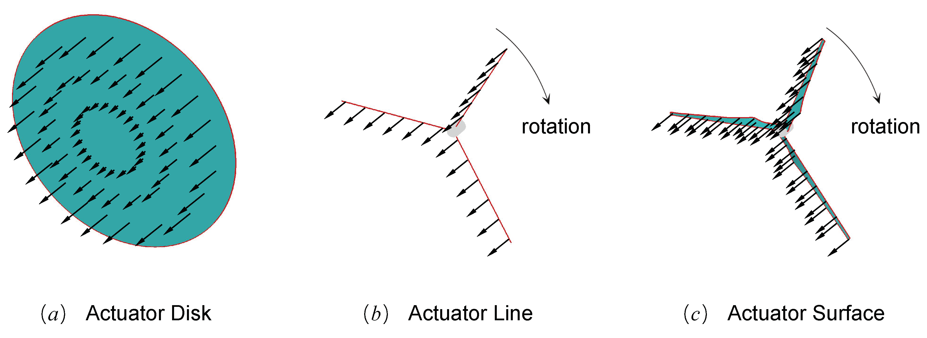
2.2. Actuator Disk Model
2.2.1. Actuator Disk Model with Uniform Thrust
2.2.2. Actuator Disk Model with Non-Uniform Thrust and Tangential Force
2.3. Actuator Line Model
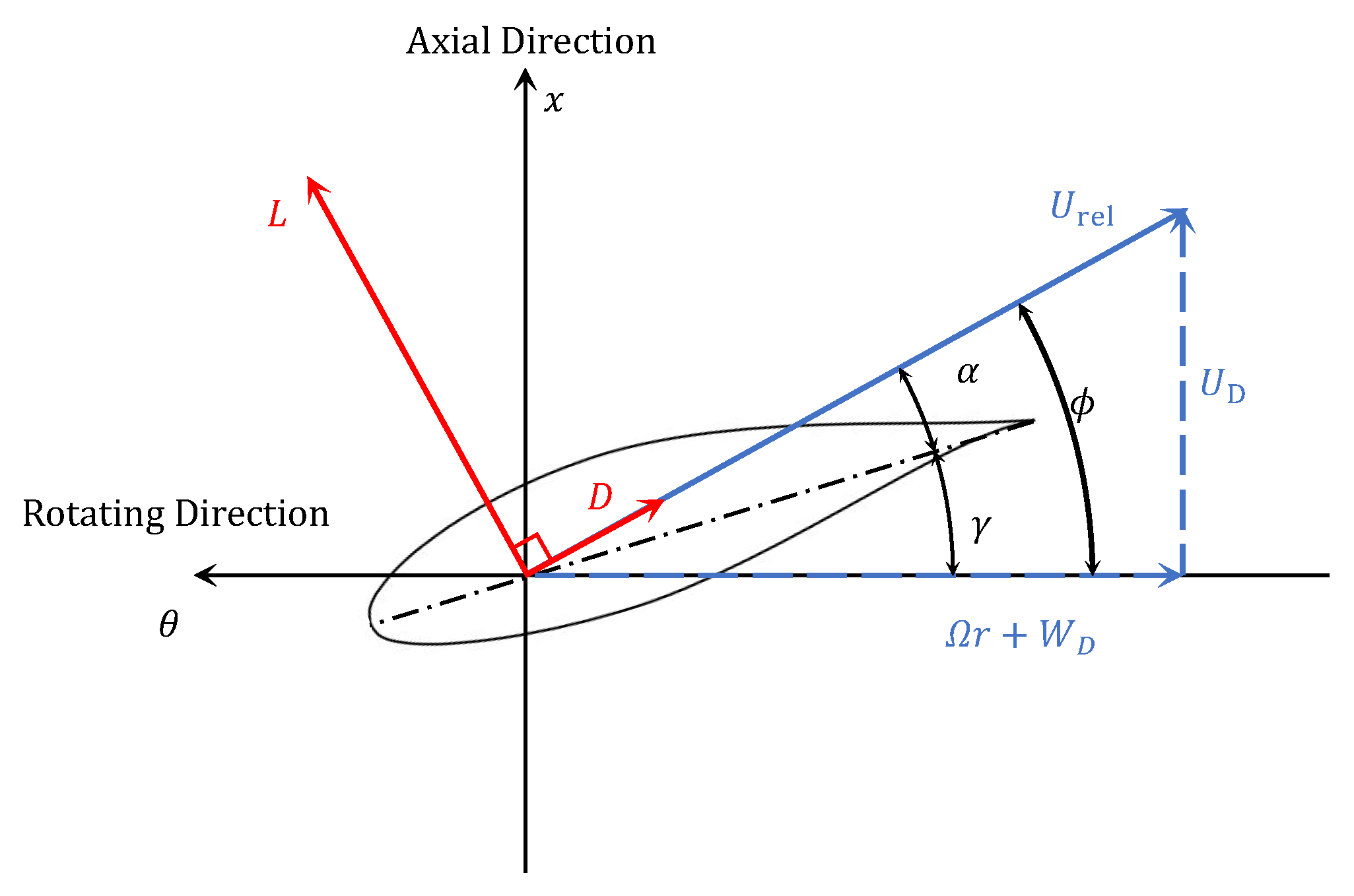
2.3.1. Basic Formulation
2.3.2. Corrections for Three-Dimensional Aerodynamic Effects
2.4. Actuator Surface Model
2.5. Models for Nacelle and Tower
3. Advanced Topics in Wind Turbine Parameterizations
3.1. Distribution of Actuator Forces
3.1.1. Gaussian Distribution
- AD model: The AD model often adopts the 3D isotropic Gaussian distribution for the force distribution, e.g., Sørensen et al. [20], Meyers and Meneveau [23]. Some AD models also adopt the 1D Gaussian distribution (only in the streamwise direction) [28,63]. In general, the force distribution width should be constrained by both rotor diameter D and grid spacing h. Sørensen et al. [20] tested the effect of with an isotropic 3D Gaussian distribution. Their results show that increasing tends to spread the force beyond the disk edge, making the apparent disk larger than its actual size, while a small results in a very sharp transition between the actuator disk and the freestream flow. Thereto, Sørensen and Kock [18], Mikkelsen [63] and Wu and Porté-Agel [27] suggested to set the same as the grid size h.
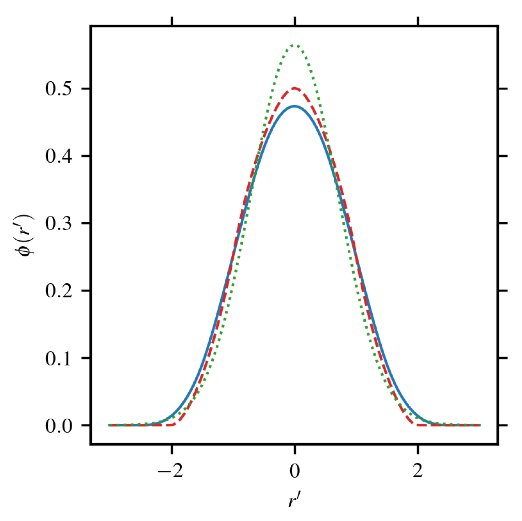
- AL model: Three constraints limit in the AL model, i.e., D, c (the blade chord length) and h. The first constraint, related to D, is imposed mainly to guarantee a correct rotor size for the same reason as the AD model. Martinez et al. [61] found that increasing the smearing length in the AL model also leads to an over-prediction of the turbine power. Martínez-Tossas et al. [64] suggested to use for their cases. The second constraint, imposed by the chord length c, is often more restricted than the first one since the blade is slender for modern wind turbines. From the property of the Gaussian kernel, it is suggested to use so that the force roughly spans from the leading to the trailing edge [6].The results from the work by Martínez-Tossas et al. [65] suggested that using reproduces the flow around a 2D Joukowski airfoil with the best accuracy (see Figure 6). The third constraint, related to the grid size h, is imposed for stability purposes. In the study of Troldborg et al. [62], Troldborg [66], it was found that the Gaussian radius must be set h to avoid spurious oscillations of the blade load and recommended h. More restrict requirement ( h) was also suggested [41]. With the consideration of the force distribution width, Churchfield et al. [6] derived a grid spacing of more than eight grid nodes per chord length near the blade. However, such a requirement implies a very large number of grid nodes and has to be relaxed if the focus is on the far wake evolution [67]. Jha et al. [68] proposed to use an equivalent elliptical wing, whose chord naturally diminishes to zero and to determine the using at each blade section. The authors argued that such a distribution represents better the bounded circulation on the blade. Recently, some dedicated corrections have been proposed for simulations using coarsely resolved AL models, for example, Martínez-Tossas and Meneveau [69] and Meyer Forsting et al. [70]. For non-isotropic projection, setting in the streamwise direction and in the thickness direction results in a more realistic induced velocity field in the 2D airfoil test [65]. Churchfield et al. [55] demonstrated in a 3D AL simulation that the non-isotropic blade force projection results in a more realistic tip vortex, which alleviates the tip load overprediction and reduces the error in the power prediction, even without applying any explicit tip-loss correction.
- AS model: Regarding the AS model, there has not been much discussion on the optimal force distribution. However, since the AS model already spreads the force along the chordwise direction explicitly, one can consider the AS model as a kind of AL model with an idealized chordwise force distribution.
3.1.2. Discrete Delta Function
3.2. Reference Velocity Sampling
3.2.1. Actuator Disk Model
3.2.2. Actuator Line Model
- Collocated single point sampling: This option is adopted by many authors, e.g., Jha et al. [68] and Troldborg et al. [77], because the collation sampling can exclude the induction velocity caused by the lift L at the position of the actuator point. This is because, from the idealized potential flow point of view, the effect of a concentrated lift is equivalent to a bounded circulation. For a smearing lift force using the Gaussian kernel for the distribution, this property is also proved mathematically by Martínez-Tossas et al. [65] and Meyer Forsting et al. [70]. The drag force, on the other hand, induces a non-zero velocity at the collocation point so that the sampled velocity is different from the relative incoming velocity . A relation between and is proposed by Martínez-Tossas et al. [65], as follows,where is the drag coefficient of the airfoil.
- Non-collocated single point sampling: An intuitive choice is to put the velocity sampling point upstream of the actuator point to avoid local induction velocity. However, it is found by Shen et al. [78,79] that the angle of attack is much influenced by the lift induced velocity and proposed to use Biot–Savart law to correct the reference velocity. Similarly, Mittal et al. [42] employed the velocity at the grid node closest to the actuator line point as the reference velocity and also subtracted the lift induced velocity. However, it was found that the single-point sampling method results in fluctuations in the thrust and the power of the rotor.
- Integral sampling: To reduce the fluctuations related to the single point sampling, Churchfield et al. [55] proposed to compute as a weighted-average in a volume close to the actuator point. In their work, the weighting function is the same Gaussian kernel as for the force distribution. The integrated sampling removes spurious high-frequency oscillations effectively. Similarly, the discrete delta function is also employed for computing the reference velocity [54]. A Lagrangian-averaged velocity sampling was proposed by Xie [58], where the reference velocity is computed as the weighted average of velocities sampled sequentially in the time, with the interval adjusted dynamically to the flow patterns to preserve the turbulence information.
3.2.3. Actuator Surface Model
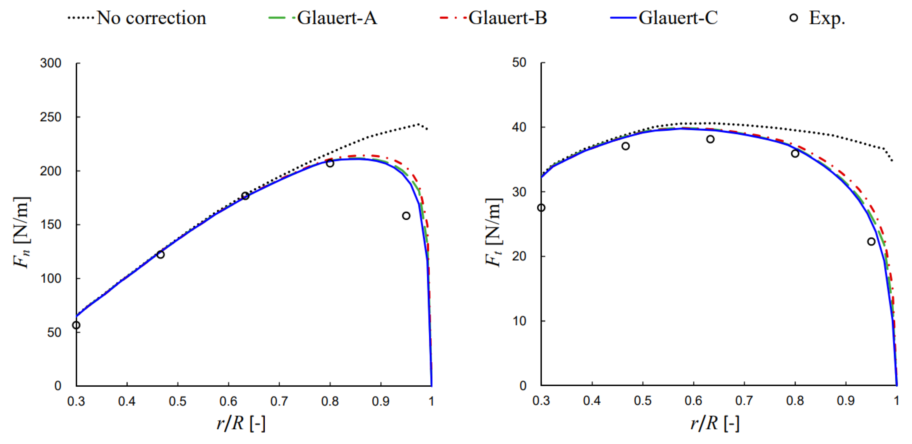
3.3. Tip-Loss Correction
4. Predictive Capability of Wake Characteristics
4.1. Near Wake
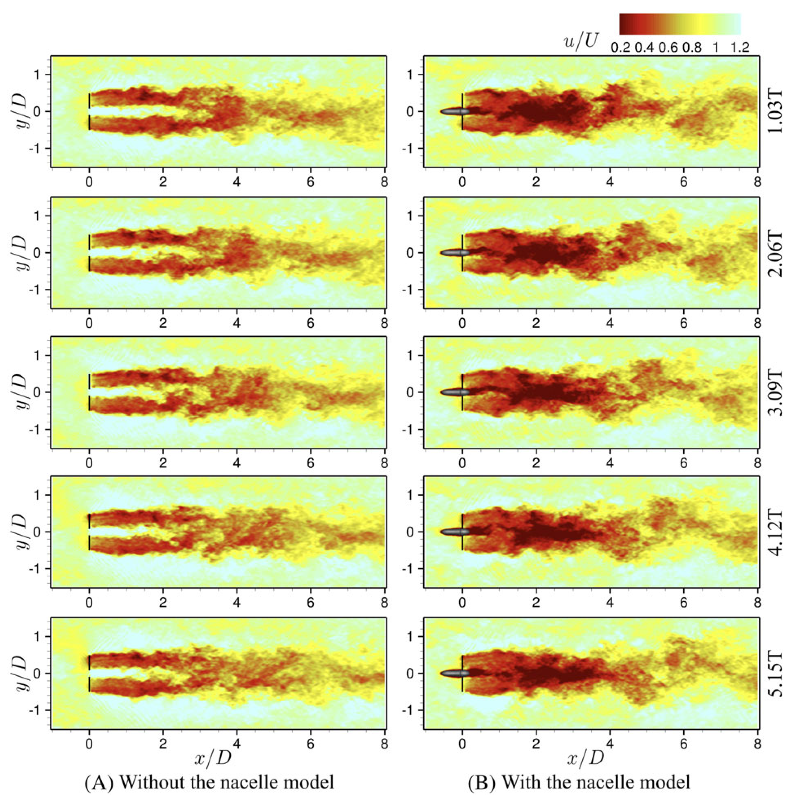
- Mean velocity: The literature agrees that the near wake mean velocity can be predicted very well once the correct radial force distribution is applied. This is naturally achieved by the AL model and the AS model, for which the force distribution is computed from the blade information [10,53,77,98]. For the AD model, accurate near wake velocity can be predicted if the correct radial thrust distribution is provided [77,99], but the tangential force has a negligible effect on the mean streamwise velocity [30]. For an AD model with uniform force distribution, the velocity deficit has a top-hat shape [29,100,101] and persists for approximately downstream for simulations under turbulent inflow [57,100] and for a longer distance (>) under laminar inflow condition [29]. Some special attention should also be paid to the AD model under non-uniform inflow conditions (wind shear/veer or yawed turbine), where the tangential force must be included to capture the wake asymmetry accurately [102,103]. In addition, the nacelle and the tower are critical for predicting the near wake centerline velocity, and thus should be treated properly [10,104].
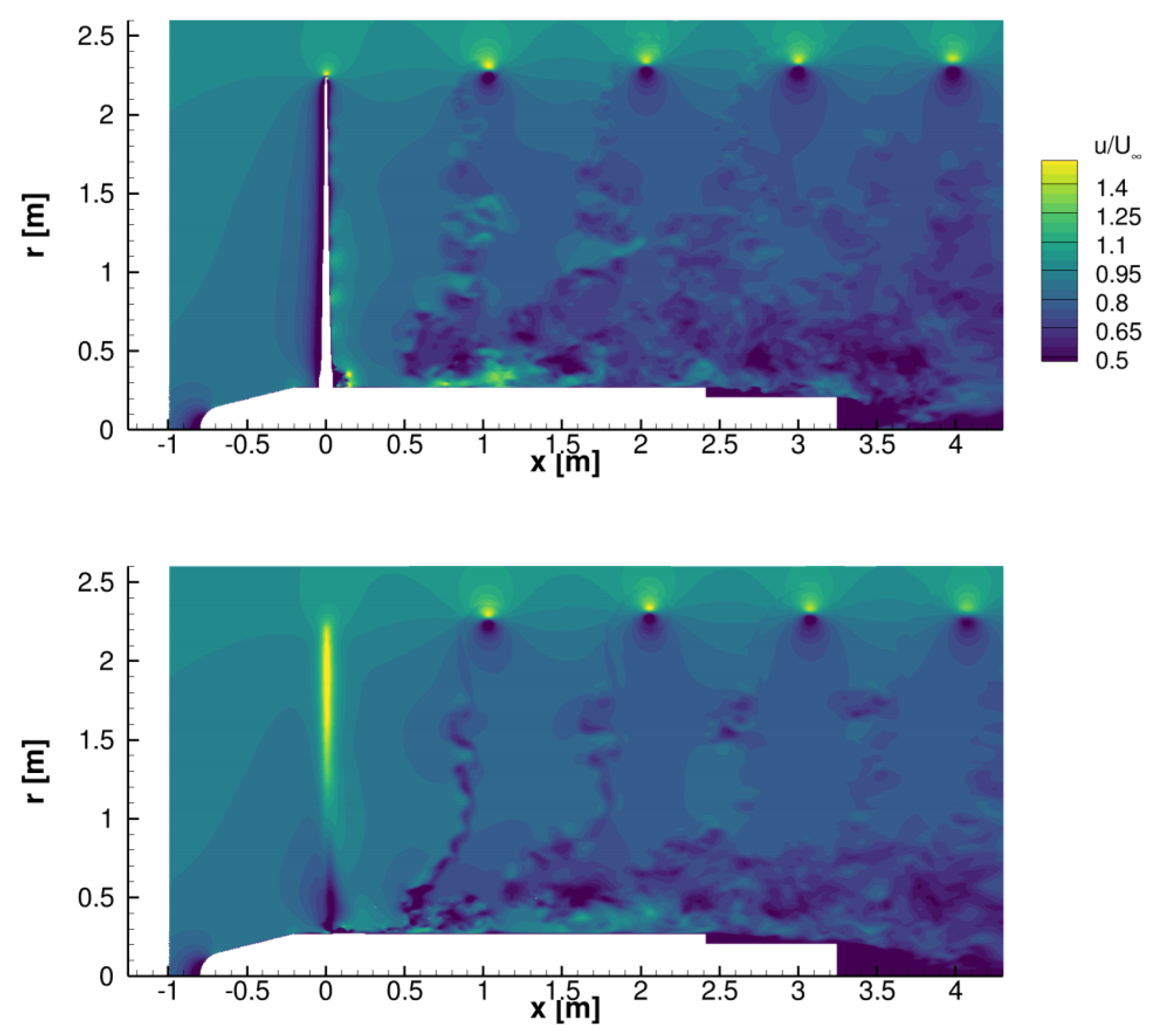
- Turbulence features: Turbulence in the near wake is also heavily dependent on the rotor modeling. Compared with the mean velocity, the prediction of turbulence characteristics by different models is more scattered. Several factors, such as the parameterization models, the numerical discretization, the inflow turbulence, and the tower and nacelle effect, were found to affect the prediction of near-wake turbulence. Results in the literature showed that the parameterization models are prone to underestimate the turbulence intensity, e.g., when compared with the full rotor simulation in Troldborg et al. [53], and the evaluation of the AL model in the blind test workshops organized by Nowitech and Norcowe [89,90,91,92,93,94]. Such an under-prediction is related to unresolved small-scale turbulence structures within the thin shear layer dominated by the tip vortices, which are not captured by the AD model [101,105] or not fully resolved with sufficient accuracy by the AL and AS models (see the discussion following the next bullet). Figure 9 compares the instantaneous flow field predicted by the AL model with that of a geometry resolved simulation [43]. As for the turbulence in the hub region, Yang and Sotiropoulos [10] showed that adding a parameterization for the nacelle improves its prediction when compared with the experimental measurements [97].
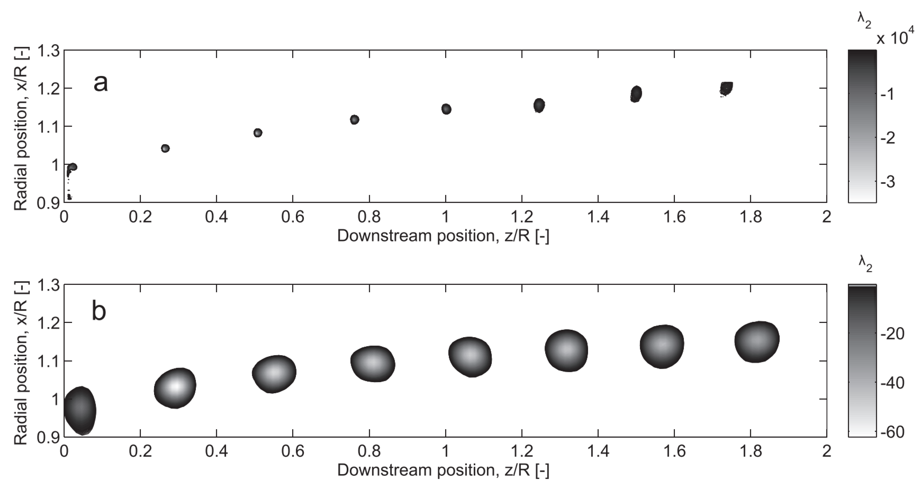
- Tip vortex: One important advantage of the AL and AS models over the AD model is that the tip vortices can be captured thanks to the discrete representation of the blades. The stereo PIV measurement of the near wake of the (new) MEXICO project [82,88] provides a solid database for validating the turbine parameterization models. In general, the literature agrees that the path of the tip vortex is satisfactorily captured in the simulation but the size of the vortex core is not. The simulated vortex cores are often several times larger than those in reality, as shown by Nilsson et al. [106] and Gao et al. [56] and in Figure 10. This overestimation is due to insufficient spatial resolution, although it is already refined to near the tip. A later work of Nathan et al. [98], Nathan [107] also found that a coarse grid with is sufficient to predict the mid-span velocity deficit using the AL model, but resolving the tip vortex core requires extremely fine discretization of . Similar vortex smearing is also observed in Breton et al. [108] using the AS model when comparing with the MEXICO experiment.Albeit the challenge to predict the core size of the tip vortex, the AL model was successfully applied to study the instability of the tip vortices, e.g., Sørensen [109], Ivanell et al. [110], under simple uniform inflows. Ivanell et al. [110] studied the sensitivity of the tip vortices to ambient perturbations (Figure 11). The frequencies triggering the strongest instability are around two peaks close to and (Original definitions were and in Ivanell et al. [110]). Troldborg et al. [62] also found that increasing the tip speed ratio results in an earlier breakdown of tip vortices and transition to turbulence.For the AS model, the predictive capacity for the tip vortices in the near wake of a utility-scale 2.5 MW wind turbine was demonstrated by Yang et al. [111], in which tip vortices with tails and counter-rotating spiral vortices intertwined with the tip vortices, which were observed in the field using the super-large-scale particle image velocimetry (SLPIV) [112], were well predicted.
4.2. Far Wake
- Mean velocity: In general, the literature agrees that it is more challenging to predict the far wake for cases with low inflow turbulence. On one hand, Wang et al. [114] reported a good agreement between the AL predictions and wind tunnel measurements [114]. On the other hand, the AD and AL models are found to underestimate the far wake diffusion compared with the full rotor prediction, even though the mean velocity in the near wake is predicted rather accurately [53]. Another interesting remark is that the AD model (with non-uniform thrust) shows the same level of accuracy when compared with the AL [53,64] and the AS models [30], promoting the use of the AD model for reducing the computational cost. For the cases under turbulent inflow, on the other hand, the mean velocity prediction becomes less dependent on the detail of the rotor so that the AL model [53,114], the AS model [10] and the AD model [100] can accurately predict the mean flow of the wake. Apart from these numerical validations, an interesting experiment investigation was conducted by Aubrun et al. [115,116] in the wind tunnel, which showed that in atmospheric boundary layer turbulence (TI = 0.13), the wakes of a rotor and a porous disk become no longer different beyond three rotor diameters downstream. The effect of nonuniform thrust distribution and rotational force in the AD model is also found not significantly affect the far wake mean velocity (beyond downstream) [27,30,117] using model-to-model comparison.
- Turbulence characteristics: Same as for the mean wake velocity, predicting the turbulence features is also more challenging for cases with low ambient turbulence. Troldborg et al. [53] found that the wake turbulence is under-predicted by the AD and the AL models when compared with the full rotor simulation for cases with low ambient turbulence intensities. For cases with stronger inflow turbulence, the accuracy of the prediction was improved in the above-mentioned works [53,114]. This phenomenon is also supported by the experiment of Aubrun et al. [115,116]. In addition, including the rotation in the AD model is found to improve the accuracy in both uniform and turbulent inflow cases [27,30]. Martinez et al. [61] showed that a large Gaussian projection width can stabilize the wake shear layer and results in smaller TKE in the far wake, under uniform inflow condition.
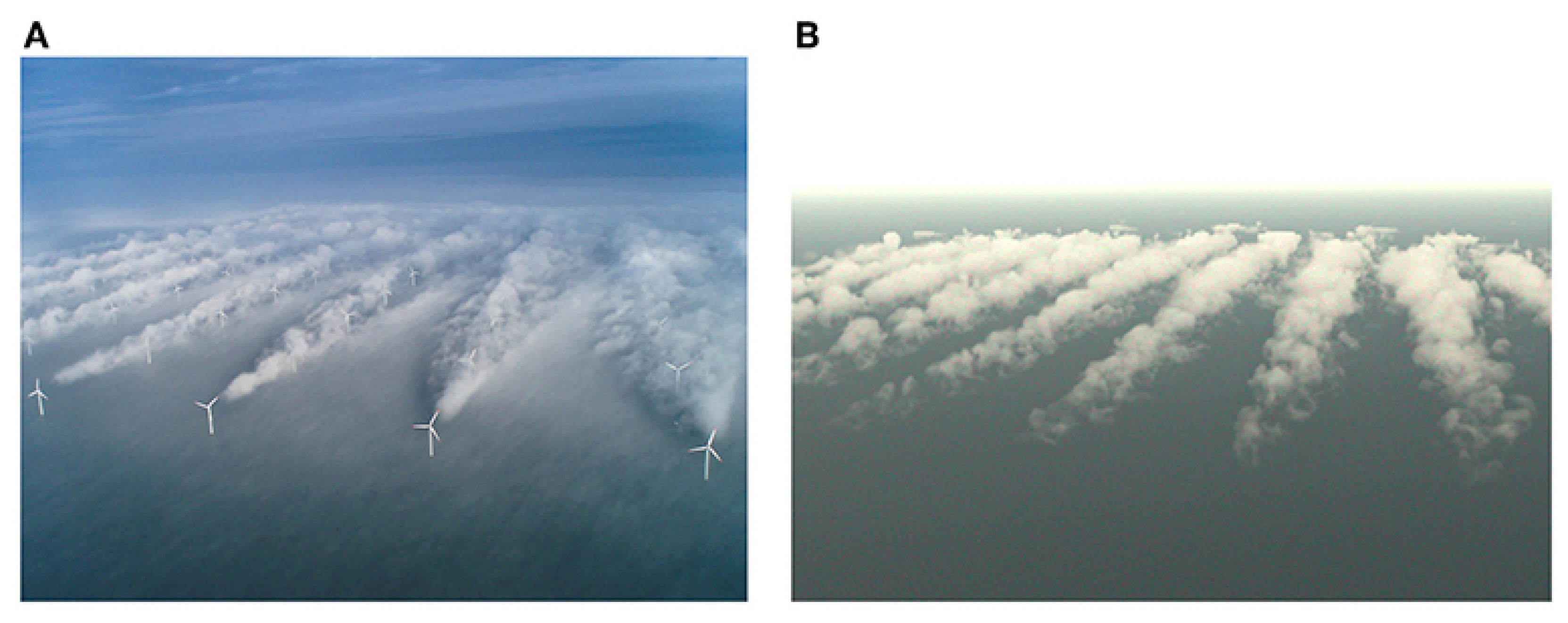
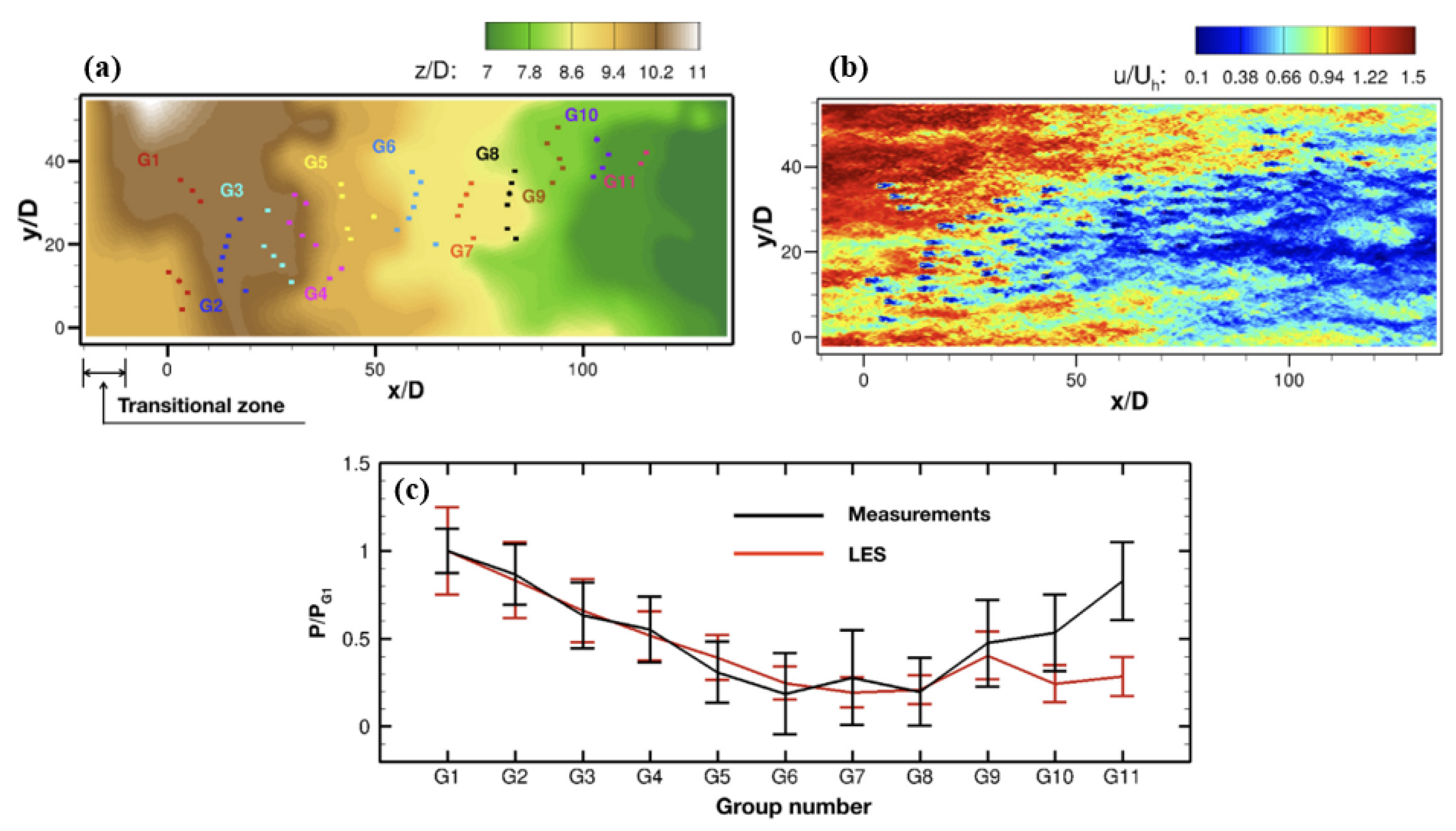
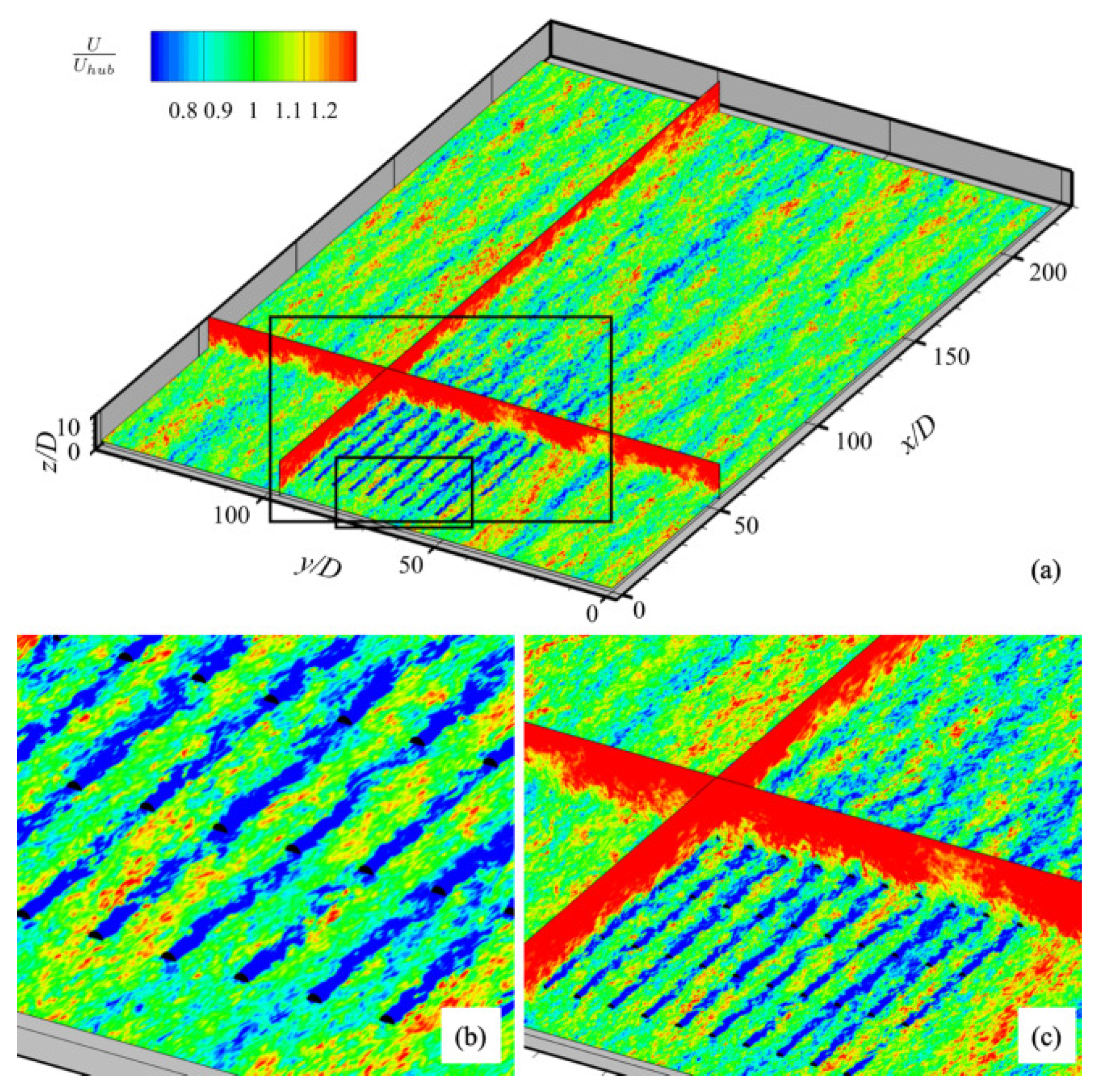
- Large-scale coherent structures: The most important dynamic feature in the far wake is the low frequency, large amplitude wake meandering. These large-scale coherent structures have gained a lot of attention in wind energy research, as they are crucial for wake recovery and dynamic loads on downwind turbines [118]. A recent review on wake meandering can be found in the paper by Yang and Sotiropoulos [119]. Hence, it is important to verify how well these coherent structures can be predicted by the turbine parameterization models. Kang et al. [46] compared the predictions from the AL and AD models with those from the geometry-resolved simulations and found that both models underpredict the turbulence kinetic energy and the wake meandering. Yang and Sotiropoulos [10] showed that using the AS models for blades and nacelle can accurately predict the wake meandering, when compared with the measurements. Compared with the AS/AL models, the spatial and temporal resolutions are lower for the AD model. For simulations of wind farms with large spatial and temporal scales, the AD model is preferred because of its computational efficiency. It is important to systematically evaluate the capability of the AD model in predicting large-scale coherent structures. Li and Yang [29] analyzed the coherent structures in the wake predicted by the AD model (uniform thrust) by comparing its predictions with the AS model. The dynamic mode decomposition (DMD) analyses reveal distinct coherent structures for the wake predicted by the AD model and the AS model in terms of both the dominant frequencies and spatial patterns of different DMD modes as shown in Figure 12 for the case under uniform inflow.In a recent work by Dong et al. [30], it was found that the capability of the AD model in predicting the turbulence kinetic energy in the far wake depends on turbine designs. For a rotor with a relatively uniform axial force coefficient, the turbulence kinetic energy predicted by the AD model is similar to those predicted by the AS model. When the axial force coefficient has a strong radial variation, i.e., lower near the tip but higher near the root, the wake meandering is underpredicted by the AD model than the AS model does, also resulting in lower turbulence kinetic energy for the AD model prediction.The wind turbine parameterization models were successfully applied to study the mechanism of wake meandering. For instance, the far wake meandering triggered by the shear layer instability of the wake was investigated by Mao and Sørensen [120] using the AD model and Gupta and Wan [121] using the AL model. For a floating offshore wind turbine, Li et al. [50] found that small-amplitude turbine’s side-to-side motion () of certain frequencies () can trigger far wake meandering of high amplitude (), by using the AS simulations. Moreover, Li et al. [50] also showed that both uniform and non-uniform AD models with the AS nacelle model are able to capture such instability. Using the AS simulations, Yang and Sotiropoulos [122] showed the co-existence of the inflow large eddy mechanism and the shear layer instability mechanism for wake meandering.
5. Applications to Utility-Scale Wind Farms
6. Summary
Author Contributions
Funding
Institutional Review Board Statement
Informed Consent Statement
Data Availability Statement
Conflicts of Interest
References
- Barthelmie, R.J.; Hansen, K.S.; Frandsen, S.T.; Rathmann, O.; Schepers, J.G.; Schlez, W.; Phillips, J.; Rados, K.; Zervos, A.; Politis, E.S.; et al. Modelling and measuring flow and wind turbine wakes in large wind farms offshore. Wind Energy 2009, 12, 431–444. [Google Scholar] [CrossRef]
- Thomsen, K.; Sørensen, P. Fatigue loads for wind turbines operating in wakes. J. Wind Eng. Ind. Aerodyn. 1999, 80, 121–136. [Google Scholar] [CrossRef]
- Stevens, R.; Meneveau, C. Flow structure and turbulence in wind farms. Annu. Rev. Fluid Mech. 2017, 49, 311–339. [Google Scholar] [CrossRef]
- Porté-Agel, F.; Bastankhah, M.; Shamsoddin, S. Wind-turbine and wind-farm flows: A review. Bound.-Layer Meteorol. 2020, 174, 1–59. [Google Scholar] [CrossRef] [PubMed]
- Sanderse, B.; Van der Pijl, S.; Koren, B. Review of computational fluid dynamics for wind turbine wake aerodynamics. Wind Energy 2011, 14, 799–819. [Google Scholar] [CrossRef]
- Churchfield, M.; Lee, S.; Moriarty, P.; Martinez, L.; Leonardi, S.; Vijayakumar, G.; Brasseur, J. A large-eddy simulation of wind-plant aerodynamics. In Proceedings of the 50th AIAA Aerospace Sciences Meeting Including the New Horizons Forum and Aerospace Exposition, Nashville, TN, USA, 9–12 January 2012; p. 537. [Google Scholar]
- Batten, W.M.; Harrison, M.; Bahaj, A. Accuracy of the actuator disc-RANS approach for predicting the performance and wake of tidal turbines. Philos. Trans. R. Soc. A Math. Phys. Eng. Sci. 2013, 371, 20120293. [Google Scholar] [CrossRef]
- Sørensen, J.N.; Shen, W.Z. Numerical modeling of wind turbine wakes. J. Fluids Eng. Trans. ASME 2002, 124, 393–399. [Google Scholar] [CrossRef]
- Shen, W.Z.; Zhang, J.H.; Sørensen, J.N. The actuator surface model: A new Navier–Stokes based model for rotor computations. J. Sol. Energy Eng. 2009, 131. [Google Scholar] [CrossRef]
- Yang, X.; Sotiropoulos, F. A new class of actuator surface models for wind turbines. Wind Energy 2018, 21, 285–302. [Google Scholar] [CrossRef]
- Germano, M.; Piomelli, U.; Moin, P.; Cabot, W.H. A dynamic subgrid-scale eddy viscosity model. Phys. Fluids A Fluid Dyn. 1991, 3, 1760–1765. [Google Scholar] [CrossRef] [Green Version]
- Froude, R.E. On the part played in propulsion by differences of fluid pressure. In TRANSACTIONS of the Institution of Naval Architects; Institution of Naval Architects: London, UK, 1889; Volume 30, pp. 390–405. [Google Scholar]
- Betz, A. Das Maximum der theoretisch möglichen Ausnutzung des Windes durch Windmotoren. Z. Gesamte Turbinenwesten 1920, 20, 307–309. [Google Scholar]
- Betz, A. The maximum of the theoretically possible exploitation of wind by means of a wind motor. Wind Eng. 2013, 37, 441–446. [Google Scholar] [CrossRef]
- Glauert, H. The Analysis of Experimental Results in the Windmill Brake and Vortex Ring States of an Airscrew; HM Stationery Office: Richmond, UK, 1926. [Google Scholar]
- Conway, J.T. Analytical solutions for the actuator disk with variable radial distribution of load. J. Fluid Mech. 1995, 297, 327–355. [Google Scholar] [CrossRef]
- Conway, J.T. Exact actuator disk solutions for non-uniform heavy loading and slipstream contraction. J. Fluid Mech. 1998, 365, 235–267. [Google Scholar] [CrossRef]
- Sørensen, J.N.; Kock, C.W. A model for unsteady rotor aerodynamics. J. Wind Eng. Ind. Aerodyn. 1995, 58, 259–275. [Google Scholar] [CrossRef]
- Sørensen, J.N.; Myken, A. Unsteady actuator disc model for horizontal axis wind turbines. J. Wind Eng. Ind. Aerodyn. 1992, 39, 139–149. [Google Scholar] [CrossRef]
- Sørensen, J.; Shen, W.; Munduate, X. Analysis of wake states by a full-field actuator disc model. Wind Energy: Int. J. Prog. Appl. Wind Power Convers. Technol. 1998, 1, 73–88. [Google Scholar] [CrossRef]
- Ammara, I.; Leclerc, C.; Masson, C. A viscous three-dimensional differential/actuator-disk method for the aerodynamic analysis of wind farms. J. Sol. Energy Eng. 2002, 124, 345–356. [Google Scholar] [CrossRef]
- Jimenez, A.; Crespo, A.; Migoya, E.; Garcia, J. Advances in large-eddy simulation of a wind turbine wake. J. Phys. Conf. Ser. 2007, 75, 012041. [Google Scholar] [CrossRef]
- Meyers, J.; Meneveau, C. Large eddy simulations of large wind-turbine arrays in the atmospheric boundary layer. In Proceedings of the 48th AIAA Aerospace Sciences Meeting Including the New Horizons Forum and Aerospace Exposition, Orlando, FL, USA, 4–7 January 2010; p. 827. [Google Scholar]
- Calaf, M.; Meneveau, C.; Meyers, J. Large eddy simulation study of fully developed wind-turbine array boundary layers. Phys. Fluids 2010, 22, 015110. [Google Scholar] [CrossRef]
- Calaf, M.; Parlange, M.B.; Meneveau, C. Large eddy simulation study of scalar transport in fully developed wind-turbine array boundary layers. Phys. Fluids 2011, 23, 126603. [Google Scholar] [CrossRef] [Green Version]
- Glauert, H. Airplane propellers. In Aerodynamic Theory; Springer: Berlin/Heidelberg, Germany, 1935; pp. 169–360. [Google Scholar]
- Wu, Y.T.; Porté-Agel, F. Large-Eddy Simulation of Wind-Turbine Wakes: Evaluation of Turbine Parametrisations. Bound.-Layer Meteorol. 2011, 138, 345–366. [Google Scholar] [CrossRef]
- Sørensen, J.N.; Nilsson, K.; Ivanell, S.; Asmuth, H.; Mikkelsen, R.F. Analytical body forces in numerical actuator disc model of wind turbines. Renew. Energy 2020, 147, 2259–2271. [Google Scholar] [CrossRef]
- Li, Z.; Yang, X. Evaluation of actuator disk model relative to actuator surface model for predicting utility-scale wind turbine wakes. Energies 2020, 13, 3574. [Google Scholar] [CrossRef]
- Dong, G.; Li, Z.; Qin, J.; Yang, X. Predictive capability of actuator disk models for wakes of different wind turbine designs. Renew. Energy 2022, 188, 269–281. [Google Scholar] [CrossRef]
- Froude, W. The Elementary Relation between Pitch, Slip, and Propulsive Efficiency. In TRANSACTIONS of the Institution of Naval Architects; Institution of Naval Architects: London, UK, 1878; Volume 19, pp. 22–33. [Google Scholar]
- Schreck, S.; Robinson, M. Rotational augmentation of horizontal axis wind turbine blade aerodynamic response. Wind Energy Int. J. Prog. Appl. Wind Power Convers. Technol. 2002, 5, 133–150. [Google Scholar]
- Shen, W.Z.; Mikkelsen, R.; Sørensen, J.N.; Bak, C. Tip loss corrections for wind turbine computations. Wind Energy 2005, 8, 457–475. [Google Scholar] [CrossRef]
- Du, Z.; Selig, M. A 3-D stall-delay model for horizontal axis wind turbine performance prediction. In Proceedings of the 1998 ASME Wind Energy Symposium, Reno, NV, USA, 12–15 January 1998; p. 21. [Google Scholar]
- Chaviaropoulos, P.; Hansen, M.O. Investigating three-dimensional and rotational effects on wind turbine blades by means of a quasi-3D Navier-Stokes solver. J. Fluids Eng. 2000, 122, 330–336. [Google Scholar] [CrossRef]
- Dobrev, I.; Massouh, F.; Rapin, M. Actuator surface hybrid model. J. Phys. Conf. Ser. 2007, 75, 012019. [Google Scholar] [CrossRef]
- Sibuet Watters, C.; Breton, S.P.; Masson, C. Application of the actuator surface concept to wind turbine rotor aerodynamics. Wind Energy 2010, 13, 433–447. [Google Scholar] [CrossRef]
- Kim, T.; Oh, S.; Yee, K. Improved actuator surface method for wind turbine application. Renew. Energy 2015, 76, 16–26. [Google Scholar] [CrossRef]
- Shen, W.Z.; Sørensen, J.N.; Zhang, J. Actuator surface model for wind turbine flow computations. In Proceedings of the European Wind Energy Conference and Exhibition, Milan, Italy, 7–10 May 2007; Volume 7. [Google Scholar]
- Foti, D.; Yang, X.; Shen, L.; Sotiropoulos, F. Effect of wind turbine nacelle on turbine wake dynamics in large wind farms. J. Fluid Mech. 2019, 869, 1–26. [Google Scholar] [CrossRef]
- Shives, M.; Crawford, C. Mesh and load distribution requirements for actuator line CFD simulations. Wind Energy 2013, 16, 1183–1196. [Google Scholar] [CrossRef]
- Mittal, A.; Sreenivas, K.; Taylor, L.K.; Hereth, L. Improvements to the actuator line modeling for wind turbines. In Proceedings of the 33rd Wind Energy Symposium, Kissimmee, FL, USA, 5–9 January 2015; p. 0216. [Google Scholar]
- Cormier, M.; Weihing, P.; Lutz, T. Evaluation of the Effects of Actuator Line Force Smearing on Wind Turbines Near-Wake Development. J. Phys. Conf. Ser. 2021, 1934, 012013. [Google Scholar] [CrossRef]
- Abraham, A.; Dasari, T.; Hong, J. Effect of turbine nacelle and tower on the near wake of a utility-scale wind turbine. J. Wind Eng. Ind. Aerodyn. 2019, 193, 103981. [Google Scholar] [CrossRef]
- Santoni, C.; Carrasquillo, K.; Arenas-Navarro, I.; Leonardi, S. Effect of tower and nacelle on the flow past a wind turbine. Wind Energy 2017, 20, 1927–1939. [Google Scholar] [CrossRef]
- Kang, S.; Yang, X.; Sotiropoulos, F. On the onset of wake meandering for an axial flow turbine in a turbulent open channel flow. J. Fluid Mech. 2014, 744, 376–403. [Google Scholar] [CrossRef]
- Foti, D.; Yang, X.; Guala, M.; Sotiropoulos, F. Wake meandering statistics of a model wind turbine: Insights gained by large eddy simulations. Phys. Rev. Fluids 2016, 1, 044407. [Google Scholar] [CrossRef]
- Churchfield, M.J.; Lee, S.; Schmitz, S.; Wang, Z. Modeling wind turbine tower and nacelle effects within an actuator line model. In Proceedings of the 33rd Wind Energy Symposium, Kissimmee, FL, USA, 5–9 January 2015; p. 0214. [Google Scholar]
- Sotiropoulos, F.; Yang, X. Immersed boundary methods for simulating fluid–structure interaction. Prog. Aerosp. Sci. 2014, 65, 1–21. [Google Scholar] [CrossRef]
- Li, Z.; Dong, G.; Yang, X. Onset of wake meandering for a floating offshore wind turbine under side-to-side motion. J. Fluid Mech. 2022, 934, A29. [Google Scholar] [CrossRef]
- Li, Z.; Yang, X. Large-eddy simulation on the similarity between wakes of wind turbines with different yaw angles. J. Fluid Mech. 2021, 921, A11. [Google Scholar] [CrossRef]
- Liu, X.; Li, Z.; Yang, X.; Xu, D.; Kang, S.; Khosronejad, A. Large-Eddy Simulation of Wakes of Waked Wind Turbines. Energies 2022, 15, 2899. [Google Scholar] [CrossRef]
- Troldborg, N.; Zahle, F.; Réthoré, P.E.; Sørensen, N. Comparison of the wake of different types of wind turbine CFD models. In Proceedings of the 50th AIAA Aerospace Sciences Meeting including the New Horizons Forum and Aerospace Exposition, Nashville, TN, USA, 9–12 January 2012; p. 237. [Google Scholar]
- Yang, X.; Sotiropoulos, F.; Conzemius, R.J.; Wachtler, J.N.; Strong, M.B. Large-eddy simulation of turbulent flow past wind turbines/farms: The Virtual Wind Simulator (VWiS). Wind Energy 2015, 18, 2025–2045. [Google Scholar] [CrossRef]
- Churchfield, M.J.; Schreck, S.J.; Martinez, L.A.; Meneveau, C.; Spalart, P.R. An advanced actuator line method for wind energy applications and beyond. In Proceedings of the 35th Wind Energy Symposium, Grapevine, TX, USA, 9–13 January 2017; p. 1998. [Google Scholar]
- Gao, Z.; Li, Y.; Wang, T.; Ke, S.; Li, D. Recent improvements of actuator line-large-eddy simulation method for wind turbine wakes. Appl. Math. Mech. 2021, 42, 511–526. [Google Scholar] [CrossRef]
- Yang, X.; Sotiropoulos, F. On the predictive capabilities of LES-actuator disk model in simulating turbulence past wind turbines and farms. In Proceedings of the 2013 American Control Conference, Washington, DC, USA, 17–19 June 2013; pp. 2878–2883. [Google Scholar]
- Xie, S. An actuator-line model with Lagrangian-averaged velocity sampling and piecewise projection for wind turbine simulations. Wind Energy 2021, 24, 1095–1106. [Google Scholar] [CrossRef]
- Réthoré, P.E.; Sørensen, N.N. A discrete force allocation algorithm for modelling wind turbines in computational fluid dynamics. Wind Energy 2012, 15, 915–926. [Google Scholar] [CrossRef]
- Troldborg, N.; Sørensen, N.N.; Réthoré, P.E.; van der Laan, M. A consistent method for finite volume discretization of body forces on collocated grids applied to flow through an actuator disk. Comput. Fluids 2015, 119, 197–203. [Google Scholar] [CrossRef]
- Martinez, L.; Leonardi, S.; Churchfield, M.; Moriarty, P. A comparison of actuator disk and actuator line wind turbine models and best practices for their use. In Proceedings of the 50th AIAA Aerospace Sciences Meeting including the New Horizons Forum and Aerospace Exposition, Nashville, TN, USA, 9–12 January 2012; p. 900. [Google Scholar]
- Troldborg, N.; Sørensen, J.N.; Mikkelsen, R. Numerical simulations of wake characteristics of a wind turbine in uniform inflow. Wind Energy 2010, 13, 86–99. [Google Scholar] [CrossRef]
- Mikkelsen, R. Actuator Disc Methods Applied to Wind Turbines. Ph.D. Thesis, Technical University of Denmark, Lyngby, Denmark, 2003. [Google Scholar]
- Martínez-Tossas, L.A.; Churchfield, M.J.; Leonardi, S. Large eddy simulations of the flow past wind turbines: Actuator line and disk modeling. Wind Energy 2015, 18, 1047–1060. [Google Scholar] [CrossRef]
- Martínez-Tossas, L.A.; Churchfield, M.J.; Meneveau, C. Optimal smoothing length scale for actuator line models of wind turbine blades based on Gaussian body force distribution. Wind Energy 2017, 20, 1083–1096. [Google Scholar] [CrossRef]
- Troldborg, N. Actuator Line Modeling of Wind Turbine Wakes. Ph.D. Thesis, Technical University of Denmark, Lyngby, Denmark, 2009. [Google Scholar]
- Martinez-Tossas, L.A.; Churchfield, M.J.; Yilmaz, A.E.; Sarlak, H.; Johnson, P.L.; Sørensen, J.N.; Meyers, J.; Meneveau, C. Comparison of four large-eddy simulation research codes and effects of model coefficient and inflow turbulence in actuator-line-based wind turbine modeling. J. Renew. Sustain. Energy 2018, 10, 033301. [Google Scholar] [CrossRef]
- Jha, P.; Churchfield, M.; Moriarty, P.; Schmitz, S. Guidelines for Volume Force Distributions Within Actuator Line Modeling of Wind Turbines on Large-Eddy Simulation-Type Grids. J. Sol. Energy Eng. 2014, 136, 031003. [Google Scholar] [CrossRef]
- Martínez-Tossas, L.A.; Meneveau, C. Filtered lifting line theory and application to the actuator line model. J. Fluid Mech. 2019, 863, 269–292. [Google Scholar] [CrossRef]
- Meyer Forsting, A.R.; Pirrung, G.R.; Ramos-García, N. A vortex-based tip/smearing correction for the actuator line. Wind Energy Sci. 2019, 4, 369–383. [Google Scholar] [CrossRef]
- Peskin, C.S. The immersed boundary method. Acta Numer. 2002, 11, 479–517. [Google Scholar] [CrossRef]
- Yang, X.; Zhang, X.; Li, Z.; He, G.W. A smoothing technique for discrete delta functions with application to immersed boundary method in moving boundary simulations. J. Comput. Phys. 2009, 228, 7821–7836. [Google Scholar] [CrossRef]
- Yang, X.; Kang, S.; Sotiropoulos, F. Computational study and modeling of turbine spacing effects in infinite aligned wind farms. Phys. Fluids 2012, 24, 115107. [Google Scholar] [CrossRef]
- Schepers, J.; Schreck, S. Aerodynamic measurements on wind turbines. Wiley Interdiscip. Rev. Energy Environ. 2019, 8, e320. [Google Scholar] [CrossRef]
- Politis, E.S.; Prospathopoulos, J.; Cabezon, D.; Hansen, K.S.; Chaviaropoulos, P.; Barthelmie, R.J. Modeling wake effects in large wind farms in complex terrain: The problem, the methods and the issues. Wind Energy 2012, 15, 161–182. [Google Scholar] [CrossRef]
- Shapiro, C.R.; Gayme, D.F.; Meneveau, C. Filtered actuator disks: Theory and application to wind turbine models in large eddy simulation. Wind Energy 2019, 22, 1414–1420. [Google Scholar] [CrossRef]
- Troldborg, N.; Zahle, F.; Réthoré, P.E.; Sørensen, N.N. Comparison of wind turbine wake properties in non-sheared inflow predicted by different computational fluid dynamics rotor models. Wind Energy 2015, 18, 1239–1250. [Google Scholar] [CrossRef]
- Shen, W.Z.; Hansen, M.O.; Sørensen, J.N. Determination of the angle of attack on rotor blades. Wind Energy 2009, 12, 91–98. [Google Scholar] [CrossRef]
- Shen, W.Z.; Hansen, M.O.; Sørensen, J.N. Determination of angle of attack (AOA) for rotating blades. In Wind Energy; Springer: New York, NY, USA, 2007; pp. 205–209. [Google Scholar]
- Ramdin, S. Prandtl Tip Loss Factor Assessed. Master’s Thesis, Delft University of Technology, Delft, The Netherlands, 2017. [Google Scholar]
- Zhong, W.; Wang, T.G.; Zhu, W.J.; Shen, W.Z. Evaluation of tip loss corrections to AD/NS simulations of wind turbine aerodynamic performance. Appl. Sci. 2019, 9, 4919. [Google Scholar] [CrossRef]
- Snel, H.; Schepers, J.; Montgomerie, B. The MEXICO project (Model Experiments in Controlled Conditions): The database and first results of data processing and interpretation. J. Phys. Conf. Ser. 2007, 75, 012014. [Google Scholar] [CrossRef]
- Schepers, J.; Boorsma, K.; Cho, T.; Gomez-Iradi, S.; Schaffarczyk, P.; Jeromin, A.; Lutz, T.; Meister, K.; Stoevesandt, B.; Schreck, S.; et al. Mexnet (Phase 1): Analysis of Mexico Wind Tunnel measurements. In Proceedings of the Final Report of IEA Task 29; IEA: Paris, France, 2012. [Google Scholar]
- Shen, W.Z.; Zhu, W.J.; Sørensen, J.N. Actuator line/Navier–Stokes computations for the MEXICO rotor: Comparison with detailed measurements. Wind Energy 2012, 15, 811–825. [Google Scholar] [CrossRef]
- Shen, W.Z.; Zhu, W.J.; Yang, H. Validation of the Actuator Line Model for Simulating Flows Past Yawed Wind Turbine Rotors. J. Power Energy Eng. 2015, 03, 7–13. [Google Scholar] [CrossRef]
- Stanly, R.; Martínez-Tossas, L.A.; Frankel, S.H.; Delorme, Y. Large-Eddy Simulation of a wind turbine using a Filtered Actuator Line Model. J. Wind Eng. Ind. Aerodyn. 2022, 222, 104868. [Google Scholar] [CrossRef]
- Boorsma, K.; Schepers, J. New MEXICO experiment. In Preliminary Overview with Initial Validation; Technical Report ECN-E–14-048; ECN: Petten, The Netherland, 2014. [Google Scholar]
- Boorsma, K.; Schepers, J. Rotor experiments in controlled conditions continued: New Mexico. J. Phys. Conf. Ser. 2016, 753, 022004. [Google Scholar] [CrossRef]
- Krogstad, P.Å.; Sætran, L. Wind turbine wake interactions; results from blind tests. J. Phys. Conf. Ser. 2015, 625, 012043. [Google Scholar] [CrossRef]
- Krogstad, P.Å.; Eriksen, P.E. “Blind test” calculations of the performance and wake development for a model wind turbine. Renew. Energy 2013, 50, 325–333. [Google Scholar] [CrossRef]
- Pierella, F.; Krogstad, P.Å.; Sætran, L. Blind Test 2 calculations for two in-line model wind turbines where the downstream turbine operates at various rotational speeds. Renew. Energy 2014, 70, 62–77. [Google Scholar] [CrossRef]
- Krogstad, P.Å.; Sætran, L.; Adaramola, M.S. “Blind Test 3” calculations of the performance and wake development behind two in-line and offset model wind turbines. J. Fluids Struct. 2015, 52, 65–80. [Google Scholar] [CrossRef]
- Bartl, J.; Sætran, L. Blind test comparison of the performance and wake flow between two in-line wind turbines exposed to different turbulent inflow conditions. Wind Energy Sci. 2017, 2, 55–76. [Google Scholar] [CrossRef]
- Mühle, F.; Schottler, J.; Bartl, J.; Futrzynski, R.; Evans, S.; Bernini, L.; Schito, P.; Draper, M.; Guggeri, A.; Kleusberg, E.; et al. Blind test comparison on the wake behind a yawed wind turbine. Wind Energy Sci. 2018, 3, 883–903. [Google Scholar] [CrossRef]
- Chamorro, L.P.; Porté-Agel, F. Effects of thermal stability and incoming boundary-layer flow characteristics on wind-turbine wakes: A wind-tunnel study. Bound.-Layer Meteorol. 2010, 136, 515–533. [Google Scholar] [CrossRef]
- Chamorro, L.P.; Porte-Agel, F. Turbulent flow inside and above a wind farm: A wind-tunnel study. Energies 2011, 4, 1916–1936. [Google Scholar] [CrossRef]
- Chamorro, L.; Hill, C.; Morton, S.; Ellis, C.; Arndt, R.; Sotiropoulos, F. On the interaction between a turbulent open channel flow and an axial-flow turbine. J. Fluid Mech. 2013, 716, 658–670. [Google Scholar] [CrossRef]
- Nathan, J.; Masson, C.; Dufresne, L. Near-wake analysis of actuator line method immersed in turbulent flow using large-eddy simulations. Wind Energy Sci. 2018, 3, 905–917. [Google Scholar] [CrossRef]
- Réthoré, P.E.; van der Laan, P.; Troldborg, N.; Zahle, F.; Sørensen, N.N. Verification and validation of an actuator disc model. Wind Energy 2014, 17, 919–937. [Google Scholar] [CrossRef]
- Stevens, R.J.; Martínez-Tossas, L.A.; Meneveau, C. Comparison of wind farm large eddy simulations using actuator disk and actuator line models with wind tunnel experiments. Renew. Energy 2018, 116, 470–478. [Google Scholar] [CrossRef]
- Lignarolo, L.E.; Mehta, D.; Stevens, R.J.; Yilmaz, A.E.; van Kuik, G.; Andersen, S.J.; Meneveau, C.; Ferreira, C.J.; Ragni, D.; Meyers, J.; et al. Validation of four LES and a vortex model against stereo-PIV measurements in the near wake of an actuator disc and a wind turbine. Renew. Energy 2016, 94, 510–523. [Google Scholar] [CrossRef]
- Rethore, P.E.M.; Sørensen, N.N.; Zahle, F.; Johansen, J. Comparison of an actuator disc model with a full rotor CFD model under uniform and shear inflow condition. In Proceedings of the 4th PhD Seminar on Wind Energy in Europe, Magdeburg, Germany, 1 October 2008. [Google Scholar]
- Howland, M.F.; Bossuyt, J.; Martínez-Tossas, L.A.; Meyers, J.; Meneveau, C. Wake structure in actuator disk models of wind turbines in yaw under uniform inflow conditions. J. Renew. Sustain. Energy 2016, 8, 043301. [Google Scholar] [CrossRef] [Green Version]
- Sarmast, S.; Shen, W.Z.; Zhu, W.J.; Mikkelsen, R.F.; Breton, S.P.; Ivanell, S. Validation of the actuator line and disc techniques using the New MEXICO measurements. J. Phys. Conf. Ser. 2016, 753, 032026. [Google Scholar] [CrossRef]
- Lignarolo, L.; Ragni, D.; Ferreira, C.; Van Bussel, G. Experimental comparison of a wind-turbine and of an actuator-disc near wake. J. Renew. Sustain. Energy 2016, 8, 023301. [Google Scholar] [CrossRef]
- Nilsson, K.; Shen, W.Z.; Sørensen, J.N.; Breton, S.P.; Ivanell, S. Validation of the actuator line method using near wake measurements of the MEXICO rotor. Wind Energy 2015, 18, 499–514. [Google Scholar] [CrossRef]
- Nathan, J. Application of Actuator Surface Concept in LES Simulations of the Near Wake of Wind Turbines. Ph.D Thesis, École de Technologie Supérieure, Montréal, QC, Canada, 2018. [Google Scholar]
- Breton, S.P.; Watters, C.S.; Masson, C.; Gomez-Iradi, S.; Munduate, X. On the prediction of tip vortices in the near wake of the MEXICO rotor using the actuator surface method. Int. J. Eng. Syst. Model. Simul. 46 2012, 4, 11–26. [Google Scholar] [CrossRef]
- Sørensen, J.N. Instability of helical tip vortices in rotor wakes. J. Fluid Mech. 2011, 682, 1–4. [Google Scholar] [CrossRef]
- Ivanell, S.; Mikkelsen, R.; Sørensen, J.N.; Henningson, D. Stability analysis of the tip vortices of a wind turbine. Wind Energy 2010, 13, 705–715. [Google Scholar] [CrossRef]
- Yang, X.; Hong, J.; Barone, M.; Sotiropoulos, F. Coherent dynamics in the rotor tip shear layer of utility-scale wind turbines. J. Fluid Mech. 2016, 804, 90–115. [Google Scholar] [CrossRef]
- Hong, J.; Toloui, M.; Chamorro, L.P.; Guala, M.; Howard, K.; Riley, S.; Tucker, J.; Sotiropoulos, F. Natural snowfall reveals large-scale flow structures in the wake of a 2.5-MW wind turbine. Nat. Commun. 2014, 5, 1–9. [Google Scholar] [CrossRef] [PubMed]
- Barthelmie, R.J.; Rathmann, O.; Frandsen, S.T.; Hansen, K.; Politis, E.; Prospathopoulos, J.; Rados, K.; Cabezón, D.; Schlez, W.; Phillips, J.; et al. Modelling and measurements of wakes in large wind farms. J. Phys. Conf. Ser. 2007, 75, 012049. [Google Scholar] [CrossRef]
- Wang, J.; Wang, C.; Campagnolo, F.; Bottasso, C.L. Wake behavior and control: Comparison of LES simulations and wind tunnel measurements. Wind Energy Sci. 2019, 4, 71–88. [Google Scholar] [CrossRef] [Green Version]
- Aubrun, S.; Loyer, S.; Hancock, P.E.; Hayden, P. Wind turbine wake properties: Comparison between a non-rotating simplified wind turbine model and a rotating model. J. Wind Eng. Ind. Aerodyn. 2013, 120, 1–8. [Google Scholar] [CrossRef]
- Aubrun, S.; Espana, G.; Loyer, S.; Hayden, P.; Hancock, P. Is the actuator disc concept sufficient to model the far-wake of a wind turbine? In Progress in Turbulence and Wind Energy IV; Springer: New York, NY, USA, 2012; pp. 227–230. [Google Scholar]
- Porté-Agel, F.; Wu, Y.T.; Lu, H.; Conzemius, R.J. Large-eddy simulation of atmospheric boundary layer flow through wind turbines and wind farms. J. Wind Eng. Ind. Aerodyn. 2011, 99, 154–168. [Google Scholar] [CrossRef]
- Larsen, T.J.; Madsen, H.A.; Larsen, G.C.; Hansen, K.S. Validation of the dynamic wake meander model for loads and power production in the Egmond aan Zee wind farm. Wind Energy 2013, 16, 605–624. [Google Scholar] [CrossRef]
- Yang, X.; Sotiropoulos, F. A review on the meandering of wind turbine wakes. Energies 2019, 12, 4725. [Google Scholar] [CrossRef]
- Mao, X.; Sørensen, J. Far-wake meandering induced by atmospheric eddies in flow past a wind turbine. J. Fluid Mech. 2018, 846, 190–209. [Google Scholar] [CrossRef]
- Gupta, V.; Wan, M. Low-order modelling of wake meandering behind turbines. J. Fluid Mech. 2019, 877, 534–560. [Google Scholar] [CrossRef]
- Yang, X.; Sotiropoulos, F. Wake characteristics of a utility-scale wind turbine under coherent inflow structures and different operating conditions. Phys. Rev. Fluids 2019, 4, 024604. [Google Scholar] [CrossRef]
- Porté-Agel, F.; Wu, Y.T.; Chen, C.H. A numerical study of the effects of wind direction on turbine wakes and power losses in a large wind farm. Energies 2013, 6, 5297–5313. [Google Scholar] [CrossRef]
- Wu, Y.T.; Porté-Agel, F. Modeling turbine wakes and power losses within a wind farm using LES: An application to the Horns Rev offshore wind farm. Renew. Energy 2015, 75, 945–955. [Google Scholar] [CrossRef]
- Joulin, P.A.; Mayol, M.L.; Masson, V.; Blondel, F.; Rodier, Q.; Cathelain, M.; Lac, C. The actuator line method in the meteorological LES model meso-NH to analyze the horns rev 1 wind farm photo case. Front. Earth Sci. 2020, 7, 350. [Google Scholar] [CrossRef] [Green Version]
- Yang, X.; Milliren, C.; Kistner, M.; Hogg, C.; Marr, J.; Shen, L.; Sotiropoulos, F. High-fidelity simulations and field measurements for characterizing wind fields in a utility-scale wind farm. Appl. Energy 2021, 281, 116115. [Google Scholar] [CrossRef]
- Yang, D.; Meneveau, C.; Shen, L. Large-eddy simulation of offshore wind farm. Phys. Fluids 2014, 26, 025101. [Google Scholar] [CrossRef]
- Churchfield, M.J.; Lee, S.; Moriarty, P.J.; Hao, Y.; Lackner, M.A.; Barthelmie, R.; Lundquist, J.K.; Oxley, G. A comparison of the dynamic wake meandering model, large-eddy simulation, and field data at the egmond aan Zee offshore wind plant. In Proceedings of the 33rd Wind Energy Symposium, Kissimmee, FL, USA, 5–9 January 2015; p. 0724. [Google Scholar]
- Yang, D.; Meneveau, C.; Shen, L. Effect of downwind swells on offshore wind energy harvesting–a large-eddy simulation study. Renew. Energy 2014, 70, 11–23. [Google Scholar] [CrossRef]
- The OpenFOAM Foundation. OpenFOAM. 25 August 2022. Available online: https://openfoam.org/ (accessed on 4 September 2022).
- Hasager, C.B.; Rasmussen, L.; Peña, A.; Jensen, L.E.; Réthoré, P.E. Wind farm wake: The Horns Rev photo case. Energies 2013, 6, 696–716. [Google Scholar] [CrossRef]
- Yang, X.; Pakula, M.; Sotiropoulos, F. Large-eddy simulation of a utility-scale wind farm in complex terrain. Appl. Energy 2018, 229, 767–777. [Google Scholar] [CrossRef]
- Liu, L.; Stevens, R.J. Effects of two-dimensional steep hills on the performance of wind turbines and wind farms. Bound.-Layer Meteorol. 2020, 176, 251–269. [Google Scholar] [CrossRef]
- Eriksson, O.; Lindvall, J.; Breton, S.P.; Ivanell, S. Wake downstream of the Lillgrund wind farm-A Comparison between LES using the actuator disc method and a Wind farm Parametrization in WRF. J. Phys. Conf. Ser. 2015, 625, 012028. [Google Scholar] [CrossRef]
- Wang, Q.; Luo, K.; Yuan, R.; Zhang, S.; Fan, J. Wake and performance interference between adjacent wind farms: Case study of Xinjiang in China by means of mesoscale simulations. Energy 2019, 166, 1168–1180. [Google Scholar] [CrossRef]
- Wang, Q.; Luo, K.; Wu, C.; Mu, Y.; Tan, J.; Fan, J. Diurnal impact of atmospheric stability on inter-farm wake and power generation efficiency at neighboring onshore wind farms in complex terrain. Energy Convers. Manag. 2022, 267, 115897. [Google Scholar] [CrossRef]
- Pettas, V.; Kretschmer, M.; Clifton, A.; Cheng, P.W. On the effects of inter-farm interactions at the offshore wind farm Alpha Ventus. Wind Energy Sci. 2021, 6, 1455–1472. [Google Scholar] [CrossRef]
- Dong, G.; Li, Z.; Qin, J.; Yang, X. How far the wake of a wind farm can persist for? Theor. Appl. Mech. Lett. 2022, 12, 100314. [Google Scholar] [CrossRef]
- Zehtabiyan-Rezaie, N.; Iosifidis, A.; Abkar, M. Data-driven fluid mechanics of wind farms: A review. J. Renew. Sustain. Energy 2022, 14, 032703. [Google Scholar] [CrossRef]
- Yang, X. Towards the development of a wake meandering model based on neural networks. J. Phys. Conf. Ser. 2020, 1618, 062026. [Google Scholar] [CrossRef]
- Wang, L.; Xie, J.; Luo, W.; Wang, Z.; Zhang, B.; Chen, M.; Tan, A.C. Effectiveness of data-driven wind turbine wake models developed by machine/deep learning with spatial-segmentation technique. Sustain. Energy Technol. Assess. 2022, 53, 102499. [Google Scholar] [CrossRef]
- Iungo, G.V.; Santoni-Ortiz, C.; Abkar, M.; Porté-Agel, F.; Rotea, M.A.; Leonardi, S. Data-driven reduced order model for prediction of wind turbine wakes. J. Phys. Conf. Ser. 2015, 625, 012009. [Google Scholar] [CrossRef]


Publisher’s Note: MDPI stays neutral with regard to jurisdictional claims in published maps and institutional affiliations. |
© 2022 by the authors. Licensee MDPI, Basel, Switzerland. This article is an open access article distributed under the terms and conditions of the Creative Commons Attribution (CC BY) license (https://creativecommons.org/licenses/by/4.0/).
Share and Cite
Li, Z.; Liu, X.; Yang, X. Review of Turbine Parameterization Models for Large-Eddy Simulation of Wind Turbine Wakes. Energies 2022, 15, 6533. https://doi.org/10.3390/en15186533
Li Z, Liu X, Yang X. Review of Turbine Parameterization Models for Large-Eddy Simulation of Wind Turbine Wakes. Energies. 2022; 15(18):6533. https://doi.org/10.3390/en15186533
Chicago/Turabian StyleLi, Zhaobin, Xiaohao Liu, and Xiaolei Yang. 2022. "Review of Turbine Parameterization Models for Large-Eddy Simulation of Wind Turbine Wakes" Energies 15, no. 18: 6533. https://doi.org/10.3390/en15186533
APA StyleLi, Z., Liu, X., & Yang, X. (2022). Review of Turbine Parameterization Models for Large-Eddy Simulation of Wind Turbine Wakes. Energies, 15(18), 6533. https://doi.org/10.3390/en15186533