Model Based Optimal Control of the Photosynthetic Growth of Microalgae in a Batch Photobioreactor

Abstract

The present paper investigates the optimal control of the photosynthetic growth process in an artificial light photobioreactor operated in batch mode, the objective being to find an optimal incident light intensity for which the consumption of light energy, for any amount of newly formed biomass, is minimal. By using a simple and reliable model for the photosynthetic growth of microalgae of microalgae, predictions can be made on the quantity of produced biomass and on the amount of light consumed, whose ratio gives the biomass yield on light energy. This variable is unimodal on the allowed range of incident light intensities and has been used as objective function. An improved objective function is proposed by using the specific growth rate and a weighing factor that allows obtaining the desired amount of biomass while the light energy consumption is optimal. A closed-loop control structure has been designed based on the developed optimization algorithm. The optimal controller has been validated in simulation, comparing different lengths of the optimization horizon and the sampling period. It was found that a bigger sampling period, for the cases where there is no online information on the biomass concentration, does not significantly affect the productivity. The optimization algorithm can be used either online or offline, being useful for various experimental setups.

1. Introduction

Microalgae are microscopic organisms found in fresh or sea water, but also in nonaquatic habitats. The photosynthetic organisms, eukaryotic or prokaryotic, express varied coloration (e.g., green, blue, brown, red) due to the wide range of intracellular pigments [1,2]. Microalgae biotechnology is continuously growing based on the capacity of these organisms to be used in industrial applications, apart from being used for human and animal nutrition [3,4]. Added value compounds can be produced by microalgae, such as pigments [2,5], long chain polysaturated fatty acids [6,7], proteins [3,8,9], lipids [10,11], carbohydrates [12,13], etc. Another important role of microalgae is their involvement in environmental applications such as wastewater treatment [14]. They can be also involved in the production of different types of biofuels (e.g., biodiesel, biohydrogen, bioethanol, or methane), within the context of an integrated biorefinery, to achieve economic viability [15,16,17]. Furthermore, the microalgae’s ability to bio-mitigate carbon dioxide [18] is an additional reason to count microalgae biotechnology as very promising from a scientific, technological, and economic point of view.

Most species of microalgae are photoautotrophic, which means that they are using light (solar or artificial) as a source of energy and some inorganic chemicals such as CO₂, salts of nitrogen, salts of phosphorous, etc. Water photolysis is one of the most energy-demanding reactions in nature. The water is split, the hydrogen is used in the photosynthesis transport chain and the O₂ is released as residue. All of these reactions are named light-dependent reactions. CO₂ is required to form primary metabolites (e.g., carbohydrates, lipids, etc.), reactions that do not require light but require the protons and electrons produced by the photodissociation of water. Due to the simple metabolic requirements needed for the growth of microalgae, the photosynthetic metabolism is very attractive.

Microalgae are cultivated in photobioreactors (PBRs) which have at least one transparent side for the light to enter in contact with the culture. They have various shapes (e.g., flat-pate, tubular, columns, etc.), are open or closed, and serve laboratory or even industrial purposes [19,20]. PBRs can work in discontinuous (batch), semi-continuous (fed-batch), or continuous modes, each having advantages and disadvantages. This paper focuses on the modeling and optimization of batch processes, these being often used in laboratory studies and even industrial applications for developing and validating mathematical models and control strategies.

Regardless of their low metabolic requirements, their robustness, and the versatile reactors in which they are cultivated, there are several obstacles to overcome for making the microalgal biotechnology economically feasible. In its support, reliable mathematical models validated on experimental data and control strategies must be developed [21,22,23]. Targeting high concentrations of microalgal biomass (or high productivities) often requires optimal control. Various studies have been made on the optimal control of continuous photobioreactors, naturally [24,25,26] or artificially lighted [27], where the control variable was the feeding flow rate (in continuous and semi-continuous operating modes). Other key factors of the microalgae cultures, such as the pH control, have also been the subject of optimization techniques; in this case, the input variable being the CO₂ flow rate [28]. This paper focuses on the batch mode operation of artificially illuminated PBRs, the control variable being the incident light intensity on the PBR surface.

The light available inside the culture of microalgae is one of the main factors that constrain the growth process because it creates a heterogenous light field. Light is attenuated along the depth of the culture, resulting in decreasing growth rates. The models that can describe the light attenuation inside the microalgae cultures are named radiative models and are fundamental in photobioreactor studies [23,29,30]. The radiative models must be coupled with the biological process through kinetic growth models which result in models that express the specific growth rate as a function of irradiance (the light available inside the microalgae culture) [23,31,32]. Often, the photobioreactors are operated discontinuously due to certain advantages such as obtaining a high concentration of biomass, lower risk of contamination, etc. They are artificially lighted with efficient light sources that are also dimmable. LED panels are more popular due to their good efficiency and robustness. There are also commercial light growth panels specifically developed for photosynthesis, with powerful COB LEDs (chip on board). By controlling the incident light intensity, a new category of controllers named lumostats can be developed. Lumostatic operation of the PBRs involve the control of variables such as light-to-microalgae ratio, biomass yield on light energy, etc. [32,33,34,35]. The productivity of a lumostatic batch can be better when compared with batch cultures operated at constant incident light intensity. Nevertheless, the lumostatic operation of an artificially lighted PBR requires optimization to minimize the amount of light consumed [34,35,36].

The present paper aims to find the optimal set of commands for which the consumption of light energy, for any amount of newly formed biomass, is minimal. A closed-loop optimal controller has been proposed and validated in simulation. The paper has four sections, and after a brief introduction, the mathematical model used for prediction and optimization is presented, followed by the formulation of the optimization problem. The last section presents the optimal controller along with its validation in various scenarios.

2. Mathematical Modeling of the Photosynthetic Growth Process

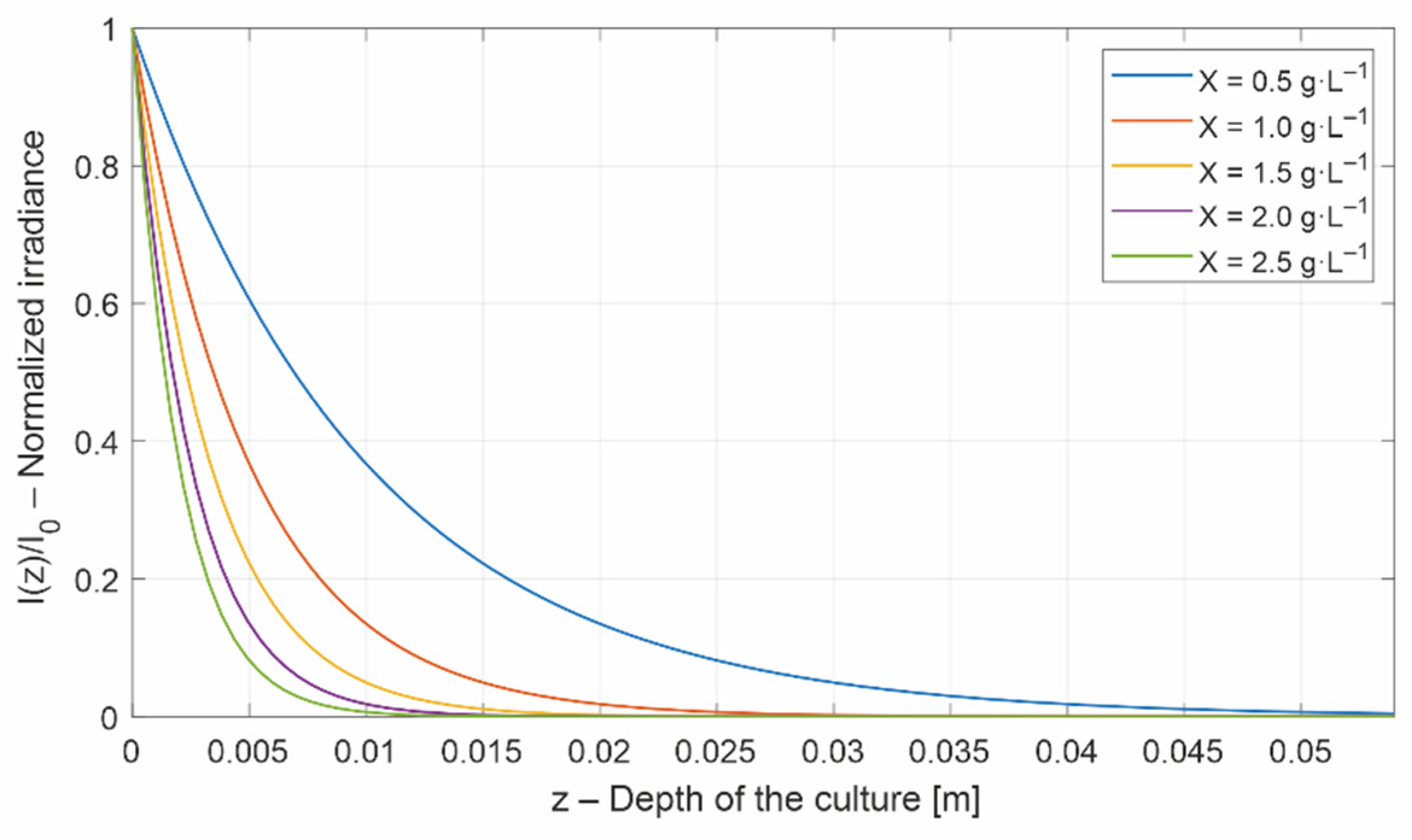
2.1. The Radiative Model

The photoautotrophic microalgae rely on light as a source of energy and can grow on inorganic nutrients such as dissolved carbon dioxide and salts of nitrogen, phosphorous, magnesium, etc. The mathematical modeling of their growth is, thus, closely related to the availability of light inside the culture.

The light required for photosynthesis has a spectral region that corresponds to the visible light (400 to 700 nm), and it is named Photosynthetically Active Radiation (PAR). Photons with other wavelengths either have not enough or they have too much energy to undertake photosynthesis and can damage the cell. Since the photons are the ones that interact with the cell photosystems, the incident PAR, $I_0$, is measured in μmole photons·m⁻²·s⁻¹ (to simplify μmol·m⁻²·s⁻¹) and hereafter named incident light intensity. The incident light intensity that touches the culture of microalgae at $z=0$ attenuates inside the PBR due to absorption phenomena and it is named irradiance and is denoted by $I$. $z$ is the depth of the culture, $z\in \left[0,L\right]$ and $L$ is the depth of the PBR. The propagation of the light inside the PBR depends on a series of factors such as medium properties, reactor geometry, the shape of cells, the concentration of pigments [21], etc. The attenuation of light inside of a microalgae culture (i.e., the irradiance) is generally described by the Lambert-Beer law, which relates the irradiance to the depth of the culture, $z$, and the properties of the liquid environment:

$$I\left(z\right)=I_0·e^{-\epsilon ·z}$$

(1)

where the constant $\epsilon$ is an extinction coefficient specific to the aquatic environment. The measuring unit of $\epsilon$ is m⁻¹ so that the exponential factor is dimensionless.

The mathematical modeling of the irradiance has been approached by various authors [21,29] aiming to describe more accurately the behavior of light in very dense media, such as microalgae cultures, where it is absorbed by the pigments but also scattered by the cells. In addition, the geometry of the PBR and the design of the lighting source are heavily influencing the attenuation of the light inside the microalgae cultures. These types of models are named radiative models.

The model adopted in this study relates the attenuation of light with the concentration of biomass, $X$, as follows [29]:

$$I\left(z\right)=I_0·e^{-\epsilon ·X·z}, \mathrm{with} \epsilon =\frac{1+\alpha }{2\alpha }{E}_a$$

(2)

where $\alpha =\sqrt{E_a/\left(E_a+2b{E}_s\right)}$ is the linear scattering modulus. For the exponential to be dimensionless, the measuring unit of the coefficient $\epsilon$ must be m²·kg⁻¹ (same as $E_a$ and $E_s$ as reported in Table 1).

The extinction coefficient, $\epsilon$, is calculated by considering the mass absorption and mass scattering coefficients (i.e., $E_a$ and $E_s$) and the backward scattering fraction, $b$. Figure 1 shows the attenuation of the light with the depth of the culture for various concentrations of biomass. To better illustrate the attenuation of light, the normalized irradiance, $I\left(z\right)/I_0$ has been calculated.

The radiative model, in Equation (2), has been developed for flat-plate PBRs, and lighted on one side. To illustrate the normalized irradiance, in Figure 1, a depth of 0.054 m has been considered. This corresponds to an airlift rectangular PBR, used in previous studies to obtain experimental data and to identify the mathematical models [37]. Figure 2 illustrates the airlift PBR along with its main components. The values of the parameters in the radiative model are given subsequently in Table 1.

2.2. The Kinetic Growth Model

The heterogeneous field created by the light inside the PBR results in growth rates that are decreasing along the depth of the culture. The coupling between the radiative models and the growth kinetics is an active research topic in PBR studies [23,31,32]. Because light energy is the most important factor for photosynthetic growth, it is considered a substrate. The specific growth rate related to photosynthesis, ${\mu }_p$, must thus be expressed as a function of the irradiance. However, the energy absorbed by microalgae is not all used for growth, a part of it being used for maintenance and, thus, a negative term is defined as the specific decay rate, ${\mu }_d$. The specific growth rate, $\mu$, has, therefore, two terms, one associated with growth and one to decay:

$$\mu ={\mu }_p-{\mu }_d$$

(3)

The PBR is considered a continuous stirred tank reactor (CSTR), which means that the concentration of any component is uniform throughout the reactor volume and can be expressed through ordinary differential equations. Nevertheless, the heterogenous light field brings a second derivation variable, the depth $z$ of the culture, which requires partial differential equations. To avoid a complex mathematical formulation, an averaged growth rate could be defined in two manners:

-

the averaged specific growth rate, $\mu \left(I_{avg}\right)$, can be calculated with an averaged irradiance, $I_{avg}$. An analytical expression for the average of the irradiance (Equation (2)) along the depth $z$ of the culture can be easily defined [30,38];

-

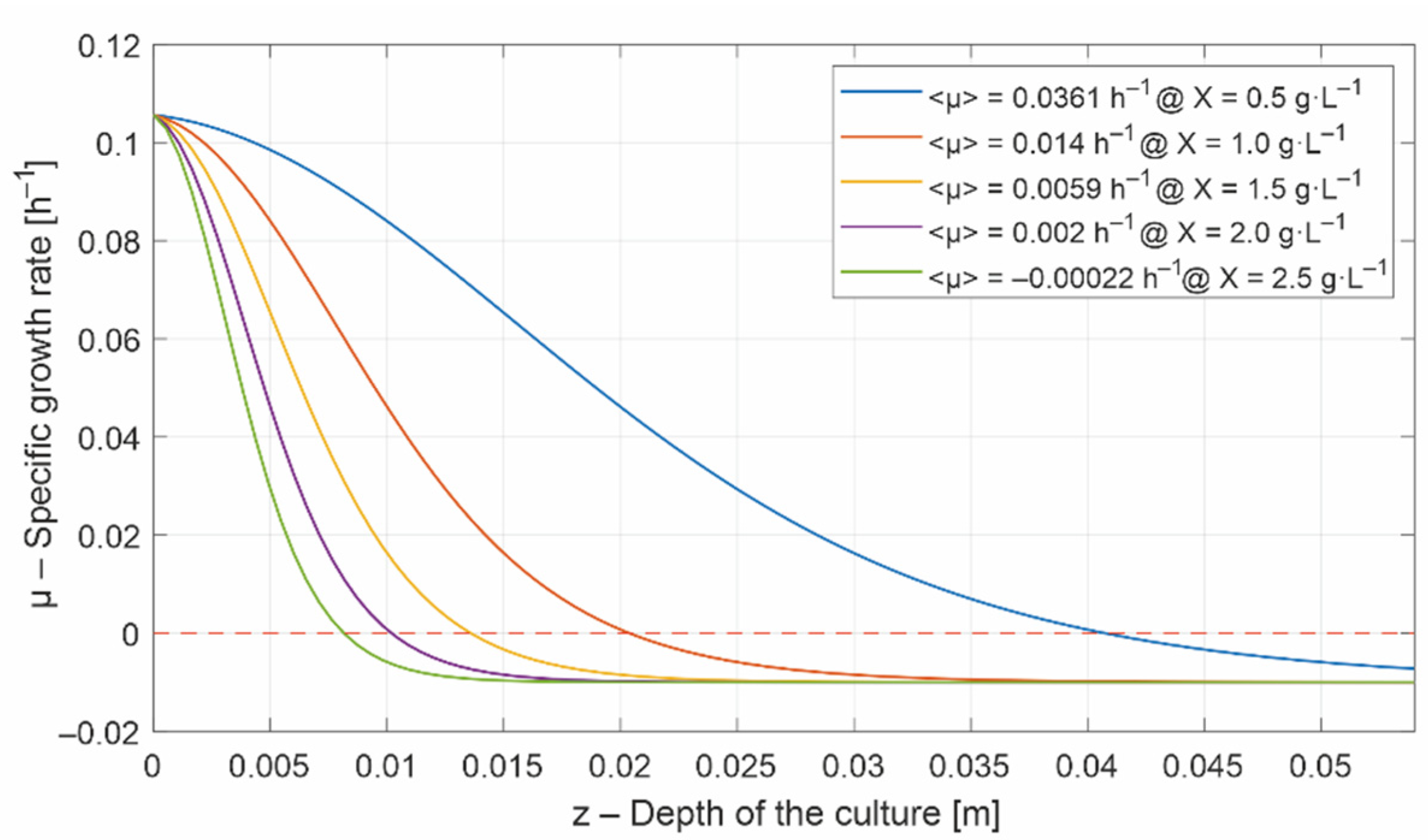
local photosynthetic responses, $\mu \left(I\left(z\right)\right)$, can be calculated for any depth $z$ of the culture. These local photosynthetic responses are simply averaged into an average photosynthetic response, $\langle \mu \rangle$ (or average specific growth rate) [31]. The $\langle \rangle$ denote an averaged value.

The present study is based on the second approach, an averaged photosynthetic response being calculated from 100 local photosynthetic responses. The specific growth rate related to photosynthesis is expressed through a classical inhibition model:

$$\langle {\mu }_p\rangle ={\mu }_o\frac{1}{L}\underset{0}{\overset{L}{{\displaystyle \int }}}\frac{I\left(z\right)}{K_S+I\left(z\right)+\frac{I{\left(z\right)}^2}{K_I}}dz$$

(4)

where ${\mu }_o$ is a kinetic parameter related to the maximum specific growth rate, $K_S$ is the saturation constant and $K_I$ is the inhibition constant. $L$ is the depth of the PBR ($z\in \left[0 L\right]$).

The specific decay rate, ${\mu }_d$, is considerably smaller than ${\mu }_o$ and, even though it varies with illumination conditions, it is considered constant here.

Figure 3 shows the specific growth rate decrease along the depth $z$ of the culture for a series of biomass concentrations. The averaged specific growth rates have also been displayed in the legend. When the culture is dense (e.g., 2.0 g·L⁻¹), the light penetrates less than a quarter of the culture, leaving the rest of it in dark. In the dark zone of the culture the specific growth rate is negative, ${\mu }_p<{\mu }_d$. The average specific growth rate is very low (i.e., 0.002 h⁻¹) for this concentration of biomass, and an incident light intensity lower than 500 μmol·m⁻²·s⁻¹ leads to the decrease of the biomass concentration. The average of the specific growth rates is justifiable because, in a CSTR, a cell is migrating continuously between the light and the dark zones.

To express the biomass as concentration, the volumetric growth rate, $r_x$, is defined:

$$\langle r_x\rangle =\langle \mu \rangle X=\langle {\mu }_p\rangle X-{\mu }_{d}X$$

(5)

2.3. The Mass Balance Model

Integrating the volumetric growth rate, the concentration of biomass, $X$, in g·L⁻¹ can be obtained:

$$\frac{dX}{dt}=\langle r_x\rangle$$

(6)

The differential equation for biomass, Equation (6), is given for a discontinuous process (batch). A batch process cannot be controlled because the reactor is filled with culture medium at the beginning, and the process takes place for a specific amount of time without any intervention. The artificially lighted PBRs, in contrast with the solar PBRs, have the incident light intensity, $I_0$, as input variable and can be controlled to obtain optimal results. These reactors are used in laboratories for data acquisition, modeling, developing and validating control strategies, production of metabolites, etc. In most cases, a batch process in an artificially lighted PBR takes place at a constant incident light intensity, but many light growth panels are now dimmable and can be controlled to obtain optimal productivities or optimal consumption of light energy.

The specific growth rate can be a function of other variables besides the light, such as substrates, pH, temperature, etc., and more equations can be added to the model. However, in this study, we consider that the substrates are in concentrations that are not limiting or inhibiting the growth and the other key factors are controlled. The biomass equation can, thus, be decoupled from other equations of substrates, for example, and be manipulated individually.

By using the incident light intensity as the control variable, the PBRs can be operated in lumostatic mode, which is controlling the $I_0$ for maintaining constant certain variables such as light-to-microalgae ratio [32,34], etc. The batch cultures with controlled incident light intensities are termed lumostatic batches. The efficiency of a lumostatic batch can be evaluated through the biomass yield on light energy, $Y$, a performance index that has the following expression [32]:

$$Y=\frac{\langle \mu \rangle \left(X-X_0\right)V}{Q}$$

(7)

where $X_0$ is the concentration of biomass, in g·L⁻¹, at the beginning of the batch ($t=0$), and $V$ is the working volume of the PBR.

The total light consumed in the batch process, $Q$, is calculated by integrating the incident light intensity over the batch time $\left[t_0 t_f\right]$:

$$Q=A\underset{t_0}{\overset{t_f}{{\displaystyle \int }}}{I}_0\left(t\right)dt=A·q$$

(8)

where $A$ is the lighted surface of the PBR. Here, $I_0\left(t\right)$ is the incident light intensity that is variable over the control horizon, while $I_0$ is used for a constant incident light intensity. $Y$ has, thus, the meaning of grams of biomass produced per moles of photons consumed (a conversion constant equal to 3600 × 10⁻⁶ is needed to express $Q$ in moles, where 3600 converts seconds to hours and 10⁻⁶ converts micromoles to moles, i.e., $Q=A·q·3600\times {10}^{-6}$).

The mathematical model used in this study consists of four ordinary differential equations (Equation (9)) and a series of algebraic equations (Equations (2)–(5) and (7)):

$$\dot{x}=\left[\begin{array}{c}\begin{array}{c}{\dot{x}}_1\\ {\dot{x}}_2\\ {\dot{x}}_3\end{array}\\ {\dot{x}}_4\end{array}\right]=\left[\begin{array}{c}\begin{array}{c}\dot{X}\\ {\dot{X}}_T\\ \dot{Q}\end{array}\\ \dot{Y}\end{array}\right]=\left[\begin{array}{c}\begin{array}{c}\langle r_x\rangle \\ \langle r_x\rangle ·V\\ A·q\end{array}\\ X_T/Q-Y\end{array}\right]$$

(9)

where $x_1$ is the concentration of biomass in g·L⁻¹, $x_2$ is the newly produced biomass in grams, $x_3$ is the amount of light consumed in moles of photons and $x_4$ is the biomass yield on light energy in grams per moles of photons. The fourth equation is in fact algebraic but is expressed as a differential equation. The integration of the mass balance model must be done with an integrator able to solve DAEs (differential-algebraic equations) such as ode15s or ode23t in Matlab [39].

The mathematical model for photosynthetic biomass growth has been validated on Chlamydomonas reinhardtii [23] and Scenedesmus quadricauda [37], strains that have been cultivated in rectangular laboratory PBRs lighted on one side. The parameters of the model used in this study are presented in Table 1.

Table 1. The parameters of the photosynthetic growth model [23,37].

Parameter	Value	Unit
$E_a$	200	m2·kg−1
$E_s$	870	m2·kg−1
$b$	0.0008	-
${\mu }_o$	0.17	h−1
$K_S$	135	μmol·m−2·s−1
$K_I$	2500	μmol·m−2·s−1
${\mu }_d$	0.01	h−1
$V$	5.74 × 10−3	m3
$A$	10.2 × 10−2	m2
$L$	0.054	m

Table 1. The parameters of the photosynthetic growth model [23,37].

Parameter	Value	Unit
$E_a$	200	m2·kg−1
$E_s$	870	m2·kg−1
$b$	0.0008	-
${\mu }_o$	0.17	h−1
$K_S$	135	μmol·m−2·s−1
$K_I$	2500	μmol·m−2·s−1
${\mu }_d$	0.01	h−1
$V$	5.74 × 10−3	m3
$A$	10.2 × 10−2	m2
$L$	0.054	m

3. The Optimal Control Problem

The objective of this paper is to find an optimal incident light intensity for which the consumption of light energy, for any amount of newly formed biomass, is minimal. To this end, reliable measurements for biomass must be available. There are direct (i.e., microscopic cell count) and indirect (e.g., dry mass, optical density, etc.) measurements of biomass concentration. While the direct measurement of biomass concentration requires microbiology skills, the dry mass is the most used measurement due to its simplicity, which requires filtering known volumes of the culture and weighing the filters before and after drying at 105 °C. The biggest disadvantage of this indirect measurement is the long time required for drying, in most cases only one value per day being available. The need for online biomass concentration measuring can be satisfied by hardware (e.g., turbidity sensors, submersible spectrophotometers, etc.) or software sensors. However, both offline and online measurements must be correlated with the dry mass.

The limited availability of online biomass measuring solutions is because the signals of the above-mentioned sensors are influenced by many factors, such as the geometry of the reactor, the composition of the culture medium, the shape of the cells, etc. A turbidity sensor, for example, is an optical sensor able to measure the suspended solids, but its signal is disturbed by the gas bubbles in the culture. Provided that it can be installed in a zone where its signal is not disturbed, the turbidity is linearly correlated with the dry mass [22], requiring the identification of two parameters, the slope, and the offset. Excellent correlation can be obtained during the exponential growth phase, while the lag, stationary, or death phases require a different set of parameters for the correlation. In a process, each new dry mass value can be used to adjust the correlation, resulting in better estimations of biomass concentration.

When no hardware sensor for biomass is available in the process, which is the case for most bioprocesses, a software sensor can be used [36]. The software sensors can be based on state estimation, regression analysis, artificial neural networks, statistical machine learning [40], etc. However, the process mechanism can be also used to estimate the biomass concentration. In this spirit, the mathematical model presented in the previous section can be used. Two of its parameters could be reidentified daily on the dry mass measurements to obtain a very good fitting, namely ${\mu }_0$ and $K_S$ (Equation (4)). To have an estimation, the mathematical model requires the initial conditions and the current process time.

We assume from here on that a value of the biomass concentration is available. Knowing the biomass concentration and the volume of the reactor, $V$, the newly produced biomass, $X_T$, can be easily calculated (Equation (9)). To achieve the goal of finding the optimal incident light intensity for which the biomass yield on light energy is maximal, the light source must be dimmable and controlled by the process computer. The light sources can be calibrated with light meters, correlating the input voltage with the incident light intensity in μmol·m⁻²·s⁻¹. To calculate the amount of light consumed, $Q$, the model requires the incident light intensity, $I_0$, the lighted surface of the PBR, and the current process time. By dividing the newly produced biomass by the amount of light consumed, the biomass yield on light energy can be easily calculated ($Y=X_T/Q$).

Integrating the mathematical model over a wide range of incident light intensities, 1 to 2000 μmol·m⁻²·s⁻¹, it can be found that the biomass yield on light energy, $Y$, is a unimodal unidimensional function whose maximum gives the optimal incident light intensity, $I_{0\left(opt\right)}$ (Figure 4). The optimization of $Y$ can be done with unidimensional optimization methods [41] such as the golden section search, the parabolic interpolation, etc. The constraints to which the input variable $I_0$ is subjected have been selected from a technological point of view, 1 μmol·m⁻²·s⁻¹ to avoid division by zero (Equation (7)), and 2000 μmol·m⁻²·s⁻¹ is the maximal sun radiation on a summer day.

Figure 4 displays the response of the system at various incident light intensities which have been obtained on a one-hour horizon.

The simulations have been made on a horizon of one hour, mentioning that simulations on wider horizons are similar in terms of $I_{0\left(opt\right)}$, as can be seen in Figure 5. The initial conditions used for simulations are $X\left(0\right)=1.1386$ g·L⁻¹, $X_T\left(0\right)=4.4690$ g (not displayed in Figure 4), $Q\left(0\right)=9.18$ g·mol photon⁻¹, which means that $Y\left(0\right)=X_T\left(0\right)/Q\left(0\right)=0.4868$.

The mathematical model for the photosynthetic growth of microalgae can give even more information on the process. The specific growth rate, $\mu$, provides valuable bounds for the control variable $I_0$:

-

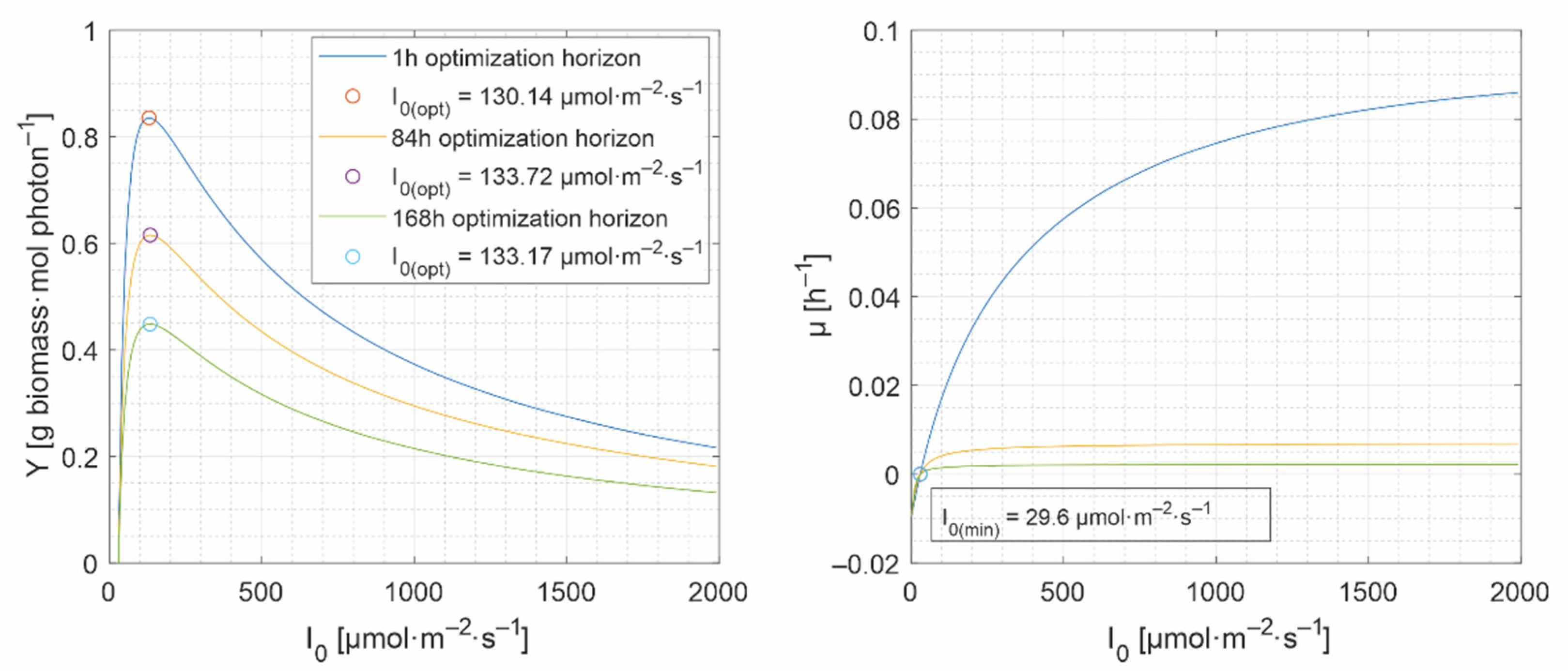
a lower bound, $I_{0\left(min\right)}$, under which the biomass would decrease. Below $I_{0\left(min\right)}$ the specific growth rate is negative (Figure 4), and

-

an upper bound, $I_{0\left(max\right)}$, which is set in Figure 4 at 80% of the maximum growth rate.

The biomass yield on light energy, $Y$, can thus be used in the optimization process. The optimal control problem starts from the photosynthetic growth model which has been presented in the second section. It consists of a system of four differential equations, therefore the state vector is:

$$x\left(t\right)={\left[\begin{array}{cccc}\dot{X}\left(t\right)& {\dot{X}}_T\left(t\right)& \dot{Q}\left(t\right)& \dot{Y}\left(t\right)\end{array}\right]}^T$$

(10)

The input variable for the system is the incident light intensity:

$$u\left(t\right)=I_0\left(t\right)$$

(11)

The optimal control problem is subjected to the following constraints:

-

the control horizon: $t_0\le t\le t_f$, where $t_0$ and $t_f$ are the initial and the final time of the control horizon (the batch period),

-

the initial conditions: $x\left(t_0\right)=x_0$,

-

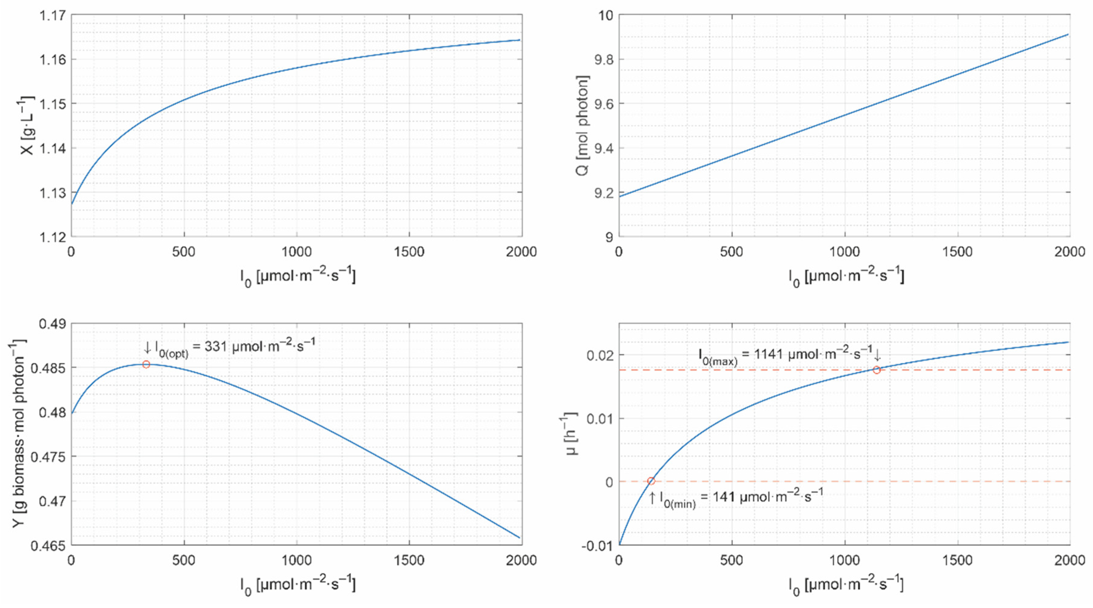
the set of lower and upper bounds: $I_{0\left(min\right)}\le I_0\left(t\right)\le I_{0\left(max\right)}$, with $t_0\le t\le t_f$. The lower bound, $I_{0\left(min\right)}$, is critical because the biomass decreases under this value, while the upper bound is not, and can remain constant (e.g., 2000 μmol·m⁻²·s⁻¹). Even though $I_{0\left(max\right)}$ can inhibit the microalgae growth, it is attenuated inside the culture. The lower and the upper bounds are required by most of the unidimensional optimization methods [41], e.g., fminbnd function in Matlab.

The general form of the optimal control problem which searches the control $u(·)$ that maximizes the objective function $J$ is:

$$J\left(x,u\right)={{\displaystyle \int }}_{t_0}^{t_f}L\left(x\left(t\right),u\left(t\right),t\right)dt$$

(12)

where the term $L\left(x,u,t\right)$ is the intermediate cost function. The optimal control aims to find the state and control trajectories $x$ and $u$ so that $J\left(x,u\right)$ is maximized:

$$x^{*}, u^{*}=\arg \underset{x,u}{\max }J\left(x,u\right) \mathrm{such} \mathrm{that} \dot{x}\left(t\right)=f\left(x\left(t\right),u\left(t\right)\right) \mathrm{for} \mathrm{all} t$$

(13)

Finding the optimal incident light intensity for which the consumption of light energy, for any amount of newly formed biomass, is minimal, requires maximizing the biomass yield on light energy, thus the optimal control input has the following form:

$$I_{0\left(opt\right)}=\underset{I_0\left(t\right), t_0\le t\le t_f}{\arg \max }Y\left(t\right)$$

(14)

The optimization and control horizons are usually different, while the optimization can be performed on the entire batch time $\left[t_0 t_f\right]$, the control horizon is usually lower, resulting that the $u\left(t\right)$ is the vector of input variables. If $t_k$ is the current time, $t_0\le t_k\le t_f$, the control horizon can be $\left[t_k t_{k+p}\right]$. Figure 5 displays the results obtained at the optimization of the photosynthetic growth process range of incident light intensities of 1 to 2000 μmol·m⁻²·s⁻¹. As has been the case previously (Figure 4), the results are the final values of the states, after the integration of the model for one hour with each $I_0\in \left[1, 2000\right]$ μmol·m⁻²·s⁻¹. Optimization on three horizons is presented, 1, 84, and 168 h, taking a seven-day cultivation process as a reference. The initial condition for biomass is $X\left(0\right)=0.3$ g·L⁻¹, while the other states have been set to zero ($Q\left(0\right)$ should be set to a very small positive value to avoid division by zero). It can be observed that the optimal incident light intensity is similar, regardless of the length of the optimization horizon. Comparing Figure 4 with 5, it can be observed that higher concentrations of biomass require higher concentrations of light to reach an optimal yield, $X\left(0\right)=0.3$ g·L⁻¹ requires ≈ 130 μmol·m⁻²·s⁻¹ while $X\left(0\right)=1.1386$ g·L⁻¹ requires ≈ 331 μmol·m⁻²·s⁻¹. This points out the need for an increase in the incident light intensity as the biomass grows. Working with constant light throughout the photosynthetic growth process could require more light energy to obtain the same amount of biomass compared to an increasing light profile. This problem has been addressed in [32] by controlling the light-to-microalgae ratio, but the present paper takes it a step further by investigating the optimization of a lumostatic batch (i.e., a batch with variable incident light intensity).

The disadvantage of using the biomass yield on light energy, $Y$, as objective function is that it lacks a scaling factor to push the concentration of biomass higher. $Y$ assures that the consumption of light energy is optimal, but this could result in low concentrations of biomass. In this regard, the information of the specific growth rate, $\mu$, which is already used to determine the lower bound $I_{0\left(min\right)}$, can be used as follows:

$$I_{0\left(opt\right)}=\underset{I_0\left(t\right), t_0\le t\le t_f}{\arg \max }\left(Y\left(t\right)+w*\mu \left(t\right)\right)$$

(15)

where $w$ is a positive scaling factor. $\mu \left(t\right)$ has the effect of shifting the optimum to the right and, along with the scaling factor, any increasing $I_0\left(t\right)$ profile can be obtained. Thus, higher concentrations of biomass can be obtained, while the consumed amount of light energy is minimal.

The desired increasing light profile can be obtained by iteratively optimizing the process for any given current time and state. In this regard, a closed-loop control system has been proposed in the following section.

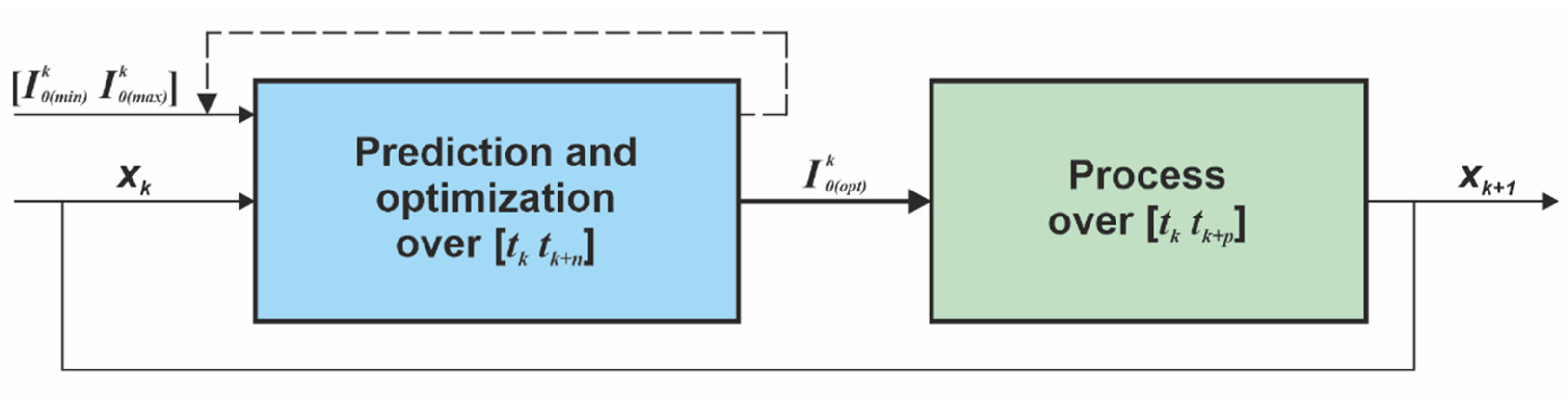
4. The Closed-Loop Control System

4.1. The Control Structure

The objective of this work is to provide a closed-loop solution for the optimal control problem presented in the previous section; in other words, an optimal controller that provides an incident light intensity value to the process, for each sampling period. Figure 6 presents the closed-loop control structure proposed in this work. The optimal controller calculates the optimal incident light intensity, $I_{0\left(opt\right)}$, over the optimization horizon $\left[t_k t_{k+n}\right]$, with $k=0,\dots ,f$ where $t_0$ and $t_f$ are the beginning and the end of the photosynthetic growth process. $n$ is a positive constant, expressed in hours, which is the length of the optimization horizon. To calculate the current control variable, $I_{0\left(opt\right)}^k$, the optimal controller requires the current state of the process, $x_k$, and current time, $t_k$. Thus, the optimal controller must predict the future evolution of the process, and calculate the optimal incident light intensity based on these predictions. This requires a process model to be included in the optimal controller. The lower bound, $I_{0\left(min\right)}$, can be found through a simple numerical root finding method (e.g., the bisection method) because $\mu$ intersects the Ox axis only once. There is no specific method to find the upper bound, $I_{0\left(max\right)}$, in Figure 4 being set at 80% of the specific growth rate obtained for 2000 μmol·m⁻²·s⁻¹. The current lower and upper bounds, $I_{0\left(min\right)}^k\le I_{0\left(opt\right)}^k\le I_{0\left(max\right)}^k$, are calculated with the process model before the optimization procedure.

The sampling period of the photosynthetic growth process is $\left[t_k t_{k+p}\right]$, where $p$ is a positive constant, expressed in hours, which is the length of the sampling period (usually $n\ge p$). The process generates a new set of values for the state variables, $x_{k+1}$, which are used by the optimal controller to calculate a new input, along with the current time and current bounds.

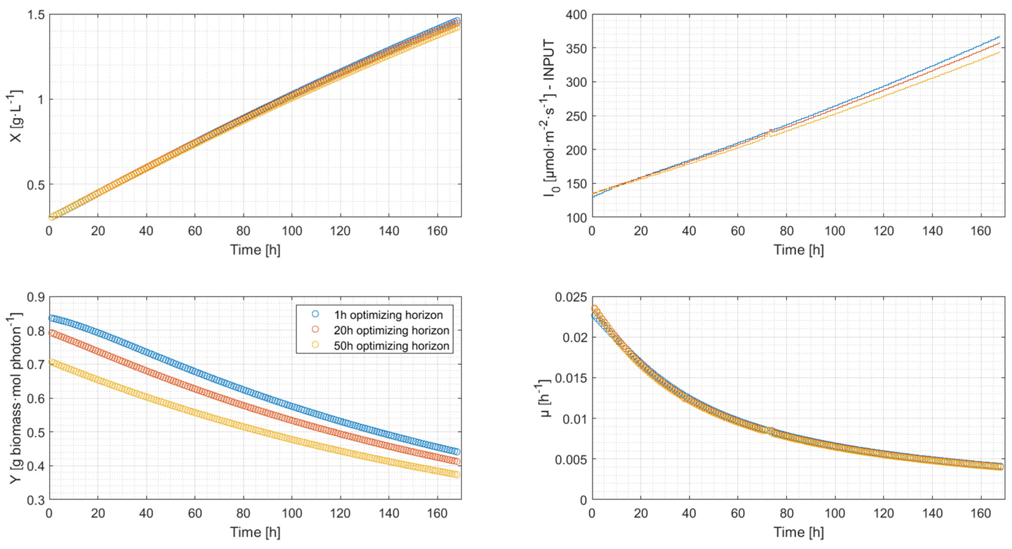
4.2. Simulation Results

A seven-day (168 h) photosynthetic batch process has been used as reference to validate the optimal controller in simulation. The initial conditions used for all simulations in this section are $X\left(0\right)=0.3$ g·L⁻¹, while the other three states have been set to zero (same as for Figure 5).

Figure 7 displays the results obtained with the closed loop optimal controller on a 1-h sampling period, $p=1$, $\left[t_k t_{k+1}\right]$. The behavior observed in Figure 5 is also observed in closed loop, and the length of the optimization horizon is not significantly influencing the process. As the optimization horizon is bigger, slightly lower biomass values are obtained. For example, the 20-h optimization horizon results in a biomass concentration of only 0.96% lower in comparison with the 1-h optimization horizon. Also, lower $Y$ values give similar $I_{0\left(opt\right)}$, because $Y$ decreases throughout the batch culture.

A higher optimization horizon increases computational complexity of the algorithm and thus a 1-h horizon is recommended.

In addition to the optimization horizon, the sampling period must be determined. Given that the biological process is slow, a 1-h period has been considered. This period can be shortened by the capacity of the process computer to measure the states and calculate a new control variable. Nevertheless, longer sampling periods have been investigated for cases where an online biomass sensor is not available, and the optimization procedure cannot be performed online. This would require the daily reidentification of the mathematical model based on dry mass measurements and the optimization of the process based on the model predictions, the operator being able to insert a new command every 12 h.

Figure 8 shows the evolution of the process with the closed loop optimal controller on 1-h and 12-h sampling periods. Similar results are obtained in terms of biomass growth, which proves that longer sampling periods are feasible for systems that have certain limitations.

The results presented in Figure 7 and Figure 8 are obtained using the biomass yield on light energy as objective function. Regardless of the optimization horizon and the sampling period, the concentration of biomass is slightly lower than $1.5$ g·L⁻¹. Further increasing the sampling period results in significantly lower concentrations of biomass, as can be seen in

Table 2. Influence of the sampling period on the concentration of biomass.

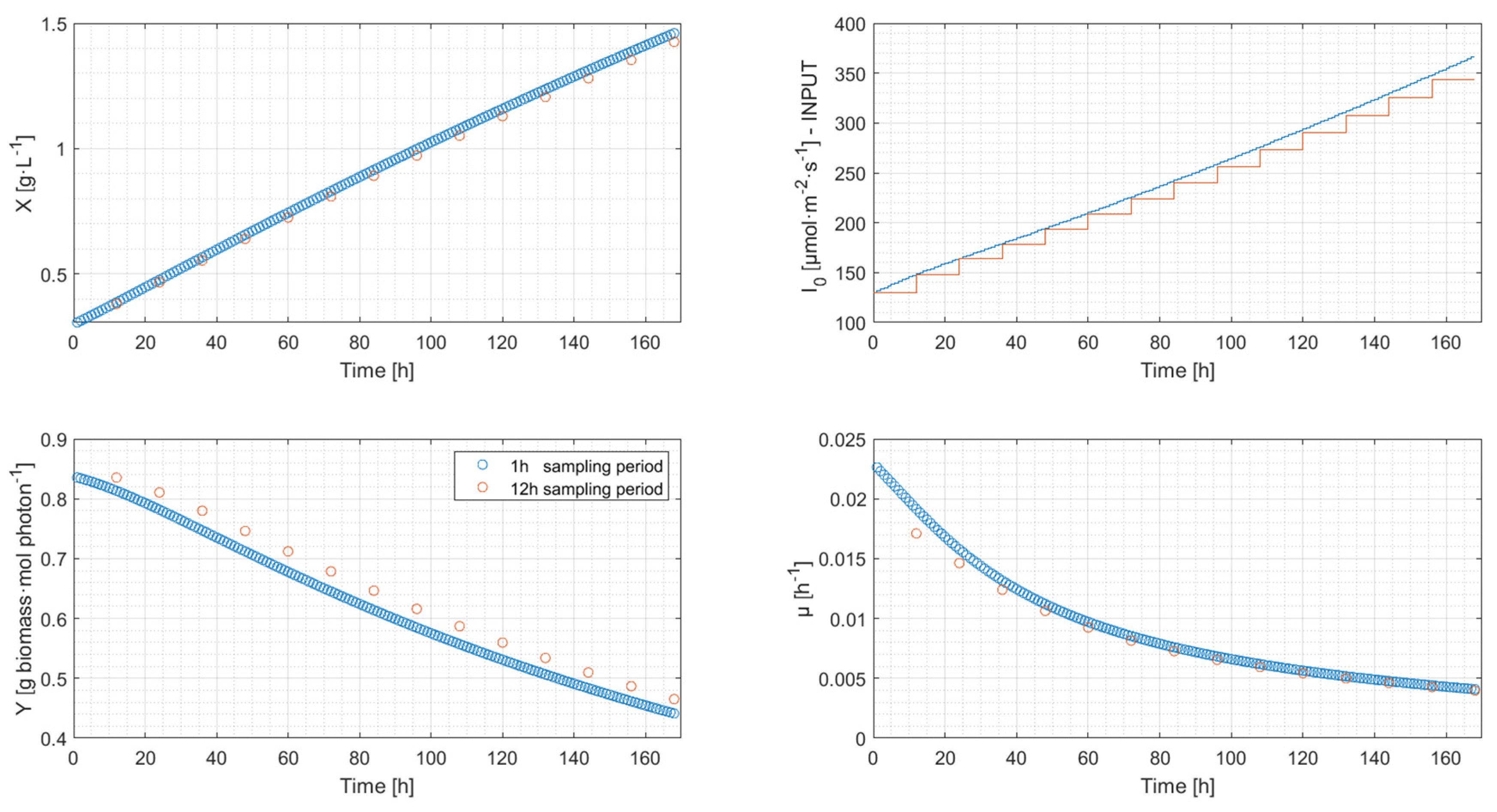
Length of the Sampling Period	Biomass Concentration [g·L−1]	Decrease [%]
1-h	1.460
12-h	1.418	−2.88
24-h	1.374	−5.89
168-h	0.942	−35.48

. A constant incident light intensity of 133.17 μmol·m⁻²·s⁻¹ throughout the entire batch (see also Figure 5) results in a biomass concentration 35.48% lower compared with the 1-h sampling period.

Higher biomass concentrations can be obtained with higher incident light intensities, and this can be achieved by using the objective function in Equation (15).

Figure 9 shows the simulation results on a seven-day batch for different weighing factors. A higher $w$ results in a higher concentration of biomass, providing that the amount of light energy consumed is minimal. Because the second term of the objective function $w*\mu \left(t\right)$, is considerably smaller than $Y\left(t\right)$, both objective functions have generated similar results (3rd and 4th graphs of Figure 9). The scaling factor thus provides the means to adapt the optimization algorithm to the technological limitations of the systems (i.e., the maximal output of the light source) and allows for the obtaining of a desired amount of biomass.

5. Conclusions

The paper proposes a closed-loop control system for the process of photosynthetic growth of microalgae. A simple mathematical model with four state variables has been proposed for predicting the evolution of biomass concentration, the total quantity of newly formed biomass, the total amount of consumed light, and the biomass yield on light energy. It has been found that the biomass yield on light energy, $Y$, is a unimodal function on the admissible range of incident light intensities, $I_0$, which can be used to optimize the lumostatic batch culture. Maximizing $Y$ results in finding the optimal incident light intensity for which the consumption of light energy, for any amount of newly formed biomass, is minimal. A second objective function has been proposed by adding a second term to $Y$, which consists of using the specific growth rate along with a weighing factor. This new term shifts the optimum to the right and allows for the obtaining of higher concentrations of biomass. While the first objective function ensures an optimal consumption of light energy, the second objective function also targets a higher amount of newly formed biomass. The developed optimization algorithms have been integrated into a closed-loop structure. The optimal controller is generating an increasing light profile which is more efficient, in terms of consumed energy, compared with a constant light batch. It has been proven that a 1-h optimization horizon is sufficient for obtaining good results and reducing the complexity of the computation. The sampling period has also been investigated, providing a solution for the processes with certain limitations. Finally, it has been shown that tuning the weighing factor has led to the achievement of the desired increasing light profile. The results have been validated in simulation; a reliable solution has been proposed for the optimal control of lumostatic batches.

References

- Singh, J.; Chandra Saxena, R. An Introduction to Microalgae: Diversity and Significance. In Handbook of Marine Microalgae; Kim, S.-K., Ed.; Academic Press: Cambridge, MA, USA, 2015; pp. 11–24. [Google Scholar] [CrossRef]
- Pagels, F.; Salvaterra, D.; Amaro, H.M.; Guedes, A.C. Pigments from microalgae. In Handbook of Microalgae-Based Processes and Products; Jacob-Lopes, E., Maroneze, M.M., Queiroz, M.I., Zepka, L.Q., Eds.; Academic Press: Cambridge, MA, USA, 2020; pp. 465–492. [Google Scholar] [CrossRef]
- Amorim, M.L.; Soares, J.; Coimbra, J.S.R.; Leite, M.O.; Albino, L.F.T.; Martins, M.A. Microalgae proteins: Production, separation, isolation, quantification, and application in food and feed. Crit. Rev. Food Sci. Nutr. 2021, 61, 1976–2002. [Google Scholar] [CrossRef] [PubMed]
- Mahata, C.; Das, P.; Khan, S.; Thaher, M.I.A.; Abdul Quadir, M.; Annamalai, S.N.; Al Jabri, H. The Potential of Marine Microalgae for the Production of Food, Feed, and Fuel (3F). Fermentation 2022, 8, 316. [Google Scholar] [CrossRef]
- Borowiak, D.; Krzywonos, M. Bioenergy, Biofuels, Lipids and Pigments—Research Trends in the Use of Microalgae Grown in Photobioreactors. Energies 2022, 15, 5357. [Google Scholar] [CrossRef]
- Lupette, J.; Benning, C. Human health benefits of very-long-chain polyunsaturated fatty acids from microalgae. Biochimie 2020, 178, 15–25. [Google Scholar] [CrossRef] [PubMed]
- Santin, A.; Balzano, S.; Russo, M.T.; Palma Esposito, F.; Ferrante, M.I.; Blasio, M.; Cavalletti, E.; Sardo, A. Microalgae-Based PUFAs for Food and Feed: Current Applications, Future Possibilities, and Constraints. J. Mar. Sci. Eng. 2022, 10, 844. [Google Scholar] [CrossRef]
- Jansen, M.; Wijffels, R.H.; Barbosa, M.J. Microalgae based production of single-cell protein. Curr. Opin. Biotechnol. 2022, 75, 102705. [Google Scholar] [CrossRef]
- Lucakova, S.; Branyikova, I.; Hayes, M. Microalgal Proteins and Bioactives for Food, Feed, and Other Applications. Appl. Sci. 2022, 12, 4402. [Google Scholar] [CrossRef]
- Alishah Aratboni, H.; Rafiei, N.; Garcia-Granados, R.; Alemzadeh, A.; Morones-Ramírez, J.R. Biomass and lipid induction strategies in microalgae for biofuel production and other applications. Microb. Cell. Fact. 2019, 18, 178. [Google Scholar] [CrossRef] [PubMed] [Green Version]
- Krishnamoorthy, A.; Rodriguez, C.; Durrant, A. Sustainable Approaches to Microalgal Pre-Treatment Techniques for Biodiesel Production: A Review. Sustainability 2022, 14, 9953. [Google Scholar] [CrossRef]
- Cheng, D.; Li, D.; Yuan, Y.; Zhou, L.; Li, X.; Wu, T.; Wang, L.; Zhao, Q.; Wei, W.; Sun, Y. Improving carbohydrate and starch accumulation in Chlorella sp. AE10 by a novel two-stage process with cell dilution. Biotechnol. Biofuels 2017, 10, 75. [Google Scholar] [CrossRef] [PubMed]
- Olguín, E.J.; Sánchez-Galván, G.; Arias-Olguín, I.I.; Melo, F.J.; González-Portela, R.E.; Cruz, L.; De Philippis, R.; Adessi, A. Microalgae-Based Biorefineries: Challenges and Future Trends to Produce Carbohydrate Enriched Biomass, High-Added Value Products and Bioactive Compounds. Biology 2022, 11, 1146. [Google Scholar] [CrossRef] [PubMed]
- Al-Jabri, H.; Das, P.; Khan, S.; Thaher, M.; AbdulQuadir, M. Treatment of Wastewaters by Microalgae and the Potential Applications of the Produced Biomass—A Review. Water 2021, 13, 27. [Google Scholar] [CrossRef]
- Ruiz, J.; Olivieri, G.; de Vree, J.; Bosma, R.; Willems, P.; Reith, J.H.; Eppink, M.H.M.; Kleinegris, D.M.M.; Wijffels, R.H.; Barbosa, M.J. Towards industrial products from microalgae. Energy Environ. Sci. 2016, 10, 3036–3043. [Google Scholar] [CrossRef]
- Severo, I.A.; Siqueira, S.F.; Deprá, M.C.; Maroneze, M.M.; Zepka, L.Q.; Jacob-Lopes, E. Biodiesel facilities: What can we address to make biorefineries commercially competitive? Renew. Sustain. Energy Rev. 2019, 112, 686–705. [Google Scholar] [CrossRef]
- Ahmad, A.; Banat, F.; Alsafar, H.; Hasan, S.W. Algae biotechnology for industrial wastewater treatment, bioenergy production, and high-value bioproducts. Sci. Total Environ. 2022, 806, 150585. [Google Scholar] [CrossRef] [PubMed]
- Molazadeh, M.; Ahmadzadeh, H.; Pourianfar, H.R.; Lyon, S.; Rampelotto, P.H. The Use of Microalgae for Coupling Wastewater Treatment with CO2 Biofixation. Front. Bioeng. Biotechnol. 2019, 7, 42. [Google Scholar] [CrossRef] [PubMed]
- Acién Fernández, F.G.; Fernández Sevilla, J.M.; Molina Grima, E. Photobioreactors for the production of microalgae. Rev. Environ. Sci. Biotechnol. 2013, 12, 131–151. [Google Scholar] [CrossRef]
- Legrand, J.; Arnaud, A.; Pruvost, J. A review on photobioreactor design and modelling for microalgae production. React. Chem. Eng. 2021, 6, 1134–1151. [Google Scholar] [CrossRef]
- Pottier, L.; Pruvost, J.; Deremetz, J.; Cornet, J.F.; Legrand, J.; Dussap, C.G. A fully predictive model for one-dimensional light attenuation by Chlamydomonas reinhardtii in a torus photobioreactor. Biotechnol. Bioeng. 2005, 91, 569–582. [Google Scholar] [CrossRef] [PubMed]
- Ifrim, G.A.; Titica, M.; Barbu, M.; Boillereaux, L.; Cogne, G.; Caraman, S.; Legrand, J. Multivariable Feedback Linearizing Control of Chlamydomonas reinhardtii Photoautotrophic Growth Process in a Torus Photobioreactor. Chem. Eng. J. 2013, 218, 191–203. [Google Scholar] [CrossRef]
- Ifrim, G.A.; Titica, M.; Cogne, G.; Boillereaux, L.; Legrand, J.; Caraman, S. Dynamic pH Model for Autotrophic Growth of Microalgae in Photobioreactor: A Tool for Monitoring and Control Purposes. AIChe J. 2014, 60, 585–599. [Google Scholar] [CrossRef]
- Grognard, F.; Akhmetzhanov, A.R.; Masci, P.; Bernard, O. Optimization of a photobioreactor biomass production using natural light. In Proceedings of the 49th IEEE Conference on Decision and Control (CDC), Atlanta, GA, USA, 15–17 December 2010; pp. 4691–4696. [Google Scholar] [CrossRef]
- Grognard, F.; Akhmetzhanov, A.R.; Bernard, O. Optimal strategies for biomass productivity maximization in a photobioreactor using natural light. Automatica 2014, 50, 359–368. [Google Scholar] [CrossRef]
- de Andrade, G.A.; Berenguel, M.; Guzmán, J.L.; Pagano, D.J.; Acién, F.G. Optimization of biomass production in outdoor tubular photobioreactors. J. Process Control. 2016, 37, 58–69. [Google Scholar] [CrossRef]
- Yoo, S.J.; Jeong, D.H.; Kim, J.H.; Lee, J.M. Optimization of microalgal photobioreactor system using model predictive control with experimental validation. Bioprocess Biosyst. Eng. 2016, 39, 1235–1246. [Google Scholar] [CrossRef] [PubMed]
- Carreño-Zagarra, J.J.; Guzmán, J.L.; Moreno, J.C.; Villamizar, R. Linear active disturbance rejection control for a raceway photobioreactor. Control. Eng. Pract. 2019, 85, 271–279. [Google Scholar] [CrossRef]
- Cornet, J.P.; Dussap, C.G. A Simple and Reliable Formula for Assessment of Maximum Volumetric Productivities in Photobioreactors. Biotechnol. Prog. 2009, 25, 424–435. [Google Scholar] [CrossRef] [PubMed]
- Jayaraman, S.K.; Rhinehart, R.R. Modeling and Optimization of Algae Growth. Ind. Eng. Chem. Res. 2015, 54, 8063–8071. [Google Scholar] [CrossRef]
- Degrenne, B.; Pruvost, J.; Titica, M.; Takache, H.; Legrand, J. Kinetic modeling of light limitation and sulfur deprivation effects in the induction of hydrogen production with Chlamydomonas reinhardtii. Part II: Definition of model-based protocols and experimental validation. Biotechnol. Bioeng. 2011, 108, 2288–2299. [Google Scholar] [CrossRef] [PubMed]
- Ifrim, G.A.; Titica, M.; Boillereaux, L.; Caraman, S. Feedback linearizing control of light-to-microalgae ratio in artificially lighted photobioreactors. In Proceedings of the 12th IFAC Symposium on Computer Applications in Biotechnology (CAB), Mumbai, India, 16–18 December 2013; pp. 60–65. [Google Scholar] [CrossRef]
- Eriksen, N.T.; Geest, T.; Iversen, J.J.L. Phototrophic growth in the lumostat: A photo-bioreactor with on-line optimization of light intensity. J. Appl. Phycol. 1996, 8, 345–352. [Google Scholar] [CrossRef]
- Tebbani, S.; Titica, M.; Ifrim, G.; Barbu, M.; Caraman, S. Optimal Operation of a Lumostatic Microalgae Cultivation Process. In Developments in Model-Based Optimization and Control: Distributed Control and Industrial Applications; Olaru, S., Grancharova, A., Lobo Pereira, F., Eds.; Springer International Publishing: Berlin/Heidelberg, Germany, 2015; pp. 209–235. [Google Scholar] [CrossRef]
- Kandilian, R.; Tsao, T.C.; Pilon, L. Control of incident irradiance on a batch operated flat-plate photobioreactor. Chem. Eng. Sci. 2014, 119, 99–108. [Google Scholar] [CrossRef]
- Minzu, V.; Ifrim, G.; Arama, I. Control of Microalgae Growth in Artificially Lighted Photobioreactors Using Metaheuristic-Based Predictions. Sensors 2021, 21, 8065. [Google Scholar] [CrossRef] [PubMed]
- Ifrim, G.A.; Titica, M.; Deppe, S.; Frahm, B.; Barbu, M.; Caraman, S. Multivariable control strategy for the photosynthetic cultures of microalgae. In Proceedings of the 23rd International Conference on System Theory, Control and Computing (ICSTCC), Sinaia, Romania, 9–11 October 2019; pp. 218–223. [Google Scholar] [CrossRef]
- Gassenmeier, V.; Deppe, S.; Hernández Rodríguez, T.; Kuhfuß, F.; Moser, A.; Hass, V.C.; Kuchemüller, K.B.; Pörtner, R.; Möller, J.; Ifrim, G.; et al. Model-assisted DoE applied to microalgae processes. Curr. Res. Biotechnol. 2022, 4, 102–118. [Google Scholar] [CrossRef]
- Shampine, L.F.; Reichelt, M.W.; Kierzenka, J.A. Solving Index-1 DAEs in MATLAB and Simulink. SIAM Rev. 1999, 41, 538–552. [Google Scholar] [CrossRef]
- Yan, P.; Gai, M.; Wang, Y.; Gao, X. Review of Soft Sensors in Anaerobic Digestion Process. Processes 2021, 9, 1434. [Google Scholar] [CrossRef]
- Antoniu, A.; Lu, W.S. Practical Optimization. In Algorithms and Engineering Applications; Springer: New York, NY, USA, 2007. [Google Scholar] [CrossRef] [Green Version]