


Hyperspectral Band Selection via Band Grouping and Adaptive Multi-Graph Constraint
Abstract
1. Introduction
1.1. Overview and Motivation
1.2. Contributions
- 1.
- The method of band grouping is used originally to process hyperspectral data, which mines the context information of the whole spectral dimension and avoids redundancy in order to obtain the more accurate selected subset.
- 2.
- An unsupervised adaptive graph constraint is introduced into the hyperspectral band selection model. The global similarity matrix is reconstructed by the linear combination of the similarity matrix of all groups with adaptive weighting.
- 3.
- An iterative optimization algorithm is proposed for obtaining the optimal weights of the proposed model. Moreover, the objective function is solved by the algorithm to select the optimal subset of bands. Through several experiments, the results are compared with the results of previous methods to verify the efficiency of our algorithm.
1.3. Organization
2. Related Works
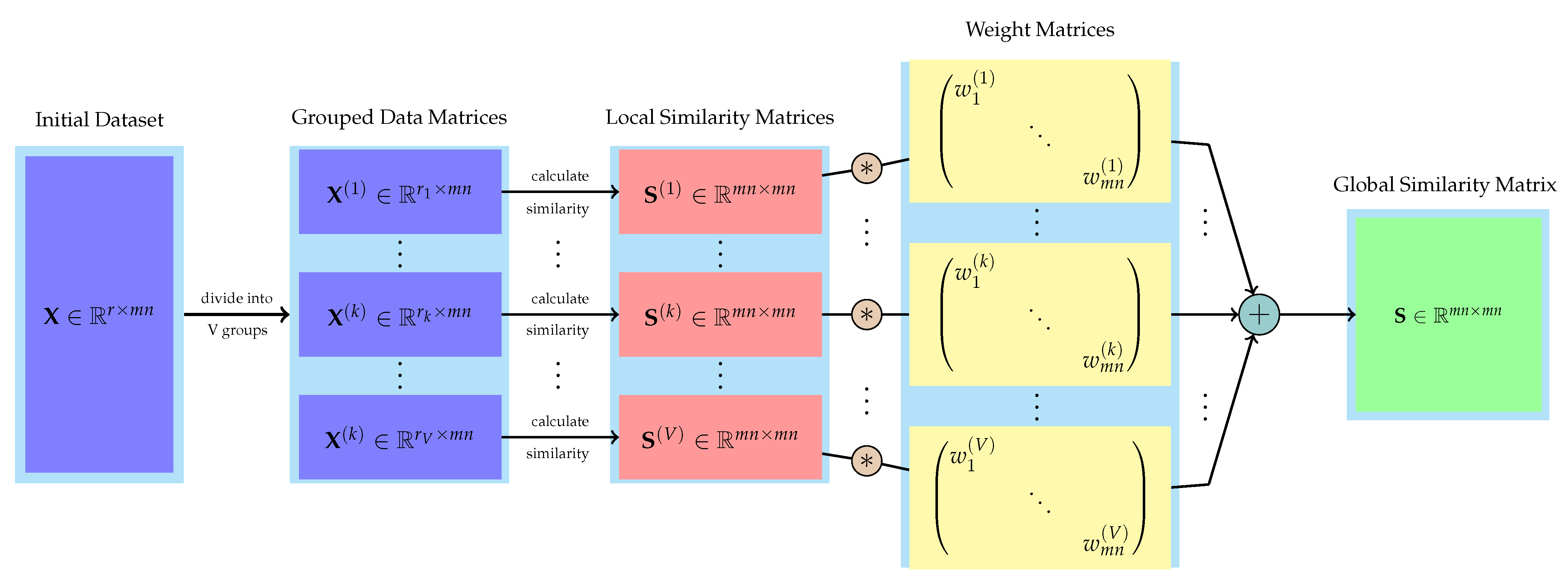
3. Methods
3.1. Model Construction
- 1.
- , i.e., is a real symmetric matrix;
- 2.
- For any sample and , the similarity value should between 0 and 1, i.e., . It means that the closer the similarity is to 1, the more similar the two columns of data;
- 3.
- The sum of each row (or each column) of equals to 1, i.e., and .
3.2. Model Optimization
3.2.1. Fix , , and : Update
3.2.2. Fix , , and : Update
3.2.3. Fix , , and : Update
3.2.4. Fix , , and : Update
| Algorithm 1: Alternative iterative algorithm to solve Equation (8). |
Input: The data matrix , , and the hyperparameters . Output:K selected bands.  |
4. Experiments
4.1. Dataset Descriptions
4.1.1. ROSIS Pavia University Image
4.1.2. AVIRIS Indian Pines Image
4.1.3. AVIRIS Salinas Scene
4.1.4. Botswana Image
4.1.5. University of Houston
4.2. Methods Taken for Comparison
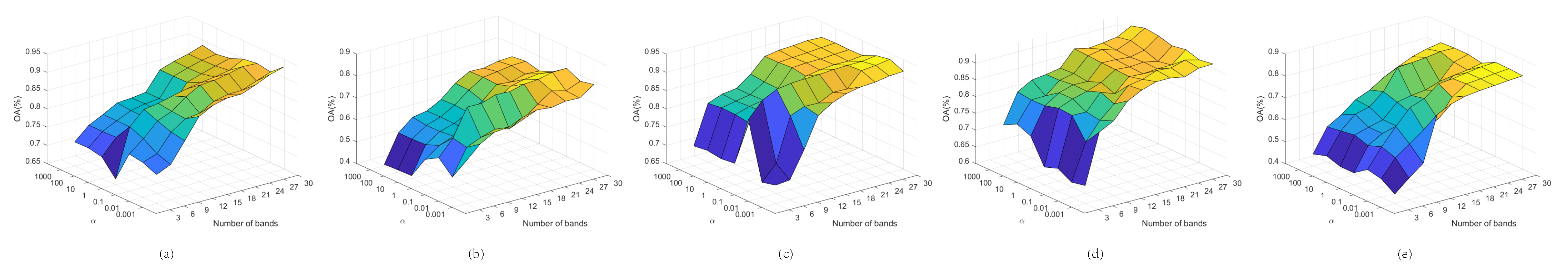
4.3. Experimental Setting
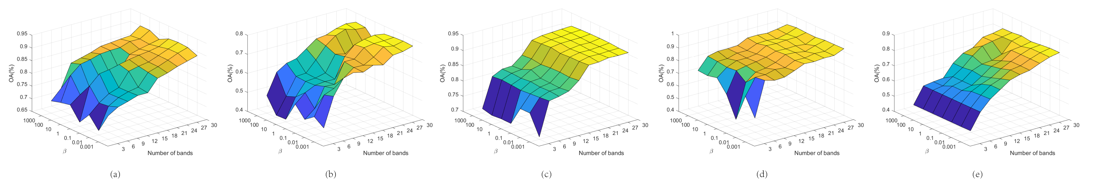
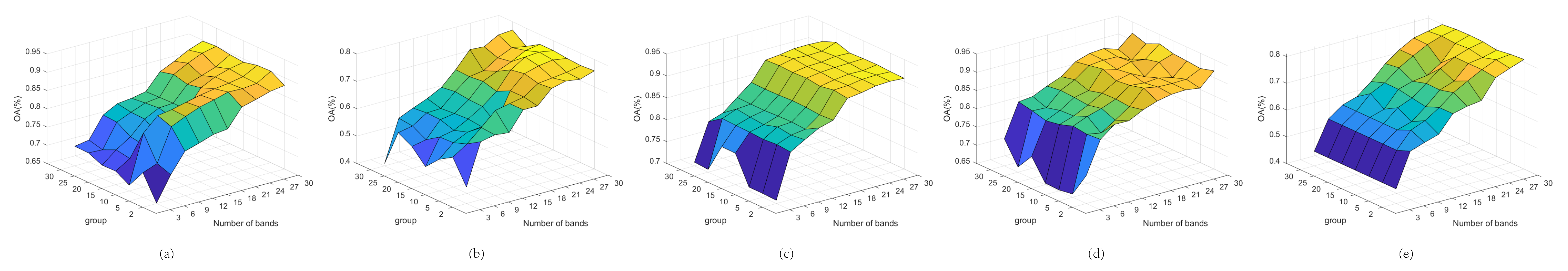
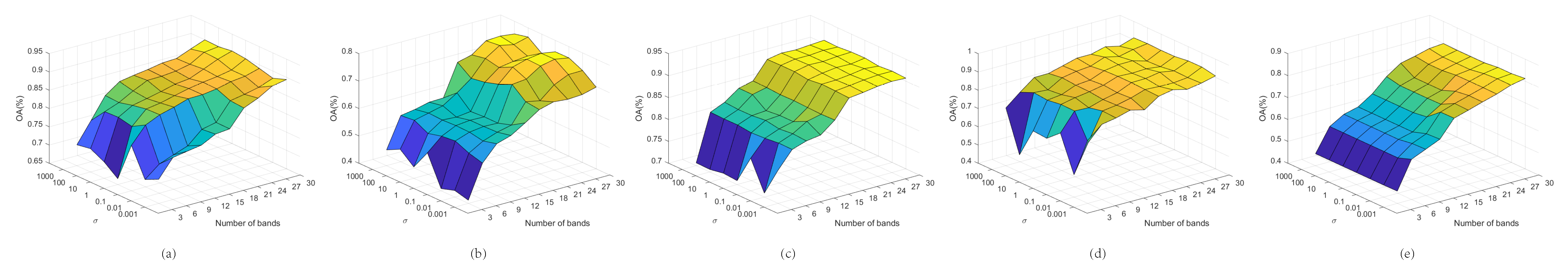
4.4. Result Analysis
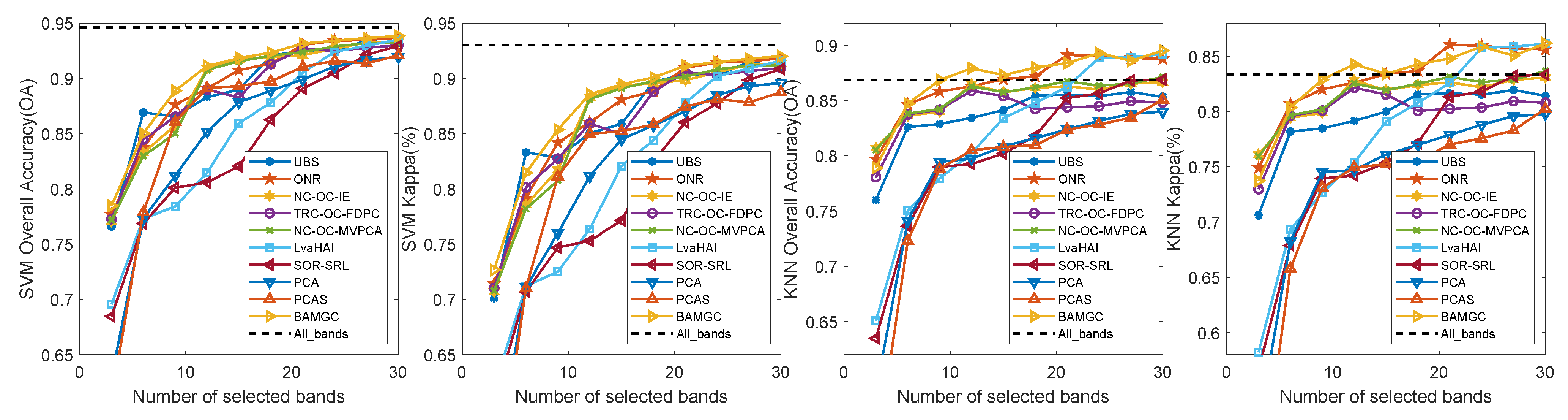
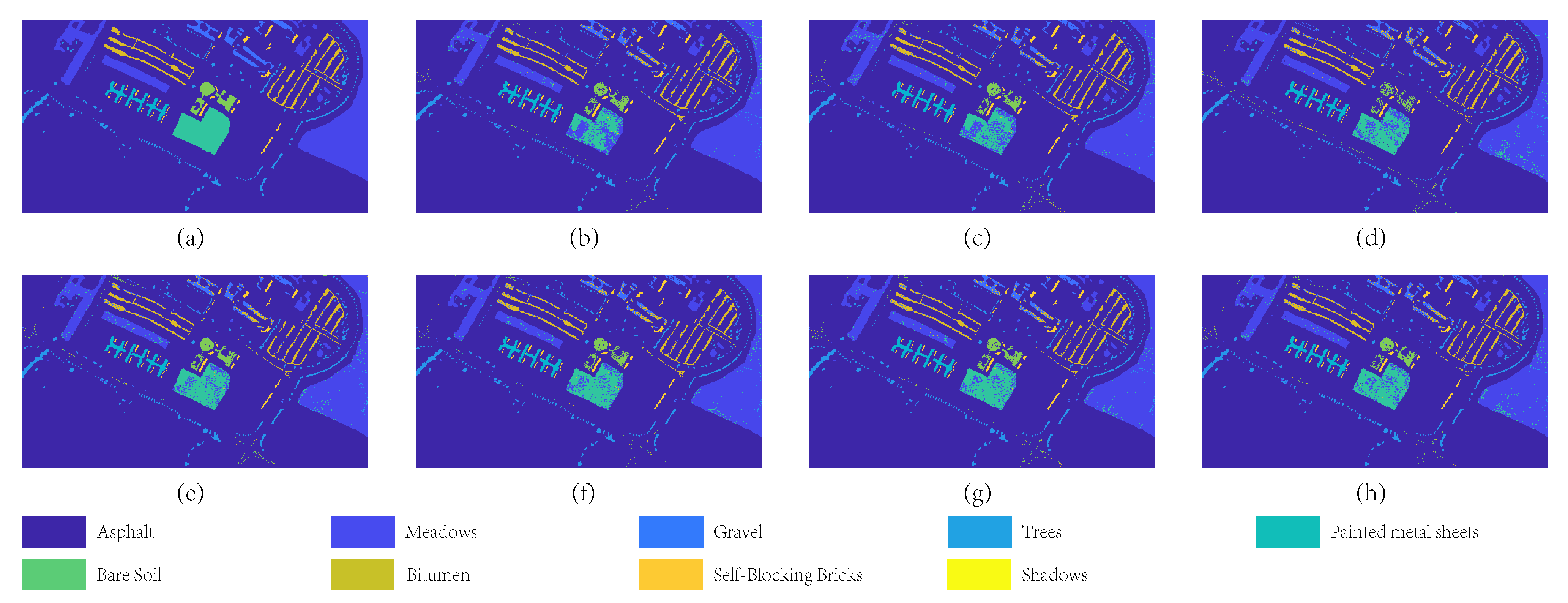
4.4.1. Experimental Results on Pavia University dataset
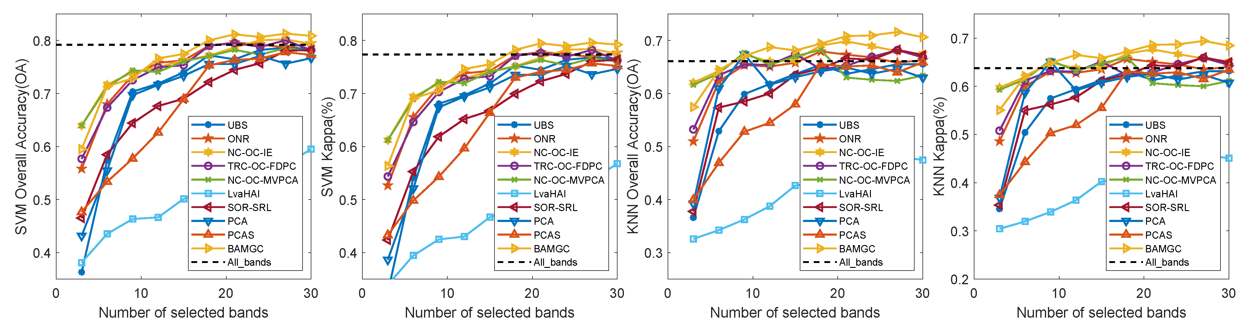
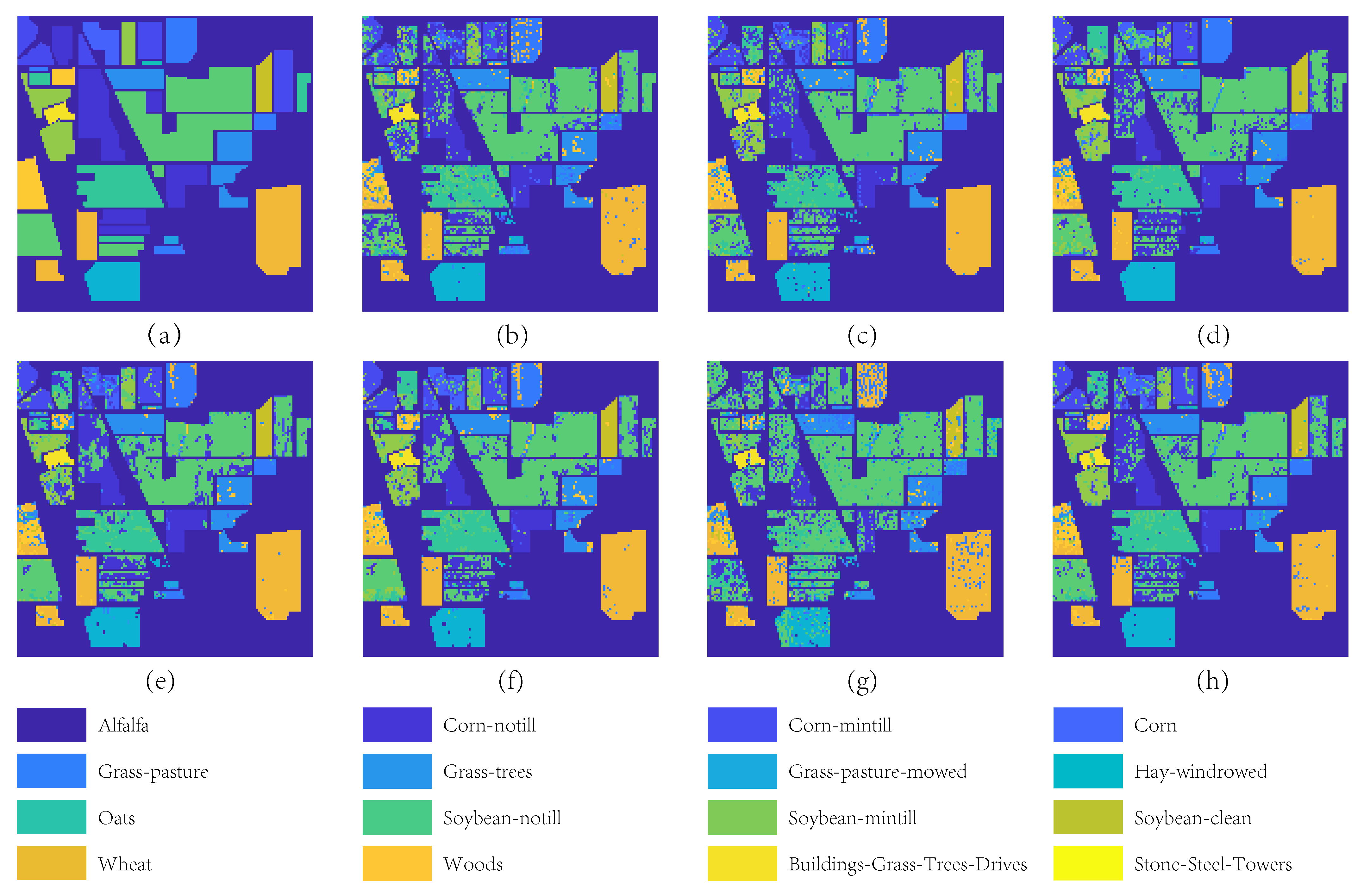
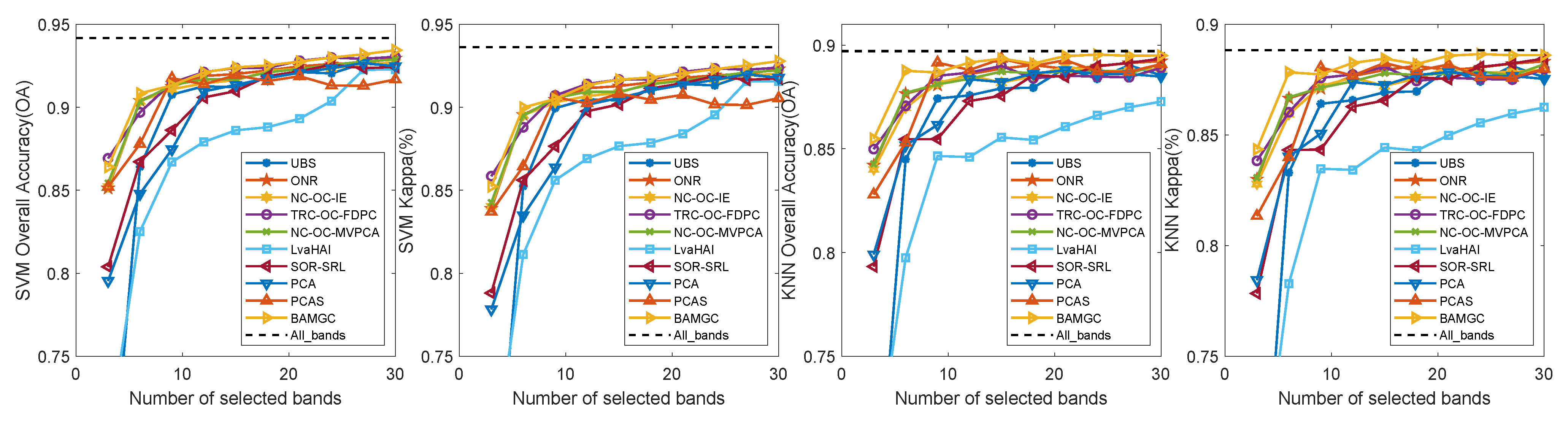
4.4.2. Experimental Results on Indian Pines
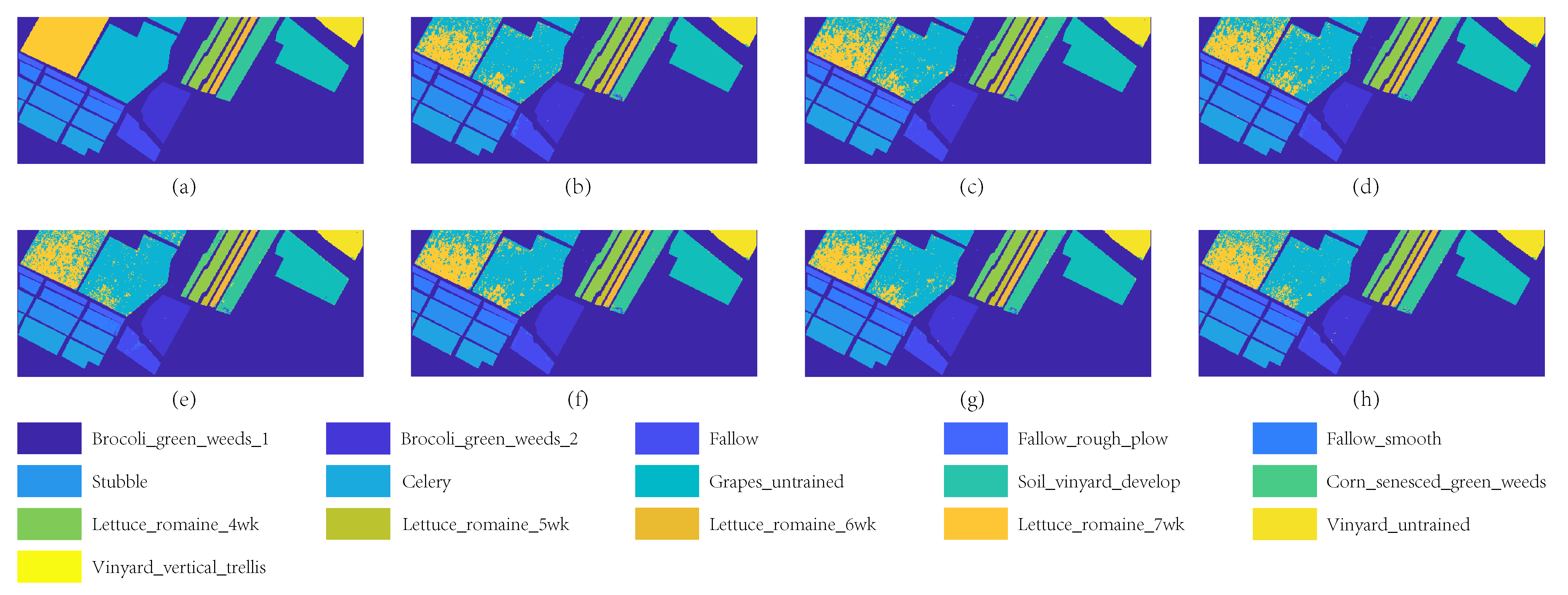
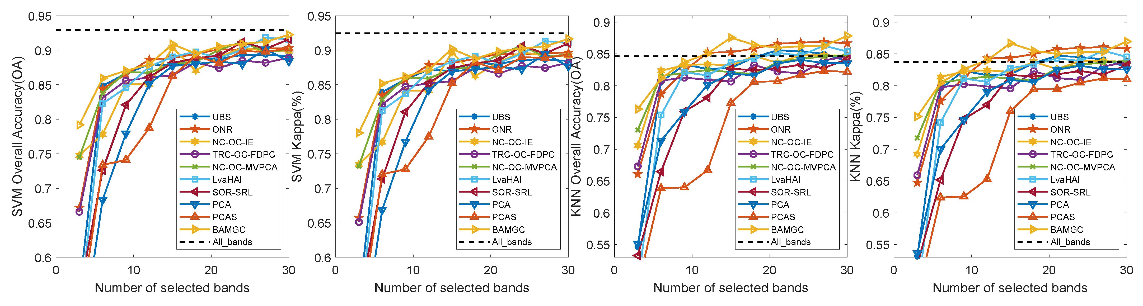
4.4.3. Experimental Results on Salinas
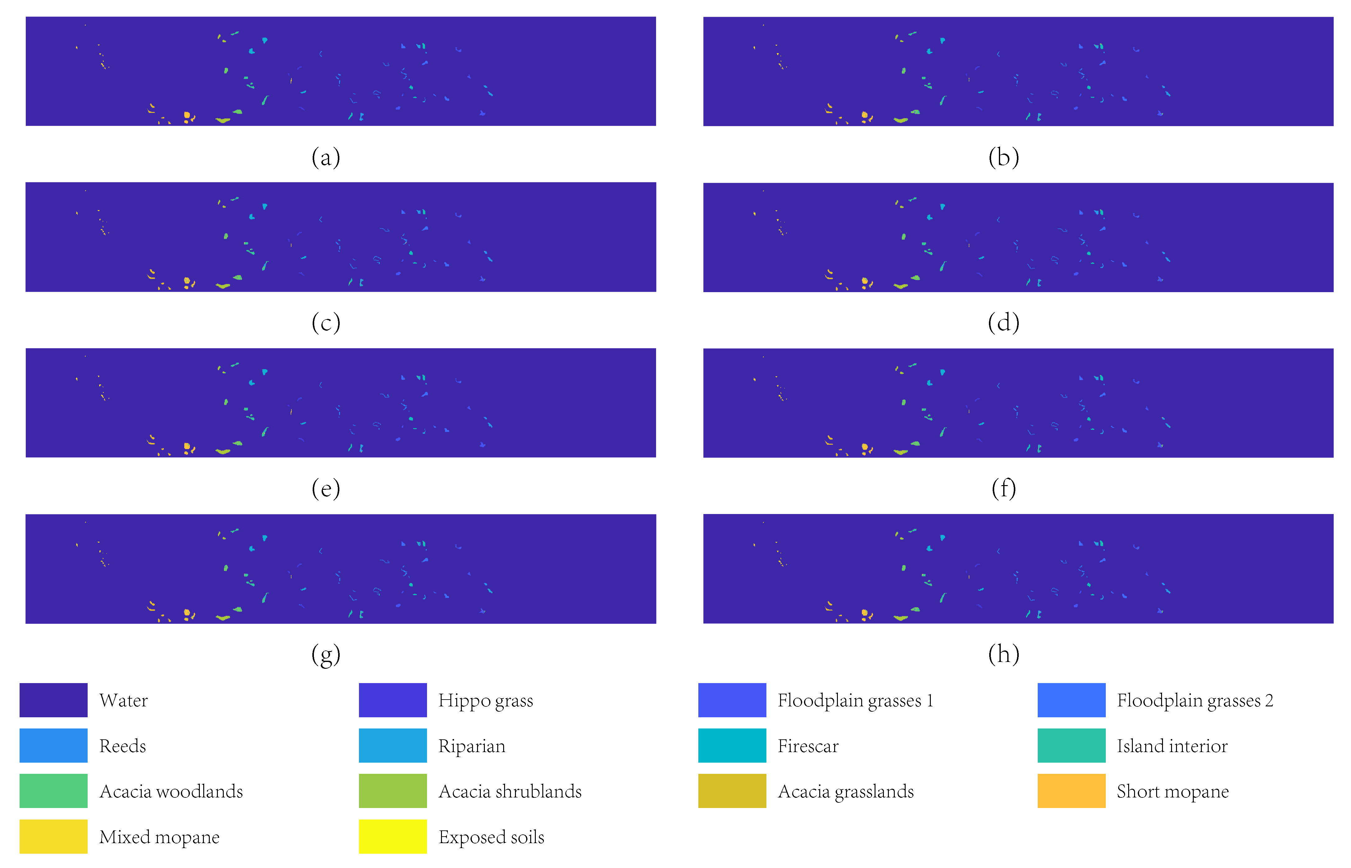
4.4.4. Experimental Results on Botswana Image
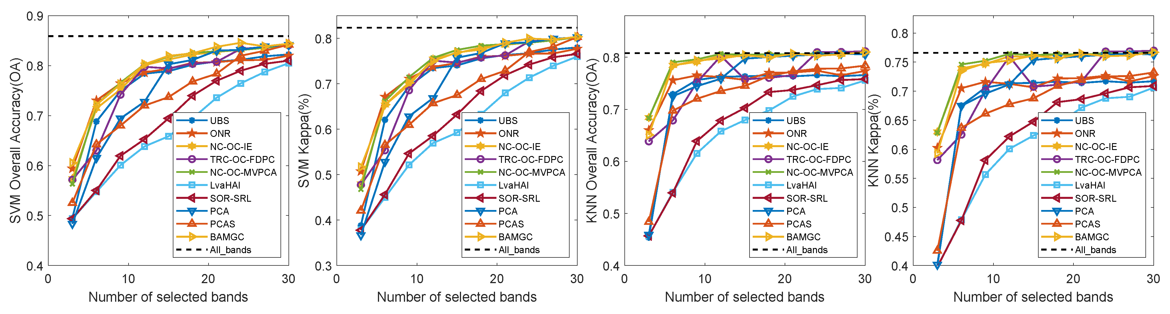
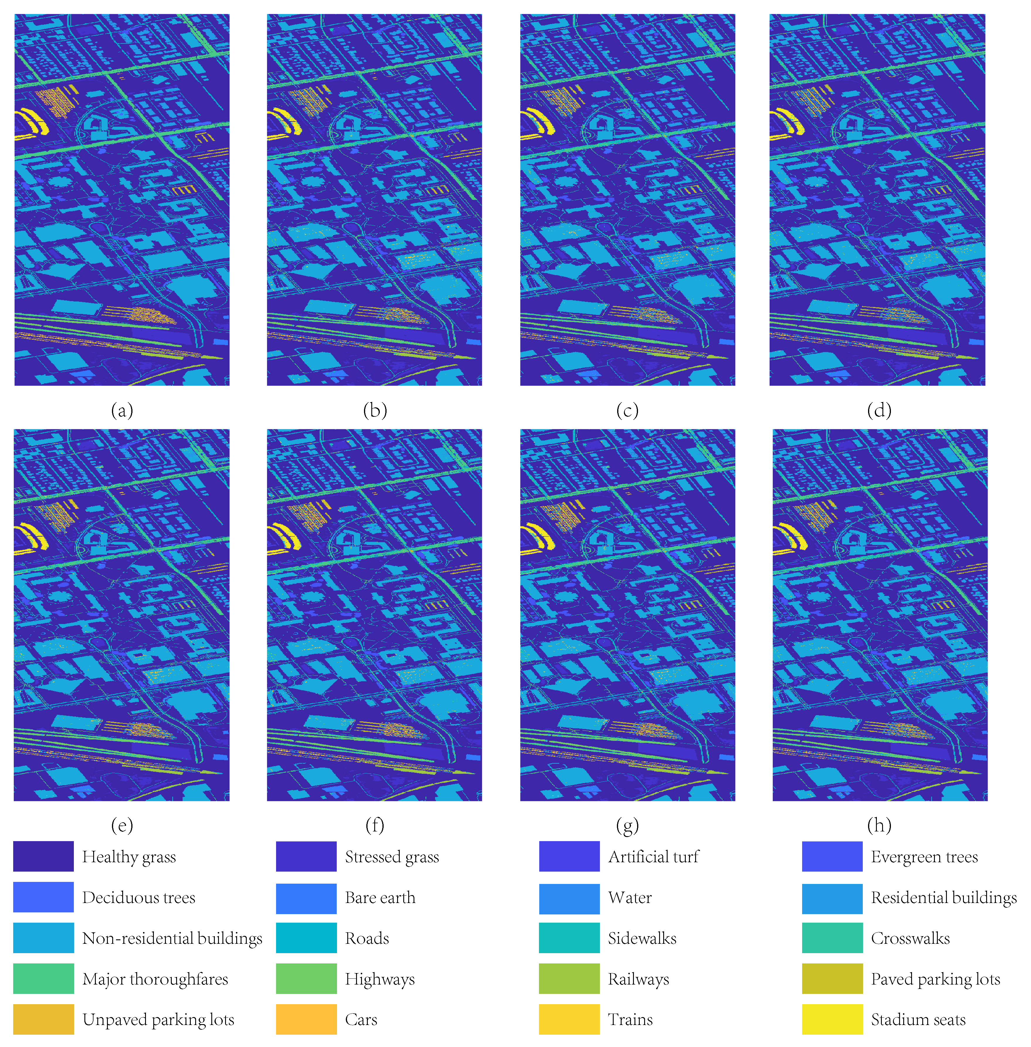
4.4.5. Experimental Results on University of Houston
4.5. Experimental Result Summary
5. Conclusions
Author Contributions
Funding
Data Availability Statement
Conflicts of Interest
References
- Wei, Y.; Zhu, X.; Li, C.; Guo, X.; Yu, X.; Chang, C.; Sun, H. Applications of hyperspectral remote sensing in ground object identification and classification. Adv. Remote Sens. 2017, 6, 201. [Google Scholar] [CrossRef][Green Version]
- Liu, S.; Marinelli, D.; Bruzzone, L.; Bovolo, F. A review of change detection in multitemporal hyperspectral images: Current techniques, applications, and challenges. IEEE Geosci. Remote Sens. Mag. 2019, 7, 140–158. [Google Scholar] [CrossRef]
- Zheng, X.; Gong, T.; Li, X.; Lu, X. Generalized Scene Classification from Small-Scale Datasets with Multitask Learning. IEEE Trans. Geosci. Remote Sens. 2022, 60, 1–11. [Google Scholar] [CrossRef]
- Zhang, Q.; Yuan, Q.; Li, J.; Sun, F.; Zhang, L. Deep spatio-spectral Bayesian posterior for hyperspectral image non-iid noise removal. ISPRS J. Photogramm. Remote Sens. 2020, 164, 125–137. [Google Scholar] [CrossRef]
- Xie, F.; Li, F.; Lei, C.; Yang, J.; Zhang, Y. Unsupervised band selection based on artificial bee colony algorithm for hyperspectral image classification. Appl. Soft Comput. 2019, 75, 428–440. [Google Scholar] [CrossRef]
- Yang, H.; Du, Q.; Chen, G. Unsupervised hyperspectral band selection using graphics processing units. IEEE J. Sel. Top. Appl. Earth Obs. Remote Sens. 2011, 4, 660–668. [Google Scholar] [CrossRef]
- Zheng, X.; Sun, H.; Lu, X.; Xie, W. Rotation-Invariant Attention Network for Hyperspectral Image Classification. IEEE Trans. Image Process. 2022, 31, 4251–4265. [Google Scholar] [CrossRef]
- Feng, J.; Ye, Z.; Liu, S.; Zhang, X.; Chen, J.; Shang, R.; Jiao, L. Dual-graph convolutional network based on band attention and sparse constraint for hyperspectral band selection. Knowl.-Based Syst. 2021, 231, 107428. [Google Scholar] [CrossRef]
- Habermann, M.; Fremont, V.; Shiguemori, E.H. Supervised band selection in hyperspectral images using single-layer neural networks. Int. J. Remote Sens. 2019, 40, 3900–3926. [Google Scholar] [CrossRef]
- Guo, Z.; Bai, X.; Zhang, Z.; Zhou, J. A hypergraph based semi-supervised band selection method for hyperspectral image classification. In Proceedings of the 2013 IEEE International Conference on Image Processing, Melbourne, VIC, Australia, 15–18 September 2013; pp. 3137–3141. [Google Scholar]
- Zheng, X.; Wang, B.; Du, X.; Lu, X. Mutual Attention Inception Network for Remote Sensing Visual Question Answering. IEEE Trans. Geosci. Remote Sens. 2022, 60, 1–14. [Google Scholar] [CrossRef]
- Zhu, G.; Huang, Y.; Lei, J.; Bi, Z.; Xu, F. Unsupervised hyperspectral band selection by dominant set extraction. IEEE Trans. Geosci. Remote Sens. 2015, 54, 227–239. [Google Scholar] [CrossRef]
- Zheng, X.; Chen, X.; Lu, X.; Sun, B. Unsupervised Change Detection by Cross-Resolution Difference Learning. IEEE Trans. Geosci. Remote Sens. 2022, 60, 1–16. [Google Scholar] [CrossRef]
- Yang, C.; Bruzzone, L.; Zhao, H.; Tan, Y.; Guan, R. Superpixel-based unsupervised band selection for classification of hyperspectral images. IEEE Trans. Geosci. Remote Sens. 2018, 56, 7230–7245. [Google Scholar] [CrossRef]
- Gong, M.; Zhang, M.; Yuan, Y. Unsupervised band selection based on evolutionary multiobjective optimization for hyperspectral images. IEEE Trans. Geosci. Remote Sens. 2015, 54, 544–557. [Google Scholar] [CrossRef]
- Jia, S.; Ji, Z.; Qian, Y.; Shen, L. Unsupervised band selection for hyperspectral imagery classification without manual band removal. IEEE J. Sel. Top. Appl. Earth Obs. Remote Sens. 2012, 5, 531–543. [Google Scholar] [CrossRef]
- Tarabalka, Y.; Fauvel, M.; Chanussot, J.; Benediktsson, J.A. SVM-and MRF-based method for accurate classification of hyperspectral images. IEEE Geosci. Remote Sens. Lett. 2010, 7, 736–740. [Google Scholar] [CrossRef]
- Tang, C.; Liu, X.; Zhu, E.; Wang, L.; Zomaya, A. Hyperspectral Band Selection via Spatial-Spectral Weighted Region-wise Multiple Graph Fusion-Based Spectral Clustering. In Proceedings of the Thirtieth International Joint Conference on Artificial Intelligence, Montreal-themed Virtual Reality, 19–27 August 2021; pp. 3038–3344. [Google Scholar]
- Beirami, B.A.; Mokhtarzade, M. An Automatic Method for Unsupervised Feature Selection of Hyperspectral Images Based on Fuzzy Clustering of Bands. Trait. Signal 2020, 37, 319–324. [Google Scholar] [CrossRef]
- Sun, W.; Du, Q. Hyperspectral band selection: A review. IEEE Geosci. Remote Sens. Mag. 2019, 7, 118–139. [Google Scholar] [CrossRef]
- Sun, W.; Du, Q. Graph-regularized fast and robust principal component analysis for hyperspectral band selection. IEEE Trans. Geosci. Remote Sens. 2018, 56, 3185–3195. [Google Scholar] [CrossRef]
- Chang, C.I.; Du, Q. Interference and noise-adjusted principal components analysis. IEEE Trans. Geosci. Remote Sens. 1999, 37, 2387–2396. [Google Scholar] [CrossRef]
- Wang, Q.; Lin, J.; Yuan, Y. Salient band selection for hyperspectral image classification via manifold ranking. IEEE Trans. Neural Netw. Learn. Syst. 2016, 27, 1279–1289. [Google Scholar] [CrossRef]
- Jia, S.; Tang, G.; Zhu, J.; Li, Q. A novel ranking-based clustering approach for hyperspectral band selection. IEEE Trans. Geosci. Remote Sens. 2015, 54, 88–102. [Google Scholar] [CrossRef]
- Wang, Q.; Li, Q.; Li, X. Hyperspectral band selection via adaptive subspace partition strategy. IEEE J. Sel. Top. Appl. Earth Obs. Remote Sens. 2019, 12, 4940–4950. [Google Scholar] [CrossRef]
- Su, H.; Cai, Y.; Du, Q. Firefly-Algorithm-Inspired Framework with Band Selection and Extreme Learning Machine for Hyperspectral Image Classification. IEEE J. Sel. Top. Appl. Earth Obs. Remote Sens. 2017, 10, 309–320. [Google Scholar] [CrossRef]
- Yang, H.; Du, Q.; Chen, G. Particle swarm optimization-based hyperspectral dimensionality reduction for urban land cover classification. IEEE J. Sel. Top. Appl. Earth Obs. Remote Sens. 2012, 5, 544–554. [Google Scholar] [CrossRef]
- Su, H.; Du, Q.; Chen, G.; Du, P. Optimized hyperspectral band selection using particle swarm optimization. IEEE J. Sel. Top. Appl. Earth Obs. Remote Sens. 2014, 7, 2659–2670. [Google Scholar] [CrossRef]
- Yuan, Y.; Zheng, X.; Lu, X. Discovering diverse subset for unsupervised hyperspectral band selection. IEEE Trans. Image Process. 2016, 26, 51–64. [Google Scholar] [CrossRef]
- Zhang, R.; Ma, J. Feature selection for hyperspectral data based on recursive support vector machines. Int. J. Remote Sens. 2009, 30, 3669–3677. [Google Scholar] [CrossRef]
- Zhong, P.; Zhang, P.; Wang, R. Dynamic learning of SMLR for feature selection and classification of hyperspectral data. IEEE Geosci. Remote Sens. Lett. 2008, 5, 280–284. [Google Scholar] [CrossRef]
- Roweis, S.T.; Saul, L.K. Nonlinear dimensionality reduction by locally linear embedding. Science 2000, 290, 2323–2326. [Google Scholar] [CrossRef] [PubMed]
- Belkin, M.; Niyogi, P. Laplacian eigenmaps for dimensionality reduction and data representation. Neural Comput. 2003, 15, 1373–1396. [Google Scholar] [CrossRef]
- He, X.; Cai, D.; Yan, S.; Zhang, H.J. Neighborhood preserving embedding. In Proceedings of the Tenth IEEE International Conference on Computer Vision (ICCV’05) Volume 1, Beijing, China, 17–21 October 2005; Volume 2, pp. 1208–1213. [Google Scholar]
- Li, K.; Luo, G.; Ye, Y.; Li, W.; Ji, S.; Cai, Z. Adversarial privacy-preserving graph embedding against inference attack. IEEE Internet Things J. 2020, 8, 6904–6915. [Google Scholar] [CrossRef]
- Zhong, Z.; Li, J.; Luo, Z.; Chapman, M. Spectral–spatial residual network for hyperspectral image classification: A 3-D deep learning framework. IEEE Trans. Geosci. Remote Sens. 2017, 56, 847–858. [Google Scholar] [CrossRef]
- Islam, M.; Sohaib, M.; Kim, J.; Kim, J.M. Crack Classification of a Pressure Vessel Using Feature Selection and Deep Learning Methods. Sensors 2018, 18, 4379. [Google Scholar] [CrossRef]
- Ribalta Lorenzo, P.; Tulczyjew, L.; Marcinkiewicz, M.; Nalepa, J. Hyperspectral band selection using attention-based convolutional neural networks. IEEE Access 2020, 8, 42384–42403. [Google Scholar] [CrossRef]
- Kang, M.; Kim, J.; Wills, L.M.; Kim, J.M. Time-varying and multiresolution envelope analysis and discriminative feature analysis for bearing fault diagnosis. IEEE Trans. Ind. Electron. 2015, 62, 7749–7761. [Google Scholar] [CrossRef]
- Cai, Y.; Liu, X.; Cai, Z. BS-Nets: An end-to-end framework for band selection of hyperspectral image. IEEE Trans. Geosci. Remote Sens. 2019, 58, 1969–1984. [Google Scholar] [CrossRef]
- Mou, L.; Saha, S.; Hua, Y.; Bovolo, F.; Bruzzone, L.; Zhu, X.X. Deep reinforcement learning for band selection in hyperspectral image classification. IEEE Trans. Geosci. Remote Sens. 2021, 60, 1–14. [Google Scholar] [CrossRef]
- Nie, F.; Zhang, R.; Li, X. A generalized power iteration method for solving quadratic problem on the Stiefel manifold. Sci. Inf. Sci. 2017, 60, 112101. [Google Scholar] [CrossRef]
- Wang, Q.; Zhang, F.; Li, X. Optimal clustering framework for hyperspectral band selection. IEEE Trans. Geosci. Remote Sens. 2018, 56, 5910–5922. [Google Scholar] [CrossRef]
- Stella, X.Y.; Shi, J. Multiclass spectral clustering. In Proceedings of the Computer Vision, IEEE International Conference, Nice, France, 13–16 October 2003; p. 313. [Google Scholar]
- Chang, C.I.; Du, Q.; Sun, T.L.; Althouse, M.L. A joint band prioritization and band-decorrelation approach to band selection for hyperspectral image classification. IEEE Trans. Geosci. Remote Sens. 1999, 37, 2631–2641. [Google Scholar] [CrossRef]
- Wang, Q.; Zhang, F.; Li, X. Hyperspectral band selection via optimal neighborhood reconstruction. IEEE Trans. Geosci. Remote Sens. 2020, 58, 8465–8476. [Google Scholar] [CrossRef]
- Wei, X.; Cai, L.; Liao, B.; Lu, T. Local-View-Assisted Discriminative Band Selection with Hypergraph Autolearning for Hyperspectral Image Classification. IEEE Trans. Geosci. Remote Sens. 2019, 58, 2042–2055. [Google Scholar] [CrossRef]
- Wei, X.; Zhu, W.; Liao, B.; Cai, L. Scalable one-pass self-representation learning for hyperspectral band selection. IEEE Trans. Geosci. Remote Sens. 2019, 57, 4360–4374. [Google Scholar] [CrossRef]
- Zabalza, J.; Ren, J.; Ren, J.; Liu, Z.; Marshall, S. Structured covariance principal component analysis for real-time onsite feature extraction and dimensionality reduction in hyperspectral imaging. Appl. Opt. 2014, 53, 4440–4449. [Google Scholar] [CrossRef] [PubMed]


| Method | Pros | Cons |
|---|---|---|
| MVPCA | All bands are ranked by the variance of band capacity. | Redundancy of band information is not considered. |
| UBS | Using divergence based on the analysis of band features, it tries to solve the redundancy problem caused by sorting algorithm. | The spatial information of HSI is not considered. |
| FDPC | It is a clustering method based on weighted normalized local density and ranking. | The selected bands do not necessarily contain the most information, and different metrics will affect the results. Moreover, the random initialization of the clustering algorithm is uncertain. |
| FA | FA can reduce the complexity of the ELM (extreme learning machine) network, and is suitable for optimizing the parameters in the network. It converges faster compared with PSO. | It is sensitive to parameters and will be less attractive when the dimension is high, affecting the result update. |
| PSO | It is a probabilistic global optimization algorithm that is relatively simple and easier to implement. | Its peak seeking rate and solution accuracy are low. |
| ABA (Attention-Based Autoencoders) | This method presents an automatic encoder based on an attention mechanism to realize the non-linear relationship between bands. | The optimization process of its hyperparameters is random, which leads to the instability of the model. |
| ABCNN (Attention-Based Convolutional Neural Networks) | This method attains the optimal subset of bands by coupling attention-based CNNs with anomaly detection. | Deep learning incorporating an attention mechanism is prone to over-fitting. |
| DRL (Deep Reinforcement Learning) | It is a deep learning method for environment simulation that makes full use of hyperspectral sequence to select bands. | Since this is an algorithm based on deep learning, it takes more time to train. |
| BS-Nets | It proposes a deep learning method combined with an attention mechanism and rebuilding RecNet. The framework is flexible and can adapt to more existing networks. | Models need a long time to be trained. |
| Parameter | Pavia University | Indian Pines | Salinas | Botswana | University of Houston |
|---|---|---|---|---|---|
| C | 10,000.0 | 100.0 | 100.0 | 10,000.0 | 10,000.0 |
| gamma | 0.5 | 4.0 | 16.0 | 0.5 | 0.5 |
| Dataset | Method | SVM | KNN | ||
|---|---|---|---|---|---|
| OA | OA | ||||
| Pavia University | UBS | 89.00 | 85.89 | 84.14 | 80.00 |
| ONR | 90.75 | 88.08 | 86.93 | 83.38 | |
| NC-OC-IE | 91.73 | 89.34 | 85.74 | 81.92 | |
| TRC-OC-FDPC | 88.28 | 84.93 | 85.40 | 81.54 | |
| NC-OC-MVPCA | 91.55 | 89.11 | 85.75 | 81.94 | |
| LvaHAI | 85.97 | 82.08 | 83.40 | 79.09 | |
| SOR-SRL | 82.05 | 77.16 | 80.19 | 75.35 | |
| PCA | 87.85 | 84.49 | 80.85 | 76.11 | |
| PCAS | 89.32 | 85.23 | 80.80 | 75.23 | |
| BAMGC | 91.83 | 89.46 | 87.29 | 83.41 | |
| Indian Pines | UBS | 73.99 | 71.91 | 63.67 | 61.29 |
| ONR | 76.24 | 74.29 | 65.81 | 63.53 | |
| NC-OC-IE | 76.26 | 74.20 | 66.31 | 63.96 | |
| TRC-OC-FDPC | 75.34 | 73.26 | 67.47 | 65.14 | |
| NC-OC-MVPCA | 76.10 | 74.10 | 67.02 | 64.76 | |
| LvaHAI | 50.14 | 46.66 | 42.66 | 40.24 | |
| SOR-SRL | 69.03 | 66.76 | 63.54 | 61.17 | |
| PCA | 73.34 | 71.17 | 63.08 | 60.76 | |
| PCAS | 68.95 | 66.39 | 57.97 | 55.51 | |
| BAMGC | 77.47 | 75.52 | 68.13 | 65.84 | |
| Salinas | UBS | 91.20 | 90.42 | 87.92 | 86.93 |
| ONR | 92.01 | 91.28 | 88.86 | 87.94 | |
| NC-OC-IE | 91.63 | 90.88 | 88.19 | 87.22 | |
| TRC-OC-FDPC | 92.37 | 91.67 | 88.99 | 88.08 | |
| NC-OC-MVPCA | 91.68 | 90.93 | 88.72 | 87.79 | |
| LvaHAI | 88.61 | 87.66 | 85.55 | 84.43 | |
| SOR-SRL | 90.98 | 90.18 | 87.56 | 86.56 | |
| PCA | 91.35 | 90.57 | 88.21 | 87.25 | |
| PCAS | 91.94 | 90.83 | 89.33 | 88.25 | |
| BAMGC | 92.41 | 91.67 | 89.35 | 88.45 | |
| Botswana | UBS | 87.78 | 87.01 | 82.76 | 81.78 |
| ONR | 88.87 | 88.15 | 85.26 | 84.35 | |
| NC-OC-IE | 90.34 | 89.69 | 83.14 | 82.16 | |
| TRC-OC-FDPC | 86.35 | 85.51 | 80.65 | 79.57 | |
| NC-OC-MVPCA | 88.05 | 87.29 | 82.12 | 81.09 | |
| LvaHAI | 89.03 | 88.37 | 83.66 | 82.74 | |
| SOR-SRL | 88.16 | 87.40 | 82.66 | 81.67 | |
| PCA | 87.71 | 86.93 | 81.91 | 80.89 | |
| PCAS | 86.25 | 85.22 | 77.27 | 75.99 | |
| BAMGC | 90.87 | 90.19 | 87.55 | 86.66 | |
| Houston | UBS | 78.89 | 74.04 | 76.34 | 71.44 |
| ONR | 79.38 | 74.59 | 75.66 | 70.66 | |
| NC-OC-IE | 81.22 | 76.76 | 80.21 | 75.91 | |
| TRC-OC-FDPC | 79.43 | 74.66 | 75.77 | 70.77 | |
| NC-OC-MVPCA | 81.77 | 77.45 | 80.46 | 76.20 | |
| LvaHAI | 65.85 | 59.25 | 67.94 | 62.37 | |
| SOR-SRL | 69.45 | 63.25 | 70.28 | 64.75 | |
| PCA | 80.26 | 75.74 | 79.73 | 75.37 | |
| PCAS | 73.69 | 67.52 | 74.49 | 68.77 | |
| BAMGC | 81.95 | 76.91 | 80.43 | 76.14 | |
| Dataset | Method | SVM | KNN | ||
|---|---|---|---|---|---|
| OA | OA | ||||
| Pavia University | UBS | 93.41 | 91.46 | 85.77 | 81.95 |
| ONR | 93.69 | 91.81 | 89.12 | 86.06 | |
| NC-OC-IE | 93.33 | 91.36 | 86.67 | 83.08 | |
| TRC-OC-FDPC | 93.00 | 90.93 | 85.89 | 82.15 | |
| NC-OC-MVPCA | 93.19 | 91.20 | 87.14 | 83.66 | |
| LvaHAI | 93.52 | 91.60 | 89.18 | 86.14 | |
| SOR-SRL | 92.93 | 90.86 | 86.90 | 83.34 | |
| PCA | 91.93 | 89.59 | 83.99 | 79.76 | |
| PCAS | 92.08 | 88.75 | 85.08 | 80.27 | |
| BAMGC | 93.84 | 92.02 | 89.51 | 86.16 | |
| Indian Pines | UBS | 78.66 | 76.79 | 65.54 | 63.16 |
| ONR | 79.63 | 77.83 | 67.94 | 65.71 | |
| NC-OC-IE | 80.21 | 78.40 | 69.85 | 67.66 | |
| TRC-OC-FDPC | 80.05 | 78.22 | 68.19 | 65.89 | |
| NC-OC-MVPCA | 78.55 | 76.66 | 68.25 | 65.97 | |
| LvaHAI | 59.51 | 56.77 | 48.15 | 45.82 | |
| SOR-SRL | 78.19 | 76.39 | 68.26 | 66.00 | |
| PCA | 77.11 | 75.18 | 67.38 | 65.10 | |
| PCAS | 77.82 | 75.69 | 65.89 | 63.44 | |
| BAMGC | 81.29 | 79.61 | 71.61 | 69.42 | |
| Salinas | UBS | 92.64 | 91.96 | 89.02 | 88.11 |
| ONR | 92.95 | 92.29 | 89.23 | 88.33 | |
| NC-OC-IE | 92.70 | 92.02 | 88.96 | 88.04 | |
| TRC-OC-FDPC | 93.04 | 92.39 | 88.99 | 88.08 | |
| NC-OC-MVPCA | 92.88 | 92.23 | 89.10 | 88.20 | |
| LvaHAI | 92.27 | 91.57 | 87.28 | 86.25 | |
| SOR-SRL | 92.57 | 91.88 | 89.35 | 88.45 | |
| PCA | 92.67 | 92.00 | 88.78 | 87.85 | |
| PCAS | 91.94 | 90.83 | 89.33 | 88.25 | |
| BAMGC | 93.44 | 92.78 | 89.54 | 88.66 | |
| Botswana | UBS | 89.35 | 88.65 | 85.56 | 84.68 |
| ONR | 90.31 | 89.66 | 86.89 | 86.07 | |
| NC-OC-IE | 90.34 | 89.69 | 84.78 | 83.87 | |
| TRC-OC-FDPC | 88.91 | 88.18 | 84.61 | 83.69 | |
| NC-OC-MVPCA | 91.23 | 90.63 | 84.81 | 83.91 | |
| LvaHAI | 91.84 | 91.33 | 86.30 | 85.49 | |
| SOR-SRL | 91.57 | 90.99 | 84.16 | 83.22 | |
| PCA | 90.14 | 89.48 | 84.06 | 83.12 | |
| PCAS | 90.23 | 89.37 | 82.31 | 81.14 | |
| BAMGC | 92.24 | 91.64 | 87.83 | 86.96 | |
| Houston | UBS | 82.24 | 78.00 | 76.59 | 71.72 |
| ONR | 82.01 | 77.72 | 77.42 | 72.65 | |
| NC-OC-IE | 84.16 | 80.27 | 80.96 | 76.75 | |
| TRC-OC-FDPC | 84.06 | 80.15 | 81.15 | 76.97 | |
| NC-OC-MVPCA | 84.14 | 80.25 | 80.99 | 76.79 | |
| LvaHAI | 80.49 | 75.99 | 75.56 | 70.62 | |
| SOR-SRL | 81.00 | 76.58 | 75.82 | 70.90 | |
| PCA | 84.13 | 80.23 | 80.70 | 76.48 | |
| PCAS | 84.20 | 80.29 | 78.40 | 73.22 | |
| BAMGC | 84.56 | 80.34 | 81.00 | 76.69 | |
| Pavia University | Indian Pines | Salinas | Botswana | University of Houston | Mean Value | |
|---|---|---|---|---|---|---|
| LvaHAI | 84.99 | 50.26 | 86.87 | 84.74 | 67.26 | 74.83 |
| SOR-SRL | 83.90 | 68.47 | 89.87 | 83.46 | 69.24 | 78.99 |
| PCAS | 85.91 | 67.37 | 90.58 | 81.03 | 73.48 | 79.67 |
| PCA | 84.79 | 69.38 | 89.54 | 80.75 | 74.76 | 79.85 |
| UBS | 89.10 | 69.89 | 88.50 | 84.77 | 75.68 | 81.59 |
| TRC-OC-FDPC | 88.78 | 74.34 | 91.67 | 84.89 | 76.58 | 83.25 |
| ONR | 89.38 | 74.54 | 91.36 | 86.58 | 77.23 | 83.82 |
| NC-OC-IE | 89.20 | 75.63 | 91.19 | 85.92 | 78.12 | 84.01 |
| NC-OC-MVPCA | 89.12 | 74.89 | 91.31 | 86.94 | 78.33 | 84.12 |
| BAMGC | 90.17 | 76.19 | 91.80 | 88.54 | 79.02 | 85.14 |
Publisher’s Note: MDPI stays neutral with regard to jurisdictional claims in published maps and institutional affiliations. |
© 2022 by the authors. Licensee MDPI, Basel, Switzerland. This article is an open access article distributed under the terms and conditions of the Creative Commons Attribution (CC BY) license (https://creativecommons.org/licenses/by/4.0/).
Share and Cite
You, M.; Meng, X.; Wang, Y.; Jin, H.; Zhai, C.; Yuan, A. Hyperspectral Band Selection via Band Grouping and Adaptive Multi-Graph Constraint. Remote Sens. 2022, 14, 4379. https://doi.org/10.3390/rs14174379
You M, Meng X, Wang Y, Jin H, Zhai C, Yuan A. Hyperspectral Band Selection via Band Grouping and Adaptive Multi-Graph Constraint. Remote Sensing. 2022; 14(17):4379. https://doi.org/10.3390/rs14174379
Chicago/Turabian StyleYou, Mengbo, Xiancheng Meng, Yishu Wang, Hongyuan Jin, Chunting Zhai, and Aihong Yuan. 2022. "Hyperspectral Band Selection via Band Grouping and Adaptive Multi-Graph Constraint" Remote Sensing 14, no. 17: 4379. https://doi.org/10.3390/rs14174379
APA StyleYou, M., Meng, X., Wang, Y., Jin, H., Zhai, C., & Yuan, A. (2022). Hyperspectral Band Selection via Band Grouping and Adaptive Multi-Graph Constraint. Remote Sensing, 14(17), 4379. https://doi.org/10.3390/rs14174379