
Wavelet-Domain Information-Hiding Technology with High-Quality Audio Signals on MEMS Sensors

Abstract
1. Introduction
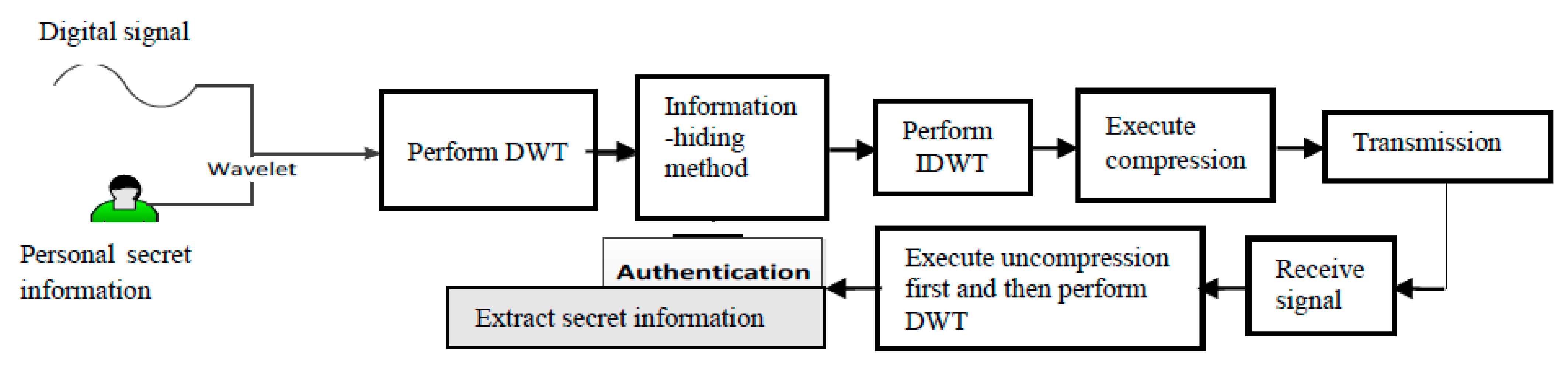
2. Proposed Method
2.1. Embedding Technique
- If the bit “” is embedded into , then is quantized by(b) Compression constraint;
- If the bit “” is embedded into , then is quantized by(b) Compression constraint;
2.2. Compression Constraint
3. Proposed Optimization Solution in Embedding and Extraction Method
3.1. First Step in Finding the Optimal Solution
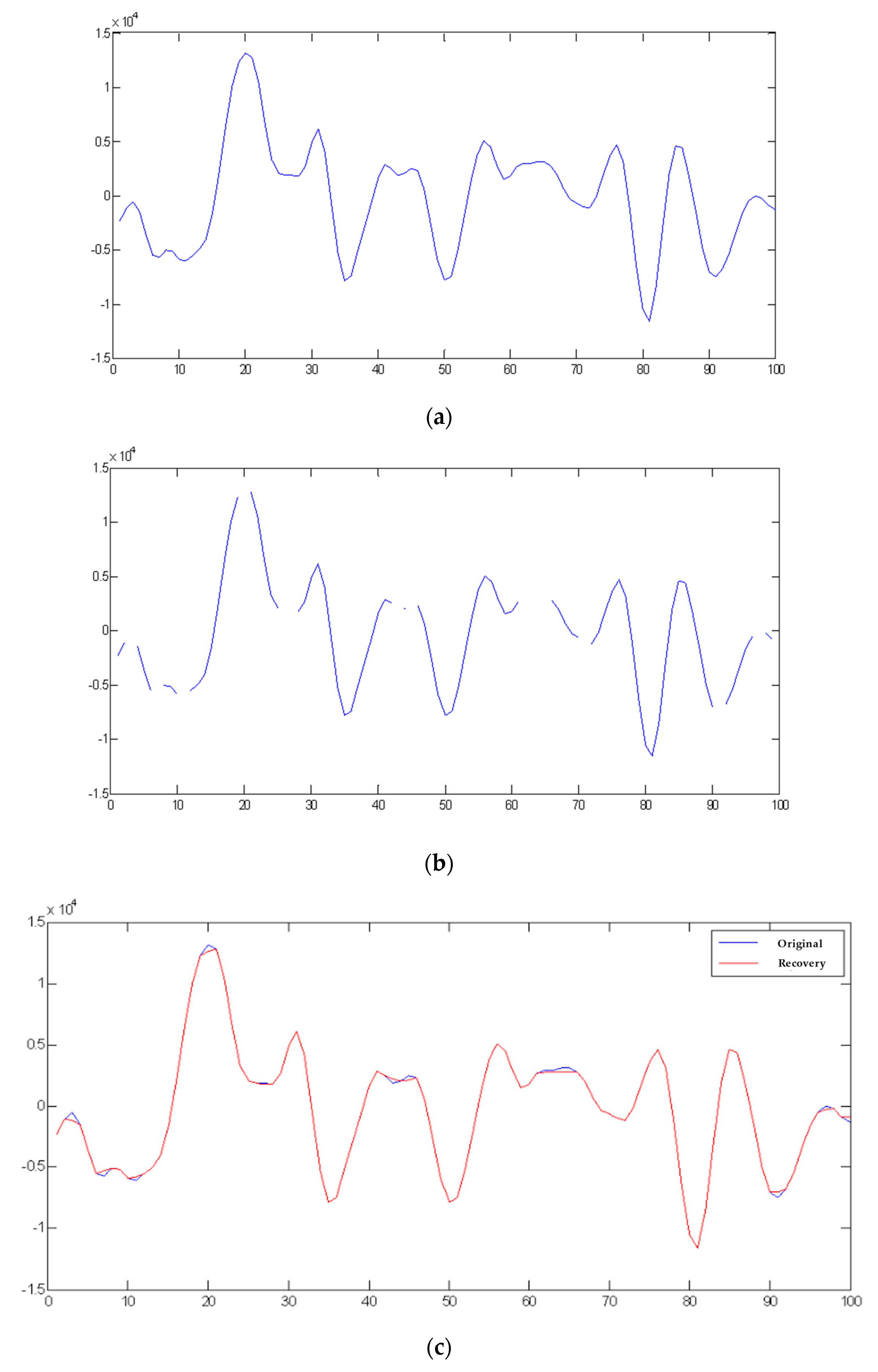
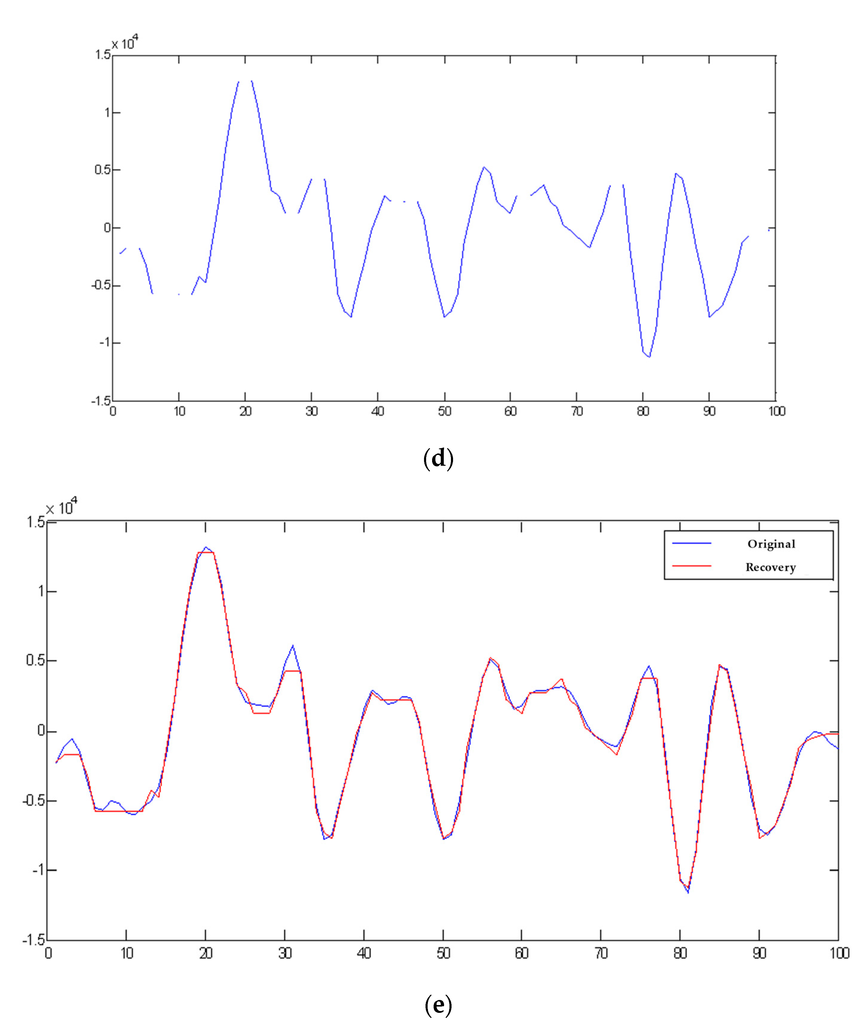
3.2. Audio Recovery and Information Extraction
- If
- If
3.3. Application Scenarios of Our Proposal
4. Experimental Results
4.1. Embedding Capacity and Averaged SNR
4.2. Robustness Measurement
- (1)
- Re-sampling: In the re-sampling process, the sampling rate of an audio signal can be increased (up-sample) or decreased (down-sample) in three stages: (i) down-sample, (ii) interpolation, and (iii) up-sample. We down-sampled the sampling rate of embedded audios from 44.1 kHz to 22.05 kHz, then up-sampled them from 22.05 kHz back to 44.1 kHz with a linear interpolation filter. A similar approach allowed the sampling rates to change from 44.1 kHz to 11.025 kHz and 8 kHz and regain the original rate of 44.1 kHz. Table 2 shows the BER of testing re-sampling on audio signals. One can see that when the re-sampling rate is 8 kHz, the proposed embedding method has lower BER than those from implementations in [24,27]. In those cases when the re-sampling rates are 22.05 kHz and 11.025 kHz, the proposed method shows comparable robustness.
- (2)
- Low-pass filtering: Table 3 presents the BER while testing low-pass filters with cutoff frequencies of 3 kHz and 5 kHz. The BER results show that models in [24,27] have slightly higher robustness. Since both references [24,27] also adopted quantization-based embedding technique, the BER evaluation of the proposed method gives extremely similar results to theirs during the process of low-pass filtering.
- (3)
- (4)
- Amplitude scaling: Since the amplitude-scaling attack usually results in saturation, in this study, we selected four distinct values for the amplitude-scaling factor: 0.5, 0.8, 1.1, and 1.2. The experimental results in Table 5 confirm that the proposed algorithm is much more robust than the methods in references [24,27].
- (5)
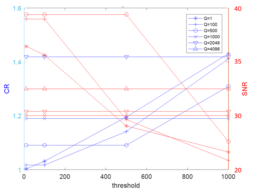
4.3. Compression Measurement
5. Conclusions
Author Contributions
Funding
Institutional Review Board Statement
Informed Consent Statement
Data Availability Statement
Conflicts of Interest
Appendix A
References
- Chang, C.-L.; Chang, C.-Y.; Tang, Z.-Y.; Chen, S.-T. High-Efficiency Automatic Recharging Mechanism for Cleaning Robot Using Multi-Sensor. Sensors 2018, 18, 11. [Google Scholar] [CrossRef] [PubMed]
- Chang, C.-L.; Chen, C.-J.; Lee, H.-T.; Chang, C.-Y.; Chen, S.-T. Bounding the Sensing Data Collection Time with Ring-based Routing for Industrial Wireless Sensor Networks. J. Internet Technol. 2020, 21, 673–680. [Google Scholar]
- Zuo, Z.; Liu, L.; Zhang, L.; Fang, Y. Indoor Positioning Based on Bluetooth Low-Energy Beacons Adopting Graph Optimization. Sensors 2018, 18, 3736. [Google Scholar] [CrossRef]
- Chang, C.-L.; Chen, S.-T.; Chang, C.-Y.; Jhou, Y.-C. The Application of Machine Learning in Air Hockey Interactive Control System. Sensors 2020, 18, 7233. [Google Scholar] [CrossRef]
- Lin, S.-J.; Chen, S.-T. Enhance the perception of easy-to-fall and apply the Internet of Things to fall prediction and protection. J. Healthc. Commun. 2020, 5, 52. [Google Scholar]
- Zhang, X.; Zhang, S.; Huai, S. Low-Power Indoor Positioning Algorithm Based on iBeacon Network. Hindawi Complex. 2021, 2021, 8475339. [Google Scholar] [CrossRef]
- Zhou, C.; Yuan, J.; Liu, H.; Qiu, J. Bluetooth indoor positioning based on RSSI and Kalman filter. Wirel. Pers. Commun. 2017, 96, 4115–4130. [Google Scholar] [CrossRef]
- Song, W.; Lee, H.M.; Lee, S.H.; Choi, M.H.; Hong, M. Implementation of android application for indoor positioning system with estimote BLE beacons. J. Internet Technol. 2018, 19, 871–878. [Google Scholar]
- Cui, L.; Yang, S.; Chen, F.; Ming, Z.; Lu, N.; Qin, J. A survey on application of machine learning for Internet of Things. Int. J. Mach. Learn. Cyber. 2018, 9, 1399–1417. [Google Scholar] [CrossRef]
- Baldini, G.; Dimc, F.; Kamnik, R.; Steri, G.; Giuliani, R.; Gentile, C. Identification of mobile phones using the built-in magnetometers stimulated by motion patterns. Sensors 2017, 17, 783. [Google Scholar] [CrossRef]
- IFPI (International Federation of the Phonographic Industry). Available online: http://www.ifpi.org (accessed on 10 January 2021).
- Katzenbeisser, S.; Petitcolas, F.A.P. (Eds.) Information Hiding Techniques for Steganography and Digital Watermarking; Artech House, Inc.: Norwood, MA, USA, 2000. [Google Scholar]
- Al-Haj, A.; Mohammad, A.A.; Bata, L. DWT-based audio watermarking. Int. Arab. J. Inf. Technol. 2011, 8, 326–333. [Google Scholar]
- Xiang, S. Robust audio watermarking against the D/A and A/D conversions. EURASIP J. Adv. Signal Processing 2011, 3, 29. [Google Scholar] [CrossRef]
- Chen, S.-T.; Wu, G.-D.; Huang, H.-N. Wavelet-Domain Audio Watermarking Scheme Using Optimization-Based Quantization. IET Signal Processing 2010, 4, 720–727. [Google Scholar] [CrossRef]
- Noriega, R.M.; Nakano, M.; Kurkoski, B.; Yamaguchi, K. High Payload Audio Watermarking: Toward Channel Characterization of MP3 Compression. J. Inf. Hiding Multimed. Signal Process. 2011, 2, 91–107. [Google Scholar]
- Mishra, J.; Patil, M.V.; Chitode, J.S. An Effective Audio Watermarking using DWT-SVD. Int. J. Comput. Appl. 2013, 70, 6–11. [Google Scholar] [CrossRef]
- Zhao, M.; Pan, J.-S.; Chen, S.-T. Entropy-Based Audio Watermarking via the Point of View on the Compact Particle Swarm Optimization. J. Internet Technol. 2015, 16, 485–495. [Google Scholar]
- Darabkh, A.K. Imperceptible and Robust DWT-SVD-Based Digital Audio Watermarking Algorithm. J. Softw. Eng. Appl. 2014, 7, 859–871. [Google Scholar] [CrossRef]
- Chen, S.-T.; Guo, Y.-J.; Huang, H.-N.; Kung, W.-M.; Tseng, K.-K.; Tu, S.-Y. Hiding Patients Confidential Data in the ECG Signal via a Transform-Domain Quantization Scheme. J. Med. Syst. 2014, 38, 54. [Google Scholar] [CrossRef]
- Zear, A.; Singh, A.K.; Kumar, P. A proposed secure multiple watermarking technique based on DWT, DCT and SVD for application in medicine. Multimed. Tools Appl. 2016, 77, 4863–4882. [Google Scholar] [CrossRef]
- Wu, Q.; Wu, M. A Novel Robust Audio Watermarking Algorithm by Modifying the Average Amplitude in Transform Domain. Appl. Sci. 2018, 8, 723. [Google Scholar] [CrossRef]
- Karajeh, H.; Khatib, T.; Rajab, L.; Maqableh, M. A robust digital audio watermarking scheme based on DWT and Schur decomposition. Multimed. Tools Appl. 2019, 78, 18395–18418. [Google Scholar] [CrossRef]
- Chen, S.-T.; Huang, H.-N. Optimization-Based Audio Watermarking with Integrated Quantization Embedding. Multimed. Tools Appl. 2016, 75, 4735–4751. [Google Scholar] [CrossRef]
- Shankar, T.; Yamuna, G. Optimization Based Audio Watermarking using Discrete Wavelet Transform and Singular Value Decomposition. Int. J. Electron. Electr. Comput. Syst. 2017, 6, 375–379. [Google Scholar]
- Dhar, P.K.; Shimamura, T. Blind Audio Watermarking in Transform Domain Based on Singular Value Decomposition and Exponential-Log Operations. Radio Eng. 2017, 26, 552–561. [Google Scholar] [CrossRef]
- Li, J.-F.; Wang, H.-X.; Wu, T.; Sun, X.-M.; Qian, Q. Norm ratio-based audio watermarking scheme in DWT domain. Multimed. Tools Appl. 2018, 77, 14481–14497. [Google Scholar] [CrossRef]
- Mallat, S. A theory for multiresolution signal decomposition: The wavelet representation. IEEE Trans. Pattern Anal. Mach. Intel. 1989, 11, 674–693. [Google Scholar] [CrossRef]
- Burrus, C.S.; Gopinath, R.A.; Gao, H. Introduction to Wavelet Theory and Its Application; Prentice-Hall: Hoboken, NJ, USA, 1998. [Google Scholar]
- Lewis, F.L. Optimal Control; John Wiley and Sons: New York, NY, USA, 1986. [Google Scholar]
- Bartle, R.G. The Elements of Real Analysis, 2nd ed.; Wiley: New York, NY, USA, 1976. [Google Scholar]


| Number of Consecutive Coefficients in DWT Level 8 | Embedding Capacity (bits/11.6 s) | Averaged SNR (dB) | ||||
|---|---|---|---|---|---|---|
| Dance | Love Song | Folklore | Symphony | |||
| Reference [24] | n = 2 | 1000 | 35.8 | 33.4 | 27.9 | 26.3 |
| n = 4 | 500 | 37.7 | 33.5 | 28.6 | 26.2 | |
| Reference [27] | n = 2 | 1000 | 24.3 | 25.4 | 23.2 | 22.3 |
| n = 4 | 500 | 24.1 | 26.0 | 23.6 | 22.9 | |
| Proposed Method | n = 2 | 1000 | 38.3 | 35.6 | 28.7 | 27.5 |
| n = 4 | 500 | 37.1 | 41.3 | 34.5 | 33.2 | |
| Audio Type | Dance | Folklore | Love Song | Symphony | ||||||||||
|---|---|---|---|---|---|---|---|---|---|---|---|---|---|---|
| Re-Sampling Rate (kHz) | 22.05 | 11.025 | 8 | 22.05 | 11.025 | 8 | 22.05 | 11.025 | 8 | 22.05 | 11.025 | 8 | ||
| Reference [24] | n = 2 | mean | 8.32 | 13.31 | 14.01 | 0.74 | 4.22 | 4.36 | 5.74 | 3.08 | 2.39 | 0.78 | 4.52 | 4.76 |
| SD | 0.40 | 0.43 | 0.41 | 0.23 | 0.28 | 0.26 | 0.16 | 0.15 | 0.16 | 0.16 | 0.26 | 0.28 | ||
| n = 4 | mean | 2.36 | 8.01 | 8.01 | 0.20 | 1.24 | 1.26 | 0.72 | 1.05 | 1.06 | 0.32 | 1.29 | 1.29 | |
| SD | 0.25 | 0.38 | 0.36 | 0.18 | 0.21 | 0.19 | 0.10 | 0.12 | 0.12 | 0.13 | 0.21 | 0.21 | ||
| Reference [27] | mean | 9.14 | 15.26 | 15.31 | 0.74 | 4.22 | 4.36 | 5.74 | 3.08 | 2.39 | 0.78 | 4.52 | 4.76 | |
| n = 2 | SD | 0.41 | 0.43 | 0.42 | 0.19 | 0.24 | 0.27 | 0.17 | 0.14 | 0.13 | 0.14 | 0.27 | 0.25 | |
| n = 4 | mean | 2.17 | 8.03 | 8.04 | 0.23 | 1.21 | 1.31 | 0.62 | 1.21 | 1.02 | 0.35 | 1.27 | 1.28 | |
| SD | 0.21 | 0.39 | 0.37 | 0.15 | 0.20 | 0.19 | 0.11 | 0.12 | 0.11 | 0.13 | 0.22 | 0.21 | ||
| Proposed method | n = 2 | mean | 8.25 | 14.42 | 0.87 | 0.82 | 4.65 | 4.35 | 4.87 | 3.29 | 0.68 | 0.66 | 1.28 | 1.28 |
| SD | 0.39 | 0.4 | 0.16 | 0.18 | 0.22 | 0.21 | 0.15 | 0.16 | 0.09 | 0.14 | 0.21 | 0.21 | ||
| n = 4 | mean | 2.1 | 8.16 | 0.26 | 0.23 | 1.42 | 1.25 | 1.34 | 1.45 | 0.57 | 0.53 | 1.24 | 1.23 | |
| SD | 0.23 | 0.38 | 0.14 | 0.16 | 0.19 | 0.15 | 0.13 | 0.11 | 0.08 | 0.12 | 0.20 | 0.19 | ||
| Audio Type | Love Song | Symphony | Dance | Folklore | ||||||
|---|---|---|---|---|---|---|---|---|---|---|
| Cutoff Frequency | 3 kHz | 5 kHz | 3 kHz | 5 kHz | 3 kHz | 5 kHz | 3 kHz | 5 kHz | ||
| Reference [24] | n = 2 | mean | 24.18 | 25.82 | 27.58 | 8.68 | 33.62 | 21.52 | 33.62 | 15.72 |
| SD | 0.28 | 0.22 | 0.29 | 0.20 | 0.35 | 0.29 | 0.34 | 0.21 | ||
| n = 4 | mean | 23.82 | 23.48 | 27.55 | 8.41 | 33.25 | 21.28 | 33.02 | 13.84 | |
| SD | 0.27 | 0.19 | 0.28 | 0.20 | 0.36 | 0.27 | 0.34 | 0.19 | ||
| Reference [27] | n = 2 | mean | 26.18 | 25.82 | 27.53 | 8.68 | 33.62 | 21.52 | 33.62 | 15.72 |
| SD | 0.29 | 0.21 | 0.28 | 0.19 | 0.35 | 0.27 | 0.33 | 0.19 | ||
| n = 4 | mean | 25.82 | 24.81 | 27.54 | 8.41 | 33.02 | 20.87 | 33.02 | 11.84 | |
| SD | 0.29 | 0.21 | 0.25 | 0.21 | 0.34 | 0.28 | 0.33 | 0.17 | ||
| Proposed method | n = 2 | mean | 22.84 | 23.63 | 27.85 | 8.38 | 32.28 | 20.03 | 31.82 | 13.32 |
| SD | 0.27 | 0.19 | 0.27 | 0.18 | 0.35 | 0.26 | 0.29 | 0.15 | ||
| n = 4 | mean | 21.42 | 23.63 | 27.54 | 8.25 | 30.39 | 20.02 | 32.50 | 13.15 | |
| SD | 0.25 | 0.18 | 0.24 | 0.19 | 0.33 | 0.25 | 0.30 | 0.16 | ||
| Audio Type | Love Song | Symphony | Dance | Folklore | ||||||||||||||
|---|---|---|---|---|---|---|---|---|---|---|---|---|---|---|---|---|---|---|
| Bit Rate (kbps) | 128 | 112 | 96 | 80 | 128 | 112 | 96 | 80 | 128 | 112 | 96 | 80 | 128 | 112 | 96 | 80 | ||
| Reference [24] | n = 2 | mean | 0.16 | 1.38 | 2.09 | 2.72 | 0.35 | 1.45 | 2.44 | 3.17 | 0.74 | 2.11 | 2.12 | 3.02 | 0.36 | 1.48 | 2.42 | 3.12 |
| SD | 0.11 | 0.11 | 0.13 | 0.15 | 0.12 | 0.13 | 0.14 | 0.17 | 0.15 | 0.18 | 0.18 | 0.21 | 0.12 | 0.15 | 0.14 | 0.16 | ||
| n = 4 | mean | 0.09 | 0.11 | 1.41 | 2.53 | 0.14 | 0.15 | 2.29 | 3.84 | 0.11 | 0.15 | 1.02 | 3.0 | 0.15 | 0.15 | 2.40 | 3.93 | |
| SD | 0.10 | 0.09 | 0.12 | 0.15 | 0.10 | 0.10 | 0.13 | 0.16 | 0.12 | 0.13 | 0.17 | 0.23 | 0.11 | 0.10 | 0.13 | 0.17 | ||
| Reference [27] | n = 2 | mean | 0.15 | 1.32 | 2.13 | 2.73 | 0.27 | 1.45 | 2.44 | 3.17 | 0.75 | 2.13 | 2.16 | 3.02 | 0.36 | 1.46 | 2.43 | 3.14 |
| SD | 0.11 | 0.13 | 0.13 | 0.14 | 0.13 | 0.14 | 0.15 | 0.15 | 0.14 | 0.18 | 0.19 | 0.20 | 0.13 | 0.13 | 0.14 | 0.15 | ||
| n = 4 | mean | 0.09 | 0.11 | 1.42 | 2.53 | 0.14 | 0.17 | 2.32 | 3.74 | 0.11 | 0.16 | 1.02 | 3.0 | 0.15 | 0.13 | 2.40 | 3.02 | |
| SD | 0.10 | 0.10 | 0.11 | 0.15 | 0.12 | 0.09 | 0.13 | 0.15 | 0.13 | 0.15 | 0.15 | 0.20 | 0.12 | 0.08 | 0.13 | 0.15 | ||
| Proposed method | n = 2 | mean | 0.75 | 2.67 | 2.91 | 3.31 | 0.18 | 0.15 | 2.29 | 3.92 | 0.83 | 2.46 | 2.54 | 2.62 | 0.45 | 2.13 | 2.64 | 3.25 |
| SD | 0.13 | 0.14 | 0.14 | 0.15 | 0.14 | 0.08 | 0.12 | 0.15 | 0.16 | 0.18 | 0.19 | 0.19 | 0.14 | 0.12 | 0.12 | 0.16 | ||
| n = 4 | mean | 0.69 | 2.23 | 2.24 | 2.28 | 0.17 | 0.12 | 1.93 | 2.09 | 0.15 | 0.13 | 2.48 | 2.49 | 0.39 | 1.94 | 1.95 | 1.94 | |
| SD | 0.12 | 0.14 | 0.13 | 0.13 | 0.13 | 0.06 | 0.09 | 0.12 | 0.15 | 0.15 | 0.16 | 0.16 | 0.13 | 0.13 | 0.09 | 0.10 | ||
| Audio Type | Love Song | Symphony | Dance | Folklore | |||||||||||||
|---|---|---|---|---|---|---|---|---|---|---|---|---|---|---|---|---|---|
| Amplitude Modification Factor | 0.5 | 0.8 | 1.1 | 1.2 | 0.5 | 0.8 | 1.1 | 1.2 | 0.5 | 0.8 | 1.1 | 1.2 | 0.5 | 0.8 | 1.1 | 1.2 | |
| Reference [24] | n = 2 | 47.25 | 45.55 | 41.40 | 43.85 | 48.00 | 38.72 | 23.63 | 24.54 | 43.12 | 41.40 | 40.15 | 40.84 | 45.90 | 43.52 | 42.54 | 42.86 |
| n = 4 | 43.82 | 40.63 | 40.84 | 41.25 | 45.22 | 32.04 | 23.15 | 23.56 | 42.33 | 41.02 | 39.56 | 40.16 | 42.52 | 41.86 | 41.35 | 41.24 | |
| Reference [27] | n = 2 | 40.02 | 32.15 | 31.18 | 33.65 | 38.06 | 31.22 | 28.13 | 28.55 | 38.92 | 31.41 | 32.10 | 34.24 | 39.82 | 33.12 | 32.74 | 32.62 |
| n = 4 | 38.22 | 30.63 | 30.84 | 31.25 | 35.22 | 32.04 | 23.15 | 23.56 | 40.02 | 31.11 | 30.51 | 30.46 | 32.42 | 26.81 | 24.75 | 24.26 | |
| Proposed method | n = 2 | 2.03 | 1.15 | 1.08 | 1.13 | 1.65 | 0.97 | 1.43 | 1.45 | 2.85 | 1.76 | 1.85 | 2.06 | 1.67 | 1.31 | 0.93 | 1.32 |
| n = 4 | 0.97 | 0.86 | 0.84 | 0.92 | 1.14 | 0.88 | 0.92 | 0.98 | 2.04 | 1.56 | 0.98 | 1.93 | 1.05 | 0.86 | 0.83 | 0.85 | |
| Audio Type | Love Song | Symphony | Dance | Folklore | ||||||||||||||
|---|---|---|---|---|---|---|---|---|---|---|---|---|---|---|---|---|---|---|
| Time-Scaling (%) | −5 | −2 | 2 | 5 | −5 | −2 | 2 | 5 | −5 | −2 | 2 | 5 | −5 | −2 | 2 | 5 | ||
| Reference [24] | n = 2 | mean | 47.11 | 42.91 | 43.67 | 46.32 | 42.74 | 37.82 | 46.42 | 46.19 | 45.18 | 40.21 | 46.58 | 47.98 | 43.18 | 39.12 | 46.35 | 47.43 |
| SD | 0.10 | 0.09 | 0.08 | 0.09 | 0.11 | 0.11 | 0.09 | 0.10 | 0.12 | 0.12 | 0.11 | 0.13 | 0.12 | 0.12 | 0.10 | 0.12 | ||
| n = 4 | mean | 47.04 | 40.23 | 45.11 | 46.58 | 43.11 | 36.64 | 46.24 | 46.86 | 44.37 | 39.91 | 44.92 | 47.98 | 43.03 | 38.62 | 46.53 | 47.54 | |
| SD | 0.08 | 0.07 | 0.07 | 0.08 | 0.09 | 0.10 | 0.09 | 0.10 | 0.12 | 0.11 | 0.11 | 0.12 | 0.13 | 0.12 | 0.09 | 0.10 | ||
| Reference [27] | n = 2 | mean | 48.24 | 45.03 | 41.13 | 42.62 | 42.24 | 40.73 | 43.62 | 45.21 | 46.29 | 42.07 | 44.98 | 45.18 | 44.15 | 40.22 | 45.39 | 47.37 |
| SD | 0.09 | 0.08 | 0.07 | 0.08 | 0.09 | 0.10 | 0.08 | 0.09 | 0.13 | 0.13 | 0.12 | 0.14 | 0.13 | 0.12 | 0.11 | 0.11 | ||
| n = 4 | mean | 46.12 | 41.25 | 44.01 | 44.52 | 42.01 | 38.34 | 45.27 | 45.89 | 45.27 | 40.91 | 45.02 | 46.13 | 42.53 | 39.24 | 45.63 | 45.58 | |
| SD | 0.08 | 0.08 | 0.08 | 0.07 | 0.10 | 0.09 | 0.09 | 0.09 | 0.12 | 0.13 | 0.11 | 0.14 | 0.13 | 0.11 | 0.10 | 0.09 | ||
| Proposed method | n = 2 | mean | 47.23 | 42.05 | 43.53 | 45.15 | 42.32 | 37.64 | 45.18 | 46.21 | 45.35 | 40.42 | 46.24 | 46.47 | 43.18 | 38.93 | 46.41 | 47.13 |
| SD | 0.07 | 0.07 | 0.06 | 0.07 | 0.08 | 0.09 | 0.09 | 0.10 | 0.11 | 0.10 | 0.10 | 0.13 | 0.12 | 0.11 | 0.08 | 0.09 | ||
| n = 4 | mean | 46.43 | 40.08 | 44.37 | 46.54 | 43.06 | 36.83 | 46.32 | 46.25 | 44.14 | 39.65 | 44.78 | 47.95 | 42.25 | 38.26 | 46.42 | 46.37 | |
| SD | 0.07 | 0.05 | 0.05 | 0.06 | 0.08 | 0.09 | 0.07 | 0.08 | 0.11 | 0.11 | 0.10 | 0.12 | 0.10 | 0.10 | 0.08 | 0.08 | ||
| Threshold ε | Q | CR | SNR before Decompression |
|---|---|---|---|
| 0.1 | 1 | 1.0016 | 36.2503 |
| 100 | 1.0173 | 38.9726 | |
| 500 | 1.0905 | 31.7549 | |
| 1000 | 1.1900 | 28.0046 | |
| 2048 | 1.4187 | 23.0792 | |
| 4096 | 1.8970 | 17.4999 | |
| 10 | 1 | 1.0028 | 35.2693 |
| 100 | 1.0173 | 38.9726 | |
| 500 | 1.0905 | 31.7549 | |
| 1000 | 1.1900 | 28.0046 | |
| 2048 | 1.4187 | 23.0792 | |
| 4096 | 1.8970 | 17.4999 | |
| 100 | 1 | 1.0314 | 34.1682 |
| 100 | 1.0173 | 38.9726 | |
| 500 | 1.0905 | 31.7549 | |
| 1000 | 1.1900 | 28.0046 | |
| 2048 | 1.4187 | 23.0792 | |
| 4096 | 1.8970 | 17.4999 | |
| 500 | 1 | 1.1953 | 25.4036 |
| 100 | 1.1415 | 29.6514 | |
| 500 | 1.0905 | 31.7549 | |
| 1000 | 1.1900 | 28.0046 | |
| 2048 | 1.4187 | 23.0792 | |
| 4096 | 1.8970 | 17.4999 | |
| 1000 | 1 | 1.4308 | 22.1784 |
| 100 | 1.4115 | 25.8566 | |
| 500 | 1.3092 | 27.0426 | |
| 1000 | 1.1900 | 28.0046 | |
| 2048 | 1.4187 | 23.0792 | |
| 4096 | 1.8970 | 17.4999 |
Publisher’s Note: MDPI stays neutral with regard to jurisdictional claims in published maps and institutional affiliations. |
© 2022 by the authors. Licensee MDPI, Basel, Switzerland. This article is an open access article distributed under the terms and conditions of the Creative Commons Attribution (CC BY) license (https://creativecommons.org/licenses/by/4.0/).
Share and Cite
Zhao, M.; Chen, S.-T.; Tu, S.-Y. Wavelet-Domain Information-Hiding Technology with High-Quality Audio Signals on MEMS Sensors. Sensors 2022, 22, 6548. https://doi.org/10.3390/s22176548
Zhao M, Chen S-T, Tu S-Y. Wavelet-Domain Information-Hiding Technology with High-Quality Audio Signals on MEMS Sensors. Sensors. 2022; 22(17):6548. https://doi.org/10.3390/s22176548
Chicago/Turabian StyleZhao, Ming, Shuo-Tsung Chen, and Shu-Yi Tu. 2022. "Wavelet-Domain Information-Hiding Technology with High-Quality Audio Signals on MEMS Sensors" Sensors 22, no. 17: 6548. https://doi.org/10.3390/s22176548
APA StyleZhao, M., Chen, S.-T., & Tu, S.-Y. (2022). Wavelet-Domain Information-Hiding Technology with High-Quality Audio Signals on MEMS Sensors. Sensors, 22(17), 6548. https://doi.org/10.3390/s22176548