The Economic Viability of PV Power Plant Based on a Neural Network Model of Electricity Prices Forecast: A Case of a Developing Market

Abstract

In this paper, a study was completed investigating the financial viability of a 5 MW solar power plant in Montenegro with direct access to the market, rather than a long-term power purchase agreement. The empirical research included an econometric analysis and forecast of the prices on the exchange market, using two methods, autoregressive integrated moving average (ARIMA) and neural network auto regression (NNAR), which are compared to the forecast electricity prices. The former was used in order to obtain the electricity prices forecast, since it showed significantly better predictive performances. Consequently, the financial analysis results indicated this business strategy is a financially more viable option, even though it implies increased risks. All investigated metrics and sensitivity analysis pointed in favor of this option, which has significantly higher profitability with a shorter payback period, compared to the usual market strategy. The main conclusion and recommendation drawn from the analysis are that taking into account the entire environment and prospects for the following years, a riskier business strategy of entering the market directly, or a so-called structured PPA, is put forward to improve project returns and speed up energy-transformation processes in a developing country.

1. Introduction

Due to industrialization and fast changes in people’s standards of living over the last few decades, the trend in energy consumption levels has been increasing worldwide [1]. Energy demand may surge by nearly 50% by 2050, according to projections of energy usage [2]. Moreover, greenhouse emissions and global warming have become the most pressing problems policymakers around the world face. To match the rising demand, a significant portion of the mentioned footprint comes from the energy sector. Climatic conditions are vastly affected by the release of greenhouse gases, such as carbon dioxide (CO₂) and nitrogen dioxide (NO₂), from the burning of fossil fuels, so employing renewable energy sources (RES) is an effective solution to overcome them [3]. Coupled with the previous, a four-times increase in wholesale electricity prices in Europe in the period August 2021 to May 2022 [4], as well as aggression in Ukraine, have created an extremely challenging and unpredictable environment in the energy markets.

The undergoing process of the energy-industry transformation heavily relies on the deployment of the new renewable-energy capacity and the implementation of energy-efficiency measures wherever possible [5,6,7]. Even though this environment produces numerous issues for a wide range of political and business institutions, as well as individuals, at the same time it creates a need for swift reactions and speeds up the transformation processes. Hence, opportunities for the prompt development of renewable energy sources might be noticed.

Photovoltaic (PV) electricity has become one of the most popular renewable energy sources, since it is a scalable, environmentally friendly, and environmentally clean power source [8]. As a consequence of technological and size improvements in recent years, the capital cost of solar equipment showed a sharp decline per unit, making the total electricity cost from PV production significantly lower [9]. However, solar energy production shows seasonality and a high dependency on current climate conditions, so it needs to be blended into a wider energy mix to satisfy demand in size and on time. Therefore, numerous hybrid options of renewable sources and renewable-gas production are tested and used, in order to achieve the much-needed balance [10,11,12]. Taking into consideration the previously described context, this paper aims to analyze the economic viability of a 5 megawatt (MW) solar power plant located in Montenegro with a different market strategy. Namely, further economic and financial analysis will not take into account a typical long-term power purchase agreement (PPA) with fixed selling prices per MW of produced electricity, but rather will focus on direct access to the electricity exchange, leveraging on significantly increased electricity prices on relevant exchanges in the region and expectancies that those levels will remain for a while. The following logic would be applied, as conducting an econometric analysis of electricity prices on the day-ahead market offers a price forecast for the future [13,14]. Based on the forecasted selling price on the market, reduced by trades’ fees, access-to-grid fees, and balancing costs, the price of electricity per MW would be derivate and used as an input for the financial analysis. It is important to note that this business strategy is considerably riskier, since it relies directly on the wholesale prices on the market at the moment of production. On the other hand, gains from the implied risks should lead to a reduced repayment period of this investment and substantially accelerate the shift towards renewable-energy production. Nonetheless, the development of technological projects is always affected by uncertainties associated with market fluctuations, which require careful consideration [15].

The analyzed project is located in the rural area of Podgorica, the capital of Montenegro. The land plot is rocky, barren, and partially sloped towards the south. The total installed capacity of the project is 5 MW, with direct access to the grid. Currently, the project is ready to be built, and the investor has chosen the exact equipment and contractor. The financial analysis would benefit from the exact information on capital expenditures for this project, owing to directly obtained internal information from the investor.

Taking into account the specific features of the energy market in Montenegro, characterized by the monopolized retail market with quite low electricity prices, there was no stimulus in the past for other market participants to join nor to invest in new energy sources. Changing circumstances in the energy market in Europe have created a stimulus for new renewable project developments in the region. All these factors have vastly affected the situation in the Montenegrin market and have created an opportunity for the analysis presented in this paper. In line with this, the main contribution of this paper lies in two distinct research problems, usually published individually: on the one hand, price forecasting [13,14,16], and, on the other hand, the economic analysis of the energy investment project [1,9,17]. Besides, the novelty of the paper corresponds to the analysis of two distinct market approaches, as the decisions for either of them greatly affect the pace of green-energy transformation, as a consequence of the mentioned circumstances.

Following the introduction, the remainder of the paper is structured as follows: in the Section 2, the proposed methods applied in this paper are described; the Section 3 contains the description of the case study in Montenegro. The results are presented in Section 4, followed by discussion and conclusions in the final, Section 5.

2. Methods

Electricity prices can be considered a focal point for all market participants, as these influence the decision-making process the most in the highly competitive electric-power market [18,19]. Throughout the course of analysis, various methods for price forecasting have been tested and implemented. They can be divided into two main categories: classical approaches (such as autoregressive integrated moving average–ARIMA) and artificial intelligence (AI) techniques [18,20,21].

AI techniques can be divided into three main categories: game theory models, time series models, and simulation models (#Tablexx), As there is no particular method or approach that can be classified as the optimal one, all of these presented methods have been examined in different papers [22,23,24,25,26] in order to determine their stronger and weaker points in the area of electricity price forecasting. The Figure 1 shows different electricity prices forecasting models.

As previous research has shown [26], multi-agent models (inclusive of simulation and game theory models) have shown significant disadvantages, since the large number of the assumptions embedded in the simulation need to be justified, both theoretically and empirically. Therefore, time series methods proved to be most accurate methods for electricity price forecasting. However, due to the existing number of them, further research is needed in order to clarify which ones give better electricity price predictions. That is why, in this paper, autoregressive integrated moving average (ARIMA) and artificial intelligence (particularly NNAR) models (both belonging to time series methods) will be compared in order to forecast electricity prices.

The general ARIMA (p, d, q) model, where p is the number of autoregressive orders in the model, d specifies the order of differencing applied to the series before estimating models, and q is the number of moving average orders in the model [27], is given as follows:

$$\varphi \left(B\right)=\Phi \left(B\right){\left(1-B\right)}^d$$

(1)

where $\Phi$(B) is a stationary autoregressive operator. The principle of this model is to forecast the current value of a variable through a linear combination of previous values of the variable and previous values of noise [21]. The following figure (Figure 2) shows the flowchart of the proposed ARIMA procedure.

In [28], a generally accepted methodology is given though the following steps.

-

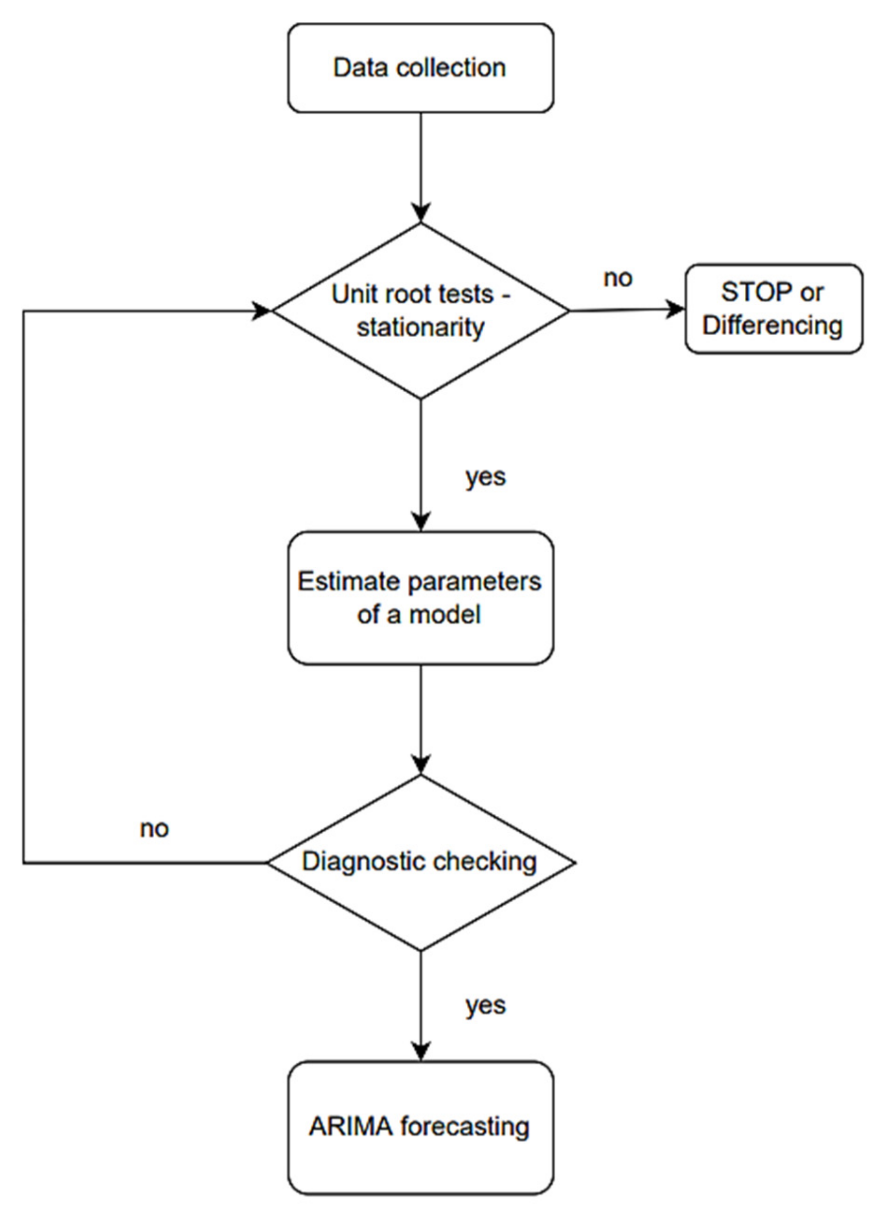
Examining the stationarity of the observed series as a condition for model specifications. If the series is stationary, the procedure continues the step 3, if not–with step 2.

-

Testing the stationarity of the first difference of the observed series.

-

Determining the appropriate ARIMA model based on the ACF and PACF values.

-

Evaluating the ARIMA model.

-

Examining the statistical significance of the model parameters. If they are not significant, the p and q order has to be reduced.

-

Calculating the ACF and PACF residual model (if model is well-estimated, it should be close to zero).

-

Deciding on the best model, according to information criteria and adjusted coefficients of determination. If the model is appropriate, an ARIMA forecast could be obtained. If not, the previous step should be repeated.

Application of the presented methodology was used in the previous research [13,18,27,29].

On the other side, artificial intelligence techniques can be divided into several different approaches, which comprise (but are not limited to) ordinary neural networks; Long Short-Term Memory (LSTM), which is a part of Recurrent Neural Networks (RNNs); and Neural Network Autoregression (NNAR). According to [22], the greatest difference between an ordinary neural network and RNN is that each hidden unit of RNN is not independent—they are not only related to each other but also associated with the sequential input that follows the input of load data at the current moment into the unit of the hidden layer. However, RNNs have proven to possess serious disadvantages, as explained in [22], and those disadvantages have been solved by Long Short-Term Memory (LSTM) [30]. It is a very successful type of neural network, which was introduced by [31]. Nevertheless, even LSTM imposed certain drawbacks, which include training time and accuracy of recognition. Apart from price and/or output forecasting, artificial intelligence methods have been widely used for nowcasting as well (intra-hour forecasts), as explained in [32]. In this particular analysis, Neural Network Autoregression (NNAR) will be compared to ARIMA model, in order to determine which model gives more accurate electricity price forecasts.

NNAR model is defined as a feedforward neural network that includes a linear combination function and an activation function [33,34]. The linear combination function for node j is given as follows:

$$z_j=b_j+{\displaystyle \sum }_{i=1}^n{w}_{ij}{y}_i$$

(2)

where $z_j$ represents the jth hidden layer neuron, n represents the number of input layer neurons, $w_{ij}$ denotes the weights assigned to the connection between the input and the hidden layer, $y_i$ are the observations (covariates or neurons) of the input layer, and the activation function–sigmoid function [34] is given by the following formula:

$$g\left(z\right)=\frac{1}{1-e^{-z}}$$

(3)

By using this process, it is expected that the effects of extreme values will be reduced and that networks will be more resilient to extreme values.

NNAR model enables modeling complex connections between inputs and outputs, while the previously lagged values of the observed time series serve as input for future values forecasting. The Figure 3 presents a previously explained multilayer feed-forward network [33].

Comparison of evaluated models can be done based on several criteria, which include, but are not limited to [28]:

$$\mathrm{Mean} \mathrm{error}:\mathrm{ME}=\frac{1}{g}{{\displaystyle \sum }}_{j=1 }^g\left(x_{m+j}-{\widehat{x}}_{m^{\left(j\right)}}\right)$$

(4)

$$\mathrm{Root} \mathrm{mean} \mathrm{squared} \mathrm{error}:\mathrm{RMSE}=\sqrt{\frac{1}{g}{{\displaystyle \sum }}_{j=1 }^g{\left(x_{m+j}-{\widehat{x}}_{m^{\left(j\right)}}\right)}^2 }$$

(5)

$$\mathrm{Mean} \mathrm{absolute} \mathrm{error}:\mathrm{MAE}=\frac{1}{g}{{\displaystyle \sum }}_{j=1 }^g\left|x_{m+j}-{\widehat{x}}_{m^{\left(j\right)}}\right|$$

(6)

$$\mathrm{Mean} \mathrm{percentage} \mathrm{error}:\mathrm{MPE}=\frac{100}{g}{{\displaystyle \sum }}_{j=1}^g\frac{x_{m+j}-{\widehat{x}}_{m^{\left(j\right)}}}{x_{m+j}}=\frac{100}{g} {{\displaystyle \sum }}_{j=1}^{g}1-\frac{{\widehat{x}}_{m^{\left(j\right)}}}{x_{m+j}}$$

(7)

$$\mathrm{Mean} \mathrm{absolute} \mathrm{percentage} \mathrm{error}: \mathrm{MAPE}=\frac{100}{g}{{\displaystyle \sum }}_{j=1}^g\left|\frac{x_{m+j}-{\widehat{x}}_{m^{\left(j\right)}}}{x_{m+j}}\right|$$

(8)

$$\mathrm{Theil}\prime \mathrm{s} \mathrm{U} \mathrm{statistics}: \mathrm{U}=\sqrt{\frac{{{\displaystyle \sum }}_{j=1}^{g-1}{\left(\frac{{\widehat{X}}_{j+1}-X_{j+1}{}_{ }}{X_j}\right)}^2}{{{\displaystyle \sum }}_{j=1}^{g-1}{\left(\frac{X_{j+1}-X_j{}_{ }}{X_j}\right)}^2}}$$

(9)

where g is the number of data points, $x_{m+j}$ is the actual value, ${\widehat{x}}_{m^{\left(j\right)}}$ is the predicted value, and $x_{m+j}-{\widehat{x}}_{m^{\left(j\right)}}$ is the forecast error. Regarding the Theil’s U statistic, $X_j$ is the actual value of a point for a given time period j, and ${\widehat{X}}_j$ is the forecasted value. Smaller values of forecast-accuracy statistics correspond to a better forecast model.

After the electricity price forecast has been conducted (prices have been forecasted on a daily level for the following period: 25 May 2022–31 December 2022), several methods for economic viability analysis will be implemented. These include net present value (NPV), internal rate of return (IRR), payback period (PBP), and the levelized cost of energy (LCOE).

NPV, or the difference between the present value of future cash flows expected during the lifetime of the investment and the initial investment at year zero, can be calculated as follows [35]:

$$\mathrm{NPV}={\displaystyle \sum }_{t=1}^n\frac{{CF}_t}{{\left(1+i\right)}^n}{-I}_0$$

(10)

where $C{F}_t$ is the cash flow in year $t$, $n$ is the lifetime of the investment, $i$ is the discount rate, and $I_0$ is an initial investment at year zero.

IRR, by definition [36], is a discount rate that sets NPV equal to zero. Mathematically written, NPV calculated with IRR as a discount rate would be the following:

$$\mathrm{NPV}={{\displaystyle \sum }}_{t=1}^n\frac{C{F}_t}{{\left(1+\mathrm{IRR}\right)}^n}-I_0=0$$

(11)

IRR helps us determine which projects are more viable (the lower the IRR is, the higher the NPV), as it can be seen as the highest discount rate acceptable for a project. Any project with a discount rate higher than IRR has a negative NPV, therefore, it is considered not viable.

PBP is the time needed for the cash flows from the project to surpass the amount of the initial investment needed for the project. PBP can be also defined as the year in which NPV becomes positive. The main approaches to PBP are simple and discounted, though only the discounted approach has been used widely (due to the fact that the simple approach does not account for the time value of money). Discounted PBP is calculated as follows [37]:

$$\mathrm{DPP}=\frac{\left(\frac{1}{1-\frac{I_0\times i}{CF}}\right)}{\ln \left(1+i\right)}$$

(12)

where $I_0$ is the initial investment, $i$ is the rate, and CF is the periodic cash flow.

LCOE is the total cost for each MWh or kWh including capital cost, operating cost, and maintenance (O&M cost), based on capacity and useful life [35]. LCOE can be calculated by dividing annual expenditures (investment and O&M) with annual electricity generation [38]. Mathematically, LCOE would be calculated as follows:

$$\mathrm{LCOE}=\frac{{{\displaystyle \sum }}_{t=1}^n\frac{I_t+M_t}{{\left(1+i\right)}^n}}{{{\displaystyle \sum }}_{t=1}^n\frac{E_t}{{\left(1+i\right)}^n}}$$

(13)

where $I_t$ is the investment expenditures, $M_t$ is the operations and maintenance expenditures, $E_t$ is the electricity generation$, i$ is the discount rate, $n$ is the system’s lifetime, and $t$ is the year.

Sensitivity analysis will be conducted by changing the electricity price, balancing cost, annual production, and the weighted average cost of capital (WACC). Changes in these variables will be reflected by adjusting all four parameters accordingly–NPV, IRR, PBP, and LCOE.

3. Case Study

In order to conduct a proper economic analysis of the proposed project, internal data from the investor have been obtained. The

Table 1. Capital expenditures for the 5 MW solar power plant.

CAPEX Analysis
Category	Amount
Land plot acquisition	EUR 250,000
Grid connection fee	EUR 190,000
Main project design	EUR 50,000
Groundworks	EUR 210,000
Concrete works	EUR 170,000
Metal substructure with installation	EUR 375,000
Solar modules and inverters with installation	EUR 1,650,000
Substation with construction works	EUR 350,000
Electric and other cables	EUR 280,000
Supervision works	EUR 60,000
Other construction works	EUR 180,000
Overheads (10%)	EUR 376,500
Total	EUR 4,141,500
Total per kW	EUR 828.30

Source: Main project design–PV Kuči [39].

present a detailed breakdown of the expected capital expenditures (CAPEX) for this project, based on obtained offers and signed engineering, procurement, and construction (EPC) contracts. Prices below are displayed without VAT, since the VAT will be reimbursed to the investor. Additionally, during the engineering phase, detailed predictions of the solar power plant production have been established as well as the anticipated operating expenses (OPEX) during the facility-production phase.

Based on different software simulations of the facility production, the results have been obtained. The expected annual production of the PV power plant in Podgorica is 6841 MWh. A brief extract from one of the simulations conducted is shown in the Figure 4.

The empirical data in this paper contain hourly electricity price data. They were downloaded from the Hungarian Power Exchange [40]. Hourly data from 1 January 2020 up to 25 May 2021 were used to forecast electricity prices using the ARIMA and NNAR models. The total number of days observed was 485. In order to pair the daily production of the solar power plant with the prices, we took the average price of the obtained hourly data from 7 am to 7 pm. Therefore, the number of observations in the table represents the number of instances in the analysis, which equals the number of days. Descriptive statistics of the sample are shown in

Table 2. Descriptive statistics of analyzed prices.

Series	Values
Observations	485
Mean	139.9281
Median	113.2758
Maximum	544.7283
Minimum	14.89583
Std. Dev.	85.20709
Skewness	0.951737
Kurtosis	3.950774
Jarque–Bera	91.48687
Probability	0

. The average electricity price in the data sample is 139.92 EUR/MWh, while the standard deviation equals 85.20 EUR/MWh.

Typically, a dataset is split into training and test sets in an 80:20 proportion. However, the immediate effects of war aggression in Ukraine would severely disrupt price forecasts. Therefore, we have chosen a different proportion of training and test data. The training data include electricity prices for the period 1 January 2021–1 May 2022, while the test data include electricity prices from 1 May 2022 up to 25 May 2022.

4. Results

As previously mentioned, the methods that were used in price forecasting are ARIMA and NNAR.

The parameters of the ARIMA model are shown in

Table 3. Estimated ARIMA model.

Variable	Coefficient	Std. Error	t-Statistic	Prob.
C	0.381232	0.173292	2.199938	0.0283
AR (1)	0.771313	0.036749	20.98848	0.0000
MA (1)	−0.972690	0.013996	−69.49627	0.0000

, and they were estimated using the lowest values of AIC information criteria.

The NNAR model was estimated in RStudio software package, using the automatic process for estimation of NNAR via the nnetar function. Parameters were estimated, as shown in

Table 4. Estimated NNAR model.

Model
NNETAR Series: p1 NNAR (22,1,12) [365] Call: nnetar (y = p1, lambda = “0”) Average of 20 networks, each of which is a 23-12-1 network with 301 weights options were–linear output units
${\sigma }^2$ estimated as 0.0002105

.

In order to compare the forecasting accuracy of both models selected for the analysis, ME, RMSE, MAE, MPE, and Theil’s U parameters have been calculated for the testing period. This part of the analysis aims to examine the differences between the predicted and actual values. In

Table 5. Criteria for evaluation of forecasts.

Model
Criteria	ARIMA	NNAR
ME	−20.26215	3.16550823
RMSE	36.89402	34.2124869
MAE	28.46972	28.2489473
MPE	−12.20065	2.380968496
MAPE	15.54559	14.3177964
Theil’s U	1.0893	1.006192

, it can be seen that NNAR proved to be a more accurate forecasting tool, as values for RMSE (34.2124869 < 36.89402), MAE (28.2489473 < 28.46972), MAPE (14.3177964 < 15.54559), and Theil’s U (1.006192 < 1.0893) tend to be lower for NNAR than for ARIMA. In general, models with the lowest values of parameters are considered more accurate in forecasting. Consequently, NNAR was evaluated as a better forecasting tool in this particular analysis.

Figure 5 shows forecasts done by ARIMA (red), NNAR (green), and real prices (blue). The graphical presentation shows more clearly the differences between ARIMA and NNAR’s abilities to predict future electricity prices on the market. The green line on the graph authentically follows the real price fluctuation. Therefore, the graph justifies that the NNAR model forecast imitates real changes better than the ARIMA model does.

The succeeding element of the analysis implies forecasting electricity prices for the time period, based on the outcomes of the previous steps. Due to the fact that NNAR showed better results in the testing phase, we have completed this part of the analysis by using it. The forecast performed using the NNAR model is given in Figure 6 and contains the whole dataset with the prices obtained. The graph of the pre-forecast prices shows two peaks–the first one due to the lack of gas and electricity for heating (winter months), while the second one happened due to the start of the war in Ukraine. The forecast on the graph shows a stable price-moving trend for the second half of 2022, up until the beginning of 2023, with the range being mostly $\pm 20$ EUR from the average value. Estimated NNAR model parameters are given in the

Table 6. Estimated NNAR model.

Model

NNAR (27,1,14) [365] Call: nnetar (y = p, lambda = “0”) Average of 20 networks, each of which is a 28-114-1 network with 421 weights options were–linear output units

${\sigma }^2$ estimated as 0.0001958

.

The average of forecasted daily electricity prices using NNAR was derivate at 155.40 EUR/MWh. This value was implemented in the second part of the analysis, where a financial evaluation of this project was performed. Namely, taking into consideration the current energy crisis and tendency to transform this industry towards a greener one, as well as political turmoil associated with the war in Ukraine, the assumption is made that this price level will remain for the mid-term.

The results obtained from the electricity prices econometric analysis, coupled with relevant information regarding CAPEX and OPEX of this photovoltaic power plant form the complete input data for the project financial analysis. In order to calculate electricity price on the production site of this facility, a calculation of costs associated with delivering electricity to the location defined by electricity market rules was conducted. Those costs involved fees to the national grid operator [41,42,43], well as inter-connection costs, cost of balancing the production of the plant, and fees for the electricity trading company who will in this case manage grid capacity booking, balancing activities, and access to the exact electricity exchange. The trader will conduct stated business activities as a service in the name of the owner, without taking any risks associated with the ownership of electricity. Overall risk remains at the side of the solar plant owner, alongside potential gains. On-site electricity price calculation is displayed in

Table 7. On-site electricity price calculation.

Electricity Price Calculation
Category	Amount
Average electricity price on HUPX	EUR 155.40
Grid operator fee	EUR −13.00
Balancing cost (% of the price on the market)	EUR −17.09
Trader’s fee (% of the price on the market)	EUR −4.66
Electricity price	EUR 120.64
Expected annual production (/MWh)	6841
Annual income	EUR 825,325.60

.

Based on the expected market price for this kind of service and assumed balancing cost relied on the historic trend from the experienced trading company, on-site electricity price has been calculated. Hence, the electricity price was derivate at 120.64 EUR/MWh, and it is significantly higher than the prices that could be obtained through a standard PPA [44] mid-term contract for this region.

As previously highlighted, the initial assumption of this paper is to extend the obtained average electricity price for the following years and derivate the financial analysis accordingly. Taking this into consideration, for the first five years of production, the stated electricity price level has been taken. The remaining exploitation period is linked with a fixed price, in line with the price that could be obtained on the market for long-term PPA contracts. Financial analysis has included the discount rate taken over from Damodaran’s database [45], for the green and renewable energy for emerging markets (5.81%). Four criteria for the evaluation of the financial soundness of this project have been calculated and are shown in

Table 8. Financial parameters of the PV plant.

Parameter	Unit	Value
NPV	€	2,780,054.33
LCOE	€/MWh	58.89
IRR	%	12.93
PBP	Years	7.1

.

As seen in the table, the net present value of this project is almost EUR 2.8 million, while the payback period of the investment is determined at 7.1 years, with one year intended for the construction phase. The internal rate of return is adequate and acceptable, at the value of 12.93%. At the same time, the levelized cost of electricity, of 58.89 EUR/MWh, is relatively high.

Since the business strategy developed through this analysis is a perilous one, conducting sensitivity tests as part of it is of high importance. Sensitivity analysis contained an observation of the most uncertain elements and their effect on previously interpreted financial parameters (NPV, LCOE, IRR, and PBP). Selected variables for the sensitivity analysis are electricity price, due to its fluctuation on the exchange market, balancing cost, annual electricity production of the solar plant, and change in the weighted average cost of capital. Namely, the WACC for this industry for Europe, instead of the WACC for emerging markets, has been considered. Additionally, financial analysis of the same project, with fixed PPA instead of a riskier market price, has been shown in order to draw appropriate conclusions. Obtained values are displayed in

Table 9. Sensitivity analysis of the PV plant financial values.

Variables	Electricity Price −20%	Electricity Price +20%	Fixed PPA	Balancing Cost +30%	Balancing Cost −10%	Annual Production −10%	Annual Production +5%	WACC for Europe Instead of Emerging Markets
NPV	−24.28%	24.28%	−36.92%	−4.66%	1.56%	−25.81%	12.91%	3.85%
LCOE	−1.72%	1.71%	−2.60%	−0.33%	0.11%	9.09%	−3.89%	−1.19%
IRR	−17.00%	19.90%	−24.79%	−3.48%	1.19%	−13.94%	6.95%	0.00%
PBP	26.76%	−27.46%	40.85%	5.63%	−1.41%	14.08%	−2.82%	−1.41%

.

Net present value, internal rate of return, and payback period of this project have been most affected by changes in electricity price, including the fixed PPA alternative and discrepancies in the exact electricity production from the expected level. Logically, when NPV and IRR decrease, the payback period increases, and vice versa. On the other hand, the LCOE of this project shows greater consistency, and it is less affected by potential changes. In general, that is the effect of its nature, since it does not involve a price element in the calculation. These results indicate LCOE is mostly affected by changes in annual production. Overall, the results of this analysis suggest this project has its financial stability and quality to be undertaken swiftly, but without neglecting its potential financial risks and downsides.

5. Discussion and Conclusions

This study investigates the financial viability of a 5 MW solar power plant in Montenegro, which is commencing production in Q4 2022. The interesting feature of this analysis relates to a different business model, which includes entering the market directly. The aim is to assess gains from this strategic approach to the market, while taking into consideration the increased immanent risks. Econometric analysis of electricity prices on the exchange market has been conducted via two different tools. NNAR showed significantly better results in predicting electricity prices and was used to forecast prices for the following months. The obtained average price is 155.4 EUR/MWh, and it could probably be a higher value if the analysis did not cover the first half of 2021, when a spike in prices was not visible yet.

The calculated financial parameters of this project are satisfactory and in favor of project implementation, via the business model displayed in this paper. If assumptions made in this analysis are achieved in the mid-term, the payback period of this project will be 7.1 years. The LCOE of this project is obtained at the value of 58.89 EUR/MWh, which is higher than assessed by the International Renewable Energy Agency [4], and it reflects mostly inflation pressure and shortage of raw materials through its capital expenditures during 2022 as well as the smaller scale of the project. Sensitivity analysis showed relative changes in the financial parameters for this project, when the most uncertain input elements alternate. The conclusion may be drawn that changes in electricity prices on the market significantly influence the profitability of this project; however, the values are still notably higher than in the case of a fixed PPA contract for the investor, when PBP would be 40% longer.

The uncertainty associated with the current geopolitical situation and a shift toward greener energy sources has induced higher prices in the markets, with expectations to prevail at a similar level in the future. Hence, the business environment will remain in favor of a riskier strategy—entering the market directly, as displayed in this paper, or advance power-purchase arrangements splitting risks and gains between producers and traders in some proportion. The described business models would improve the relatively modest returns and accelerate changes in the energy sector towards renewable sources. Speeding up transformation processes must be at the top of the policy and business priorities, to prevent future deterioration of the environment as well as achieve very much-needed energy independence.

The main limitation of this paper is related to the way future electricity prices are estimated, due to the extremely high uncertainty in the market. Additional limitation refers to a high day-to-day production volatility and, therefore, an inability to pair hourly electricity prices with the corresponding production. However, economic performance and technical development of technological projects are always affected by uncertainties associated with market fluctuations, which require careful consideration and appropriate risk analysis [14].

References

1. Manoj Kumar, N.; Sudhakar, K.; Samykano, M. Techno-Economic Analysis of 1 MWp Grid Connected Solar PV Plant in Malaysia. Int. J. Ambient Energy 2019, 40, 434–443. [Google Scholar] [CrossRef]
2. Althuwaini, Y.E.Y.Y.E.; Philbin, S.P. Techno-Economic Analysis of Solar Power Plants in Kuwait: Modelling the Performance of PV and CSP Systems. Int. J. Renew. Energy Res. 2021, 11, 2009–2024. [Google Scholar] [CrossRef]
3. Saleh, A.; Faridun, M.; Tajuddin, N.; Eddine, T.; Zidane, K.; Su, C.; Jawad, A.; Alrubaie, K.; Alwazzan, M.J. Techno-Economic and Environmental Evaluation of PV/Diesel/Battery Hybrid Energy System Using Improved Dispatch Strategy. Energy Rep. 2022, 8, 6794–6814. [Google Scholar] [CrossRef]
4. IEA. Electricity Market Report; IEA: Paris, France, 2022. [Google Scholar]
5. Agga, A.; Abbou, A.; Labbadi, M.; El Houm, Y. Short-Term Self Consumption PV Plant Power Production Forecasts Based on Hybrid CNN-LSTM, ConvLSTM Models. Renew. Energy 2021, 177, 101–112. [Google Scholar] [CrossRef]
6. Gürtürk, M. Economic Feasibility of Solar Power Plants Based on PV Module with Levelized Cost Analysis. Energy 2019, 171, 866–878. [Google Scholar] [CrossRef]
7. Solouki, A.; Jaffer, S.A.; Chaouki, J. Process Development and Techno-Economic Analysis of Microwave-Assisted Demetallization and Desulfurization of Crude Petroleum Oil. Energy Rep. 2022, 8, 4373–4385. [Google Scholar] [CrossRef]
8. Le, P.T.; Nguyen, V.D.; Le, P.L. Techno-Economic Analysis of Solar Power Plant Project in Binh Thuan, Vietnam. In Proceedings of the 2018 4th International Conference on Green Technology and Sustainable Development (GTSD), Ho Chi Minh City, Vietnam, 23–24 November 2018; pp. 82–85. [Google Scholar] [CrossRef]
9. Elnajjar, H.M.; Shehata, A.S.; Elbatran, A.H.A.; Shehadeh, M.F. Experimental and Techno-Economic Feasibility Analysis of Renewable Energy Technologies for Jabel Ali Port in UAE. Energy Rep. 2021, 7, 116–136. [Google Scholar] [CrossRef]
10. Cui, T.; Wang, C.; Nie, P.Y. Economic Analysis of Marsh Gas Development in Countryside of China: A Case Study of Gongcheng County in Guangxi Province. Energy Rep. 2019, 5, 462–466. [Google Scholar] [CrossRef]
11. Tcvetkov, P.; Cherepovitsyn, A.; Makhovikov, A. Economic Assessment of Heat and Power Generation from Small-Scale Liquefied Natural Gas in Russia. Energy Rep. 2020, 6, 391–402. [Google Scholar] [CrossRef]
12. Zou, X.; Qiu, R.; Yuan, M.; Liao, Q.; Yan, Y.; Liang, Y.; Zhang, H. Sustainable Offshore Oil and Gas Fields Development: Techno-Economic Feasibility Analysis of Wind–Hydrogen–Natural Gas Nexus. Energy Rep. 2021, 7, 4470–4482. [Google Scholar] [CrossRef]
13. Contreras, J.; Espínola, R.; Nogales, F.J.; Conejo, A.J. ARIMA Models to Predict Next-Day Electricity Prices. IEEE Trans. Power Syst. 2003, 18, 1014–1020. [Google Scholar] [CrossRef]
14. Wu, L.; Shahidehpour, M. A Hybrid Model for Day-Ahead Price Forecasting. IEEE Trans. Power Syst. 2010, 25, 1519–1530. [Google Scholar] [CrossRef]
15. Colantoni, A.; Villarini, M.; Monarca, D.; Carlini, M.; Mosconi, E.M.; Bocci, E.; Rajabi Hamedani, S. Economic Analysis and Risk Assessment of Biomass Gasification CHP Systems of Different Sizes through Monte Carlo Simulation. Energy Rep. 2021, 7, 1954–1961. [Google Scholar] [CrossRef]
16. Anbazhagan, S.; Kumarappan, N. Day-Ahead Deregulated Electricity Market Price Forecasting Using Neural Network Input Featured by DCT. Energy Convers. Manag. 2014, 78, 711–719. [Google Scholar] [CrossRef]
17. Zhou, X.; Yang, J.; Wang, F.; Xiao, B. Economic Analysis of Power Generation from Floating Solar Chimney Power Plant. Renew. Sustain. Energy Rev. 2009, 13, 736–749. [Google Scholar] [CrossRef]
18. Gao, G.; Lo, K.; Fan, F.; Gao, G.; Lo, K.; Fan, F. Comparison of ARIMA and ANN Models Used in Electricity Price Forecasting for Power Market. Energy Power Eng. 2017, 9, 120–126. [Google Scholar] [CrossRef]
19. Shafie-Khah, M.; Moghaddam, M.P.; Sheikh-El-Eslami, M.K. Price Forecasting of Day-Ahead Electricity Markets Using a Hybrid Forecast Method. Energy Convers. Manag. 2011, 52, 2165–2169. [Google Scholar] [CrossRef]
20. Box, G.E.P.; Jenkins, G.M.; Reinsel, G.C.; Ljung, G.M. Time Series Analysis: Forecasting and Control, 5th ed.; Wiley: Hoboken, NJ, USA, 2015; ISBN 978-1-118-67502-1. [Google Scholar]
21. Lo, K.L.; Wu, Y.K. Risk Assessment Due to Local Demand Forecast Uncertainty in the Competitive Supply Industry. IEE Proc. Gener. Transm. Distrib. 2003, 150, 573–582. [Google Scholar] [CrossRef]
22. Chen, Z.; Zhang, D.; Jiang, H.; Wang, L.; Chen, Y.; Xiao, Y.; Liu, J.; Zhang, Y.; Li, M. Load Forecasting Based on LSTM Neural Network and Applicable to Loads of “Replacement of Coal with Electricity”. J. Electr. Eng. Technol. 2021, 16, 2333–2342. [Google Scholar] [CrossRef]
23. Reza, A.; Debnath, T. An Approach to Make Comparison of ARIMA and NNAR Models For Forecasting Price of Commodities. 2020. Available online: https://www.researchgate.net/publication/342563043_An_Approach_to_Make_Comparison_of_ARIMA_and_NNAR_Models_For_Forecasting_Price_of_Commodities (accessed on 1 June 2022).
24. Alfares, H.K.; Nazeeruddin, M. Electric Load Forecasting: Literature Survey and Classi®cation of Methods. Int. J. Syst. Sci. 2002, 33, 23–34. [Google Scholar] [CrossRef]
25. Aggarwal, S.K.; Saini, L.M.; Kumar, A. Electricity Price Forecasting in Deregulated Markets: A Review and Evaluation. Int. J. Electr. Power Energy Syst. 2009, 31, 13–22. [Google Scholar] [CrossRef]
26. Lago, J.; Marcjasz, G.; De Schutter, B.; Weron, R. Forecasting Day-Ahead Electricity Prices: A Review of State-of-the-Art Algorithms, Best Practices and an Open-Access Benchmark. Appl. Energy 2021, 293, 116983. [Google Scholar] [CrossRef]
27. Jakaša, T.; Andročec, I.; Sprčić, P. Electricity Price Forecasting ARIMA Model Approach. In Proceedings of the 2011 8th International Conference on the European Energy Market (EEM), Zagreb, Croatia, 25–27 May 2011; pp. 222–225. [Google Scholar] [CrossRef]
28. Box, G.E.P.G.M.J. Time Series Analysis, Control and Forecasting; Holden Day: San Francisco, CA, USA, 1976. [Google Scholar]
29. Karadžić, V.; Pejovic, B. Inflation Forecasting in the Western Balkans and EU: A Comparison of Holt-Winters, ARIMA and NNAR Models. Amfiteatru Econ. 2021, 23, 517. [Google Scholar] [CrossRef]
30. Nespoli, A.; Ogliari, E.; Pretto, S.; Gavazzeni, M.; Vigani, S.; Paccanelli, F. Electrical Load Forecast by Means of LSTM: The Impact of Data Quality. Forecast 2021, 3, 91–101. [Google Scholar] [CrossRef]
31. Hochreiter, S.; Schmidhuber, J. Long Short-Term Memory. Neural Comput. 1997, 9, 1735–1780. [Google Scholar] [CrossRef]
32. Sala, S.; Amendola, A.; Leva, S.; Mussetta, M.; Niccolai, A.; Ogliari, E. Comparison of Data-Driven Techniques for Nowcasting Applied to an Industrial-Scale Photovoltaic Plant. Energies 2019, 12, 4520. [Google Scholar] [CrossRef]
33. Hyndman, R.J.; Athanasopoulos, G. Forecasting: Principles and Practice. Princ. Optim. Des. 2018, 504, 46–48. [Google Scholar]
34. Da Silva, F.L.C.; da Costa, K.; Rodrigues, P.C.; Salas, R.; López-Gonzales, J.L. Statistical and Artificial Neural Networks Models for Electricity Consumption Forecasting in the Brazilian Industrial Sector. Energies 2022, 15, 588. [Google Scholar] [CrossRef]
35. Han, J.; Moraga, C. The Influence of the Sigmoid Function Parameters on the Speed of Backpropagation Learning. Lect. Notes Comput. Sci. 1995, 930, 195–201. [Google Scholar] [CrossRef]
36. Dubey, R.; Joshi, D.; Bansal, R.C. Optimization of Solar Photovoltaic Plant and Economic Analysis. Electr. Power Compon. Syst. 2016, 44, 2025–2035. [Google Scholar] [CrossRef]
37. Zala, J.N.; Jain, P. Design and Optimization of a Biogas-Solar-Wind Hybrid System for Decentralized Energy Generation for Rural India. Int. Res. J. Eng. Technol. 2017, 37, 1–8. [Google Scholar]
38. Al-Khori, K.; Bicer, Y.; Koç, M. Comparative Techno-Economic Assessment of Integrated PV-SOFC and PV-Battery Hybrid System for Natural Gas Processing Plants. Energy 2021, 222, 119923. [Google Scholar] [CrossRef]
39. Sistem-MNE. Main Project Design-PV Kuči; Sistem-MNE: Podgorica, Montenegro, 2022. [Google Scholar]
40. HUPX. Historic data. Available online: https://hupx.hu/en/market-data/dam/historical-data (accessed on 25 May 2022).
41. Cedis Doo. Metodologija za odredjivanje cijena. Available online: http://cedis.me/regulativa/ (accessed on 25 May 2022).
42. CGES. Metodologija za odredjivanje cijena prenosnih kapaciteta. Available online: https://www.cges.me/regulativa/interna-akta-cges-a (accessed on 25 May 2022).
43. SEE CAO. Dnevni rezulatati aukcija. Available online: https://www.seecao.com/daily-results (accessed on 25 May 2022).
44. Pexapark. PPA transaction database. Available online: https://pexapark.com/ppa-checklist/ (accessed on 25 May 2022).
45. Damodaran, A. Useful Data Sets. Available online: https://pages.stern.nyu.edu/~adamodar/New_Home_Page/datacurrent.html (accessed on 20 June 2022).
Figure 1. Electricity price forecasting models [24].
Energies 15 06219 g001
Figure 2. Flowchart of ARIMA modeling and forecasting [28].
Energies 15 06219 g002
Figure 3. A diagrammatic representation of the NNAR (p, P, k) model.
Energies 15 06219 g003
Figure 4. Expected annual production of the solar power plant. Source: Main project design–PV Kuči [39].
Energies 15 06219 g004
Figure 5. Price forecast comparison–ARIMA, NNAR, and real prices.
Energies 15 06219 g005
Figure 6. Price forecast using NNAR model.
Energies 15 06219 g006