


Extraction of Urban Quality of Life Indicators Using Remote Sensing and Machine Learning: The Case of Al Ain City, United Arab Emirates (UAE)


Abstract
1. Introduction
2. Material and Methods
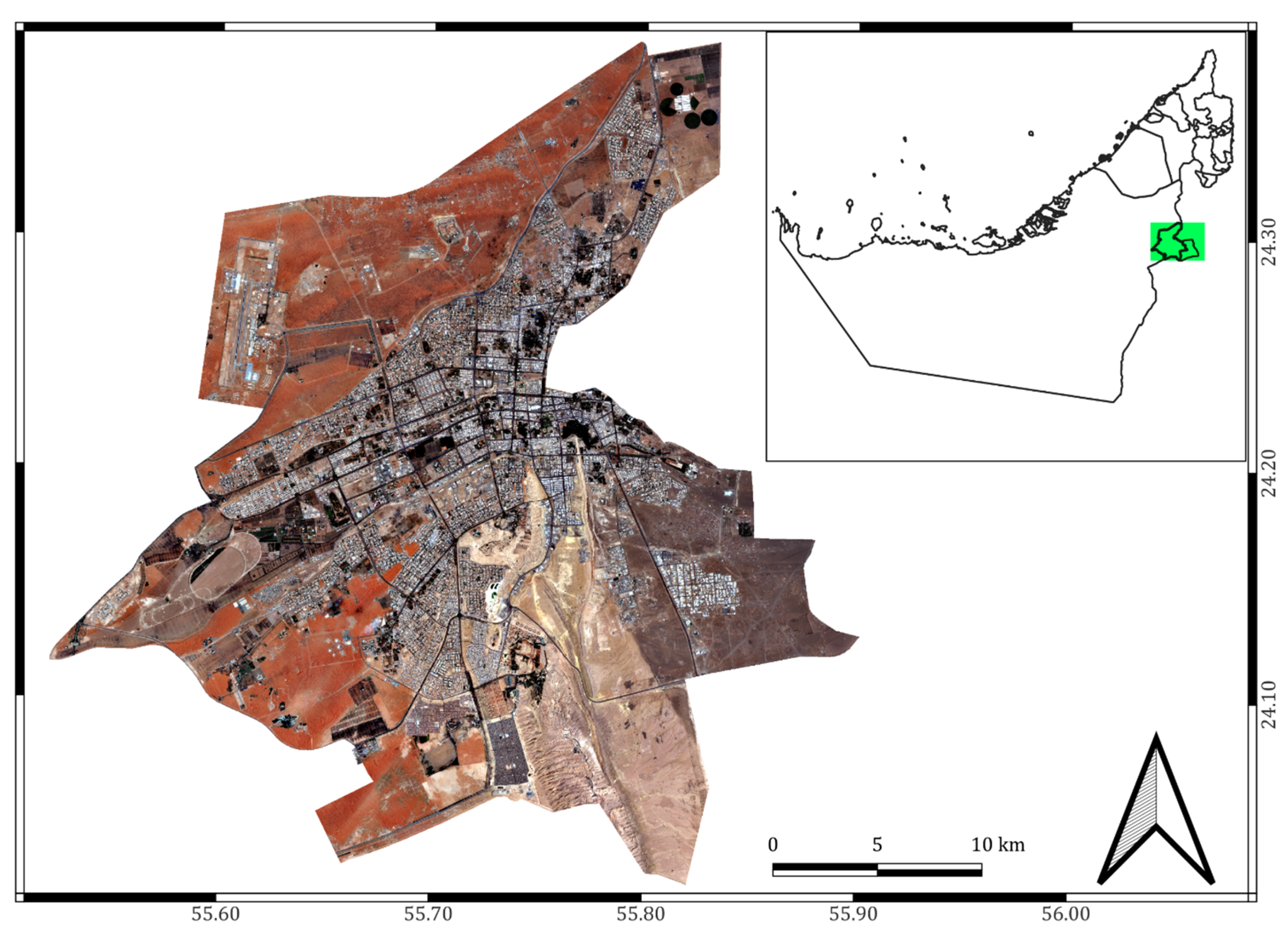
2.1. Study Area
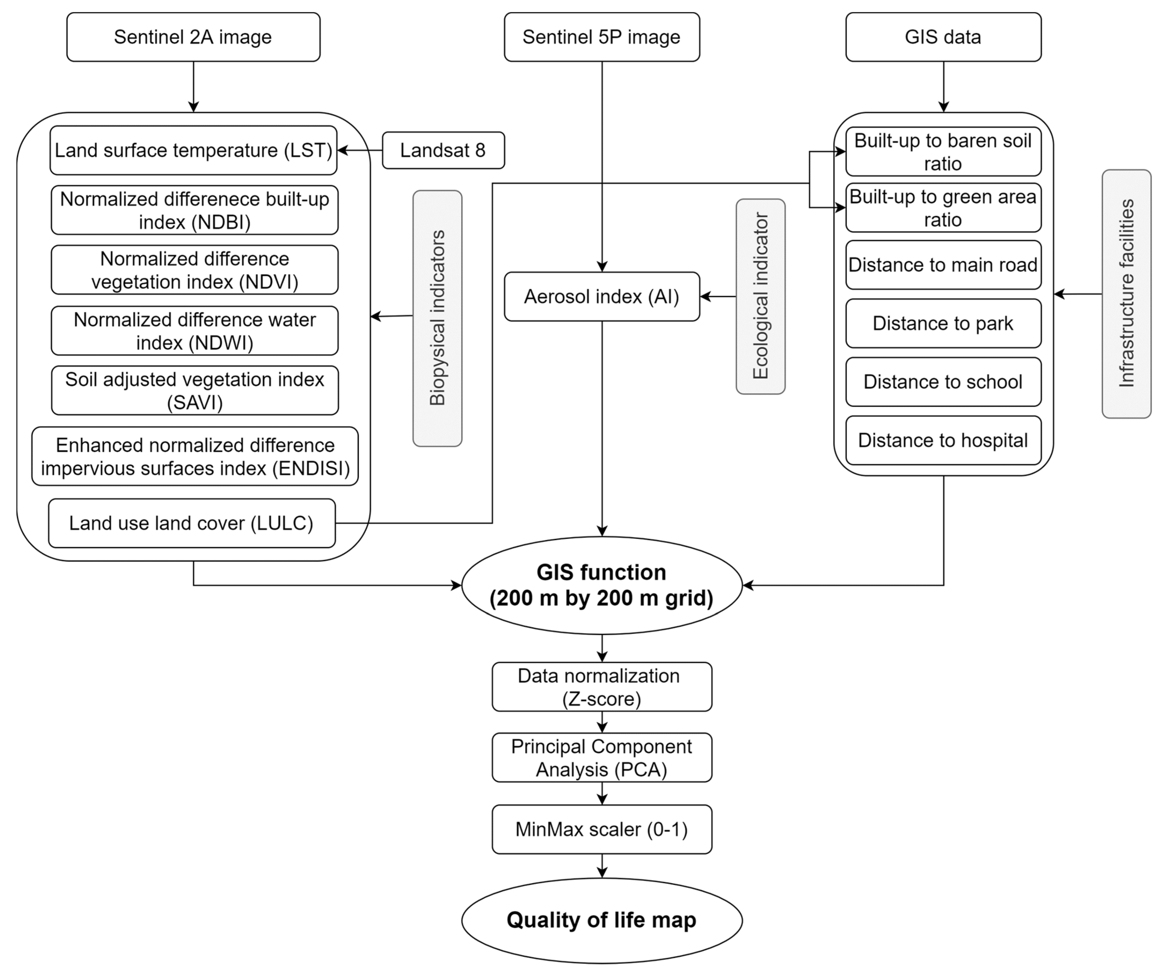
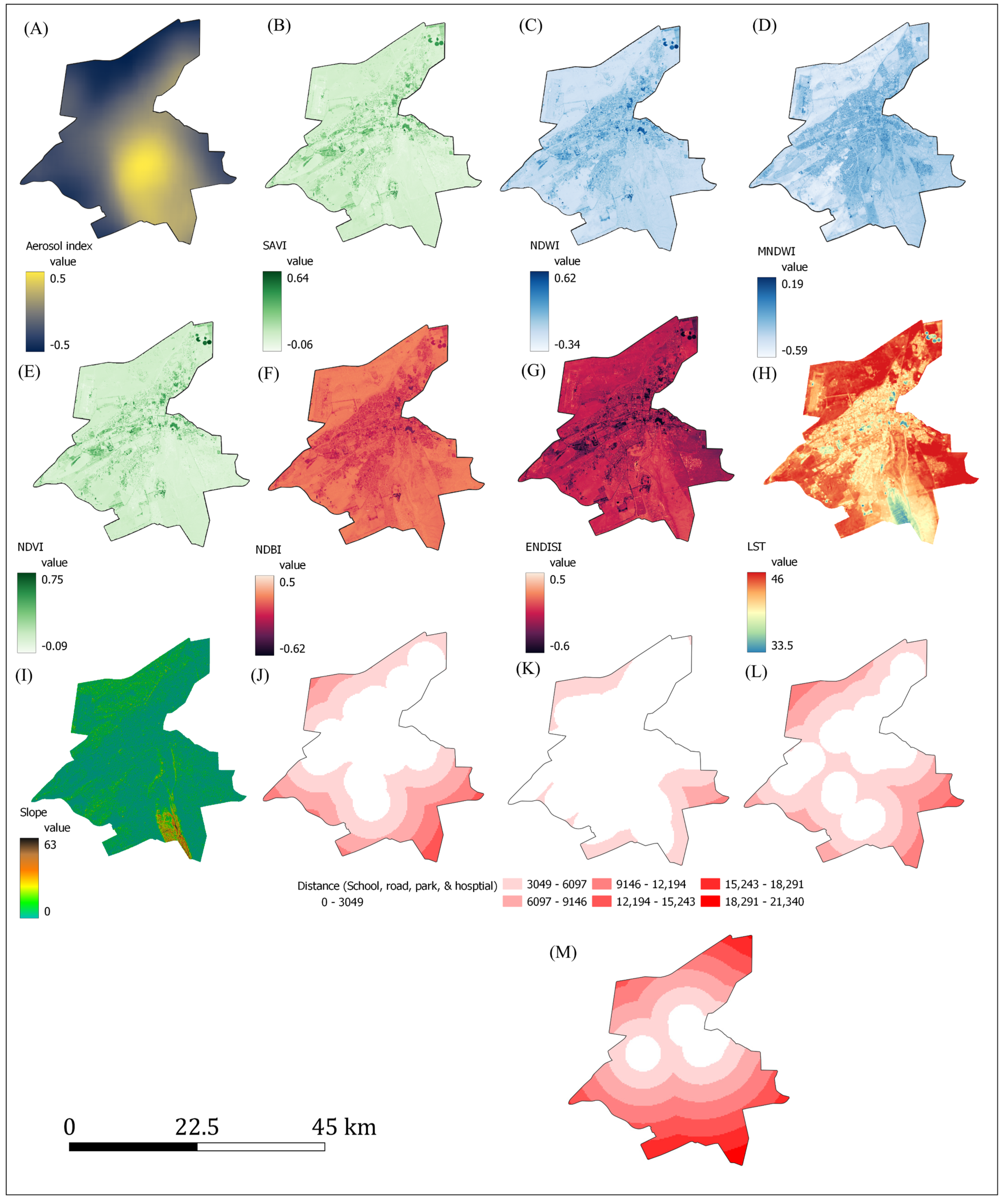
2.2. Datasets and Extraction of Environmental Variables
2.3. Land Use Land Cover Classification Using a Machine Learning Algorithm
2.4. Integration of Environmental and Infrastructure Facility Data
2.5. Urban Quality of Life Index and Validation Procedure
3. Results
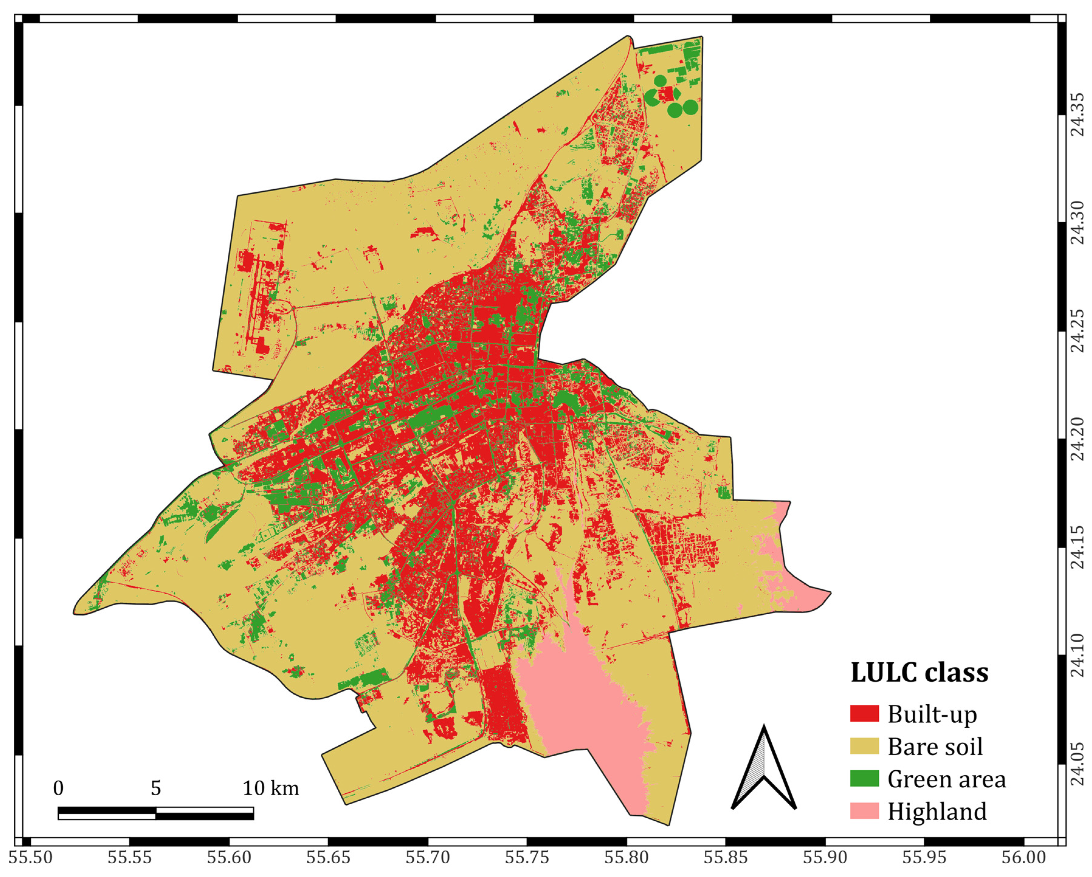
3.1. Land Use Land Cover Classification
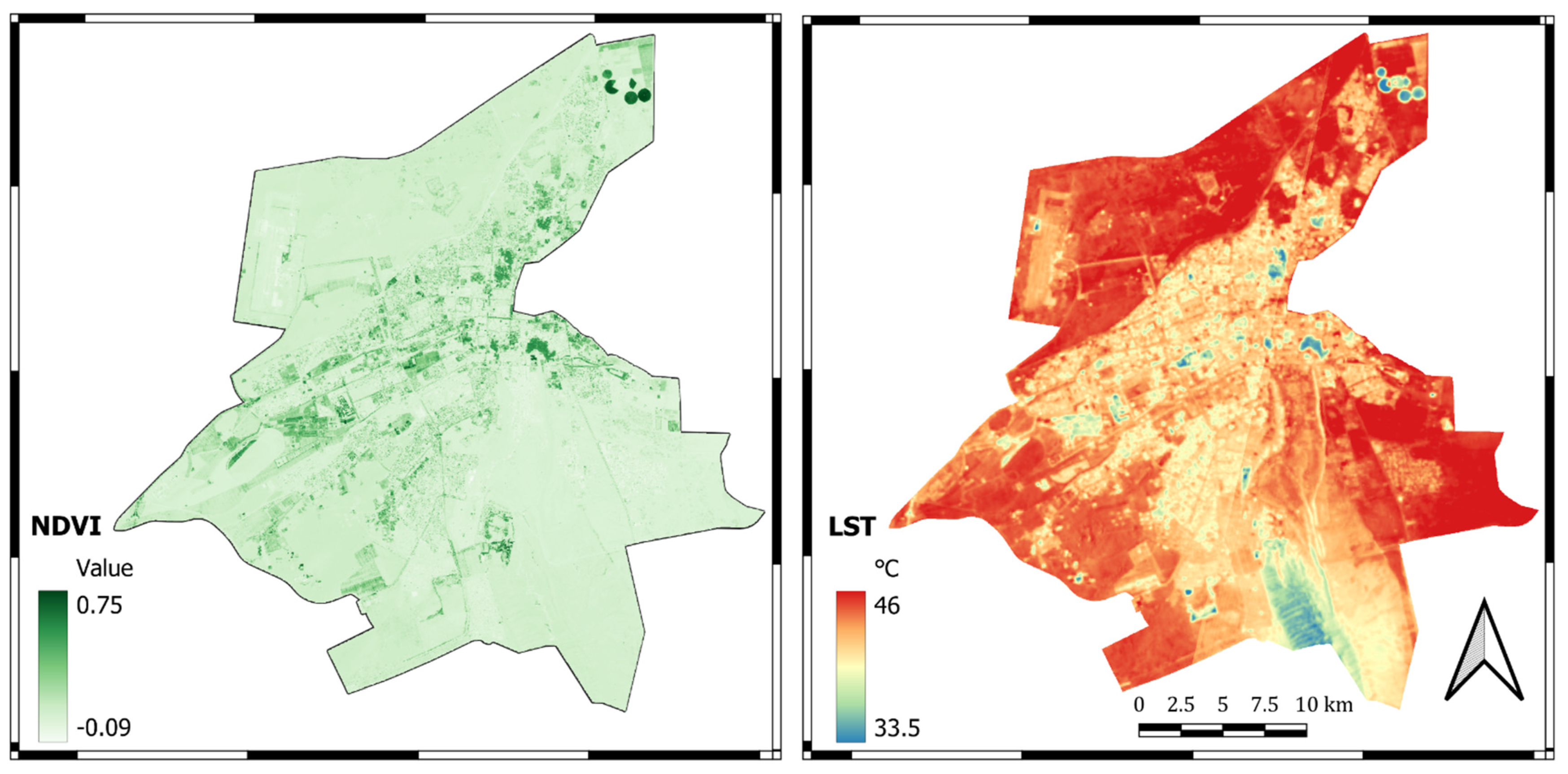
3.2. Statistical Analysis
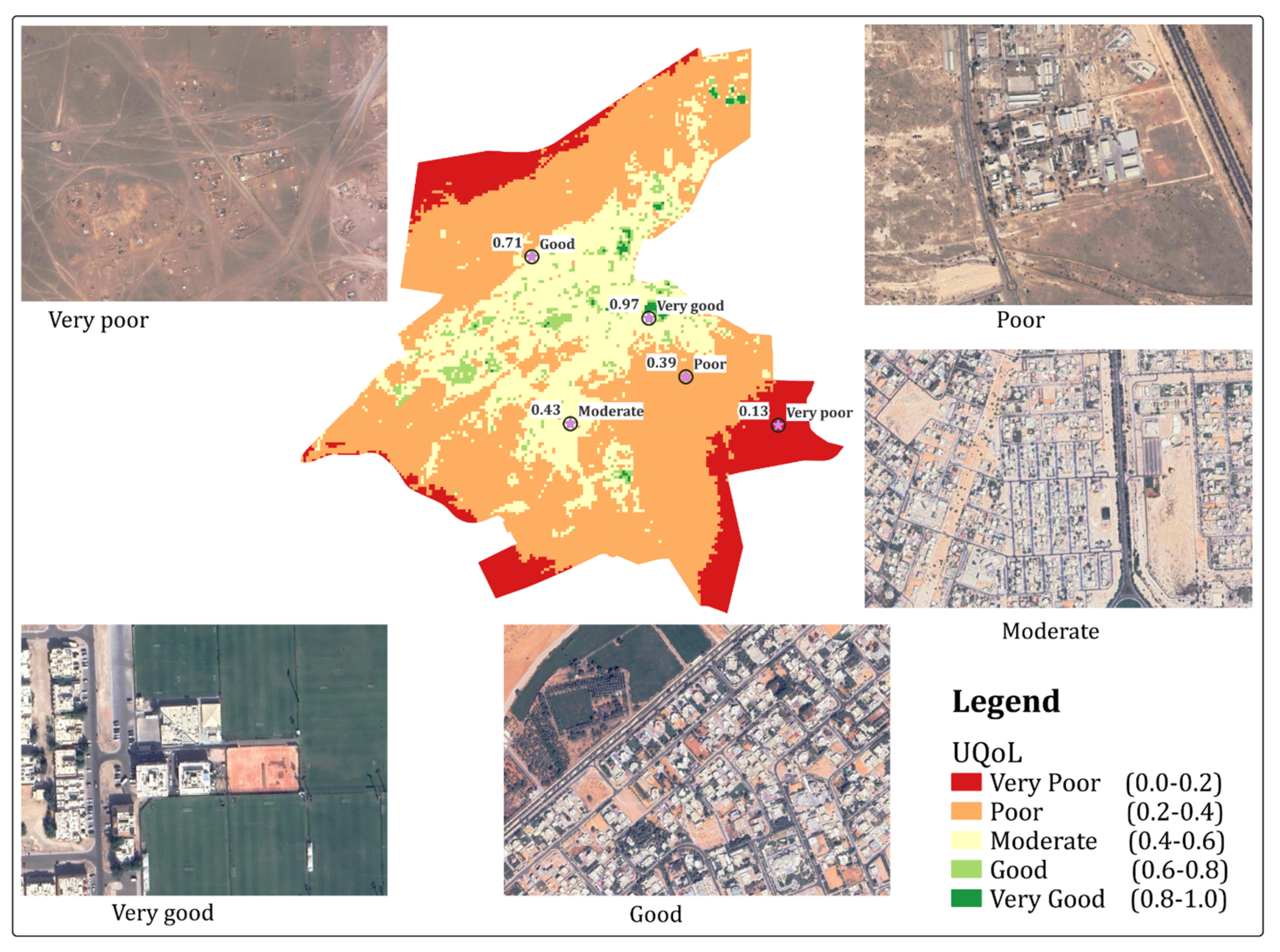
3.3. Urban Quality of Life Index (UQoL)
4. Discussion
5. Conclusions
Author Contributions
Funding
Institutional Review Board Statement
Informed Consent Statement
Data Availability Statement
Acknowledgments
Conflicts of Interest
Appendix A


References
- Liang, W.; Yang, M. Urbanization, economic growth and environmental pollution: Evidence from China. Sustain. Comput. Inform. Syst. 2019, 21, 1–9. [Google Scholar] [CrossRef]
- United Nations. 68% of the World Population Projected to Live in Urban Areas by 2050, Says UN|UN DESA|United Nations Department of Economic and Social Affairs [WWW Document]. United Nations. URL. 2018. Available online: https://www.un.org/development/desa/en/news/population/2018-revision-of-world-urbanization-prospects.html (accessed on 1 July 2022).
- Britt, C.L. Social context and racial disparities in punishment decisions. Justice Q. 2000, 17, 707–732. [Google Scholar] [CrossRef]
- Soh, M.B.C. Crime and Urbanization: Revisited Malaysian Case. Procedia—Soc. Behav. Sci. 2012, 42, 291–299. [Google Scholar] [CrossRef]
- Liang, L.; Wang, Z.; Li, J. The effect of urbanization on environmental pollution in rapidly developing urban agglomerations. J. Clean. Prod. 2019, 237, 117649. [Google Scholar] [CrossRef]
- Zhang, X.; Han, L.; Wei, H.; Tan, X.; Zhou, W.; Li, W.; Qian, Y. Linking urbanization and air quality together: A review and a perspective on the future sustainable urban development. J. Clean. Prod. 2022, 346, 130988. [Google Scholar] [CrossRef]
- Merschdorf, H.; Hodgson, M.E.; Blaschke, T. Modeling Quality of Urban Life Using a Geospatial Approach. Urban Sci. 2020, 4, 5. [Google Scholar] [CrossRef]
- Liang, B.; Weng, Q. Assessing Urban Environmental Quality Change of Indianapolis, United States, by the Remote Sensing and GIS Integration. IEEE J. Sel. Top. Appl. Earth Obs. Remote Sens. 2011, 4, 43–55. [Google Scholar] [CrossRef]
- Macke, J.; Casagrande, R.M.; Sarate, J.A.R.; Silva, K.A. Smart city and quality of life: Citizens’ perception in a Brazilian case study. J. Clean. Prod. 2018, 182, 717–726. [Google Scholar] [CrossRef]
- Mouratidis, K. Urban planning and quality of life: A review of pathways linking the built environment to subjective well-being. Cities 2021, 115, 103229. [Google Scholar] [CrossRef]
- Kazemzadeh-Zow, A.; Boloorani, A.D.; Samany, N.N.; Toomanian, A.; Pourahmad, A. Spatiotemporal modelling of urban quality of life (UQoL) using satellite images and GIS. Int. J. Remote Sens. 2018, 39, 6095–6116. [Google Scholar] [CrossRef]
- Bieda, A.; Telega, A. The Analysis of Research Hotspots in the Field of Urban Quality. Sustainability 2021, 13, 9582. [Google Scholar] [CrossRef]
- Pacione, M. Urban environmental quality and human wellbeing—A social geographical perspective. Landsc. Urban Plan. 2003, 65, 19–30. [Google Scholar] [CrossRef]
- Mostafa, A.M. Quality of Life Indicators in Value Urban Areas: Kasr Elnile Street in Cairo. Procedia—Soc. Behav. Sci. 2012, 50, 254–270. [Google Scholar] [CrossRef][Green Version]
- Seik, F.T. Subjective assessment of urban quality of life in Singapore (1997–1998). Habitat Int. 2000, 24, 31–49. [Google Scholar] [CrossRef]
- Yadav, J.; Gupta, N. Urban Quality of Life: Domains, Dimensions and Indicators for Indian Cities. IOP Conf. Ser. Earth Environ. Sci. 2021, 796, 012032. [Google Scholar] [CrossRef]
- Chen, S.; Cerin, E.; Stimson, R.; Lai, P. An Objective Measure to Assessing Urban Quality of Life based on Land Use Characteristics. Procedia Environ. Sci. 2016, 36, 50–53. [Google Scholar] [CrossRef]
- Al-Qawasmi, J.; Saeed, M.; Asfour, O.S.; Aldosary, A.S. Assessing Urban Quality of Life: Developing the Criteria for Saudi Cities. Front. Built Environ. 2021, 7, 682391. [Google Scholar] [CrossRef]
- Behling, R.; Bochow, M.; Foerster, S.; Roessner, S.; Kaufmann, H. Automated GIS-based derivation of urban ecological indicators using hyperspectral remote sensing and height information. Ecol. Indic. 2015, 48, 218–234. [Google Scholar] [CrossRef]
- de Deus, L.R.; Garcia Fonseca, L.M.; de Marcelhas e Souza, I. Creating an socio-environmental condition index to assess of urban environmental quality. In Proceedings of the Joint Urban Remote Sensing Event 2013, Sao Paulo, Brazil, 21–23 April 2013; pp. 271–274. [Google Scholar] [CrossRef]
- Huang, H.; Li, Q.; Zhang, Y. A High-Resolution Remote-Sensing-Based Method for Urban Ecological Quality Evaluation. Front. Environ. Sci. 2022, 10, 765604. [Google Scholar] [CrossRef]
- Nichol, J.; Wong, M.S. Mapping urban environmental quality using satellite data and multiple parameters. Environ. Plan. B Plan. Des. 2009, 36, 170–185. [Google Scholar] [CrossRef]
- Nichol, J.; Wong, M.S. Modeling urban environmental quality in a tropical city. Landsc. Urban Plan. 2005, 73, 49–58. [Google Scholar] [CrossRef]
- Han, P.; Zhang, Q.; Zhao, Y.; Li, F.Y. High-resolution remote sensing data can predict household poverty in pastoral areas, Inner Mongolia, China. Geogr. Sustain. 2021, 2, 254–263. [Google Scholar] [CrossRef]
- Rahman, M.; Szabó, G. Impact of Land Use and Land Cover Changes on Urban Ecosystem Service Value in Dhaka, Bangladesh. Land 2021, 10, 793. [Google Scholar] [CrossRef]
- Rahman, A.; Kumar, Y.; Fazal, S.; Bhaskaran, S. Urbanization and Quality of Urban Environment Using Remote Sensing and GIS Techniques in East Delhi-India. J. Geogr. Inf. Syst. 2011, 3, 62–84. [Google Scholar] [CrossRef]
- Macků, K.; Voženílek, V.; Pászto, V. Linking the quality of life index and the typology of European administrative units. J. Int. Dev. 2021, 34, 145–174. [Google Scholar] [CrossRef]
- Krishnan, V.S.; Firoz, C.M. Regional urban environmental quality assessment and spatial analysis. J. Urban Manag. 2020, 9, 191–204. [Google Scholar] [CrossRef]
- Wang, H.; Ma, C.; Zhou, L. A brief review of machine learning and its application. In Proceedings of the 2009 International Conference on Information Engineering and Computer Science, Wuhan, China, 19–20 December 2009. [Google Scholar] [CrossRef]
- Karita, S.; Watanabe, S.; Iwata, T.; Delcroix, M.; Ogawa, A.; Nakatani, T. Semi-supervised End-to-end Speech Recognition Using Text-to-speech and Autoencoders. In Proceedings of the ICASSP 2019 - 2019 IEEE International Conference on Acoustics, Speech and Signal Processing (ICASSP), Brighton, UK, 12–17 May 2019; pp. 6166–6170. [Google Scholar] [CrossRef]
- Jamtsho, T.; Powdyel, K.; Powrel, R.K.; Bhujel, R.; Muramatsu, K. OCR and Speech Recognition System Using Machine Learning. In Proceedings of the 2021 Innovations in Power and Advanced Computing Technologies (i-PACT), Kuala Lumpur, Malaysia, 27–29 November 2021. [Google Scholar] [CrossRef]
- Gao, Y.; Mas, J. A comparison of the performance of pixel based and object based classifications over images with various spatial resolutions. Online J. Earth Sci. 2008, 2, 27–35. [Google Scholar]
- Meneguzzo, D.M.; Liknes, G.C.; Nelson, M.D. Mapping trees outside forests using high-resolution aerial imagery: A comparison of pixel- and object-based classification approaches. Environ. Monit. Assess. 2012, 185, 6261–6275. [Google Scholar] [CrossRef]
- Balha, A.; Mallick, J.; Pandey, S.; Gupta, S.; Singh, C.K. A comparative analysis of different pixel and object-based classification algorithms using multi-source high spatial resolution satellite data for LULC mapping. Earth Sci. Inform. 2021, 14, 2231–2247. [Google Scholar] [CrossRef]
- Tassi, A.; Gigante, D.; Modica, G.; Di Martino, L.; Vizzari, M. Pixel- vs. Object-Based Landsat 8 Data Classification in Google Earth Engine Using Random Forest: The Case Study of Maiella National Park. Remote Sens. 2021, 13, 2299. [Google Scholar] [CrossRef]
- Nasir, S.M.; Kamran, K.V.; Blaschke, T.; Karimzadeh, S. Change of land use/land cover in kurdistan region of Iraq: A semi-automated object-based approach. Remote Sens. Appl. Soc. Environ. 2022, 26, 100713. [Google Scholar] [CrossRef]
- Tokar, O.; Vovk, O.; Kolyasa, L.; Havryliuk, S.; Korol, M. Using the Random Forest Classification for Land Cover Interpretation of Landsat Images in the Prykarpattya Region of Ukraine. In Proceedings of the 2018 IEEE 13th International Scientific and Technical Conference on Computer Sciences and Information Technologies (CSIT), Lviv, Ukraine, 11–14 September 2018; pp. 241–244. [Google Scholar] [CrossRef]
- Mansaray, L.R.; Wang, F.; Huang, J.; Yang, L.; Kanu, A.S. Accuracies of support vector machine and random forest in rice mapping with Sentinel-1A, Landsat-8 and Sentinel-2A datasets. Geocarto Int. 2019, 35, 1088–1108. [Google Scholar] [CrossRef]
- Breiman, L. Random forests. Mach. Learn. 2001, 45, 5–32. [Google Scholar] [CrossRef]
- Mountrakis, G.; Im, J.; Ogole, C. Support vector machines in remote sensing: A review. ISPRS J. Photogramm. Remote Sens. 2011, 66, 247–259. [Google Scholar] [CrossRef]
- Statistics Centre. Statistical Yearbook of Abu Dhabi 2020; Statistics Center: Abu Dhabi, The United Arab Emirates, 2020. [Google Scholar]
- Hejase, H.A.N.; Assi, A.H. Time-Series Regression Model for Prediction of Mean Daily Global Solar Radiation in Al-Ain, UAE, Time-series Regression Model for Prediction of Monthly and Daily Average Global Solar Radiation in Al Ain City—UAE. In Proceedings of the Global Conference on Global Warming 2011, Lisbon, Portugal, 11–14 July 2011. [Google Scholar]
- Yagoub, M.M. Parks in Al Ain, UAE: Geographical Distribution, Opportunities, and Challenges. Arab World Geogr. 2014, 17, 24–41. [Google Scholar]
- Yagoub, M.M.; Al Bizreh, A.A. Prediction of Land Cover Change Using Markov and Cellular Automata Models: Case of Al-Ain, UAE, 1992–2030. J. Indian Soc. Remote Sens. 2014, 42, 665–671. [Google Scholar] [CrossRef]
- Li, G.; Weng, Q. Measuring the quality of life in city of Indianapolis by integration of remote sensing and census data. Int. J. Remote Sens. 2007, 28, 249–267. [Google Scholar] [CrossRef]
- Chen, J.; Chen, S.; Yang, C.; He, L.; Hou, M.; Shi, T. A comparative study of impervious surface extraction using Sentinel-2 imagery. Eur. J. Remote Sens. 2020, 53, 274–292. [Google Scholar] [CrossRef]
- ESA. Aerosol Index—Level-2 Processing—Sentinel-5P Technical Guide—Sentinel Online—Sentinel Online [WWW Document]. The European Space Agency. URL. 2022. Available online: https://sentinels.copernicus.eu/web/sentinel/technical-guides/sentinel-5p/level-2/aerosol-index (accessed on 27 May 2022).
- Artis, D.A.; Carnahan, W.H. Survey of emissivity variability in thermography of urban areas. Remote Sens. Environ. 1982, 12, 313–329. [Google Scholar] [CrossRef]
- Xu, H. Modification of normalised difference water index (NDWI) to enhance open water features in remotely sensed imagery. Int. J. Remote Sens. 2006, 27, 3025–3033. [Google Scholar] [CrossRef]
- Zha, Y.; Gao, J.; Ni, S. Use of normalized difference built-up index in automatically mapping urban areas from TM imagery. Int. J. Remote Sens. 2003, 24, 583–594. [Google Scholar] [CrossRef]
- Richards, J.A.; Jia, X. Remote Sensing Digital Image Analysis, Remote Sensing Digital Image Analysis; Springer: Berlin/Heidelberg, Germany, 1999. [Google Scholar] [CrossRef]
- McFeeters, S.K. The use of the Normalized Difference Water Index (NDWI) in the delineation of open water features. Int. J. Remote Sens. 1996, 17, 1425–1432. [Google Scholar] [CrossRef]
- Huete, A.R. A soil-adjusted vegetation index (SAVI). Remote Sens. Environ. 1988, 25, 295–309. [Google Scholar] [CrossRef]
- Auquilla, A.; Heremans, S.; Vanegas, P.; Van Orshoven, J. A Procedure for Semi-automatic Segmentation in OBIA Based on the Maximization of a Comparison Index. In Computational Science and Its Applications—ICCSA; Springer: Cham, Switzerland, 2014; pp. 360–375. [Google Scholar] [CrossRef]
- Hay, G.J.; Castilla, G. Geographic object-based image analysis (GEOBIA): A new name for a new discipline. In Object-Based Image Analysis. Lecture Notes in Geoinformation and Cartography; Blaschke, T., Lang, S., Hay, G.J., Eds.; Springer: Berlin/Heidelberg, Germany, 2008; pp. 75–89. [Google Scholar] [CrossRef]
- Sapena, M.; Wurm, M.; Taubenböck, H.; Tuia, D.; Ruiz, L.A. Estimating quality of life dimensions from urban spatial pattern metrics. Comput. Environ. Urban Syst. 2020, 85, 101549. [Google Scholar] [CrossRef]
- Faisal, K.; Shaker, A. An Investigation of GIS Overlay and PCA Techniques for Urban Environmental Quality Assessment: A Case Study in Toronto, Ontario, Canada. Sustainability 2017, 9, 380. [Google Scholar] [CrossRef]
- Jolliffe, I.T. Principal Component Analysis, 2nd ed.; Springer-Verlag Inc.: New York, NY, USA, 2002. [Google Scholar]
- Musse, M.A.; Barona, D.A.; Rodriguez, L.M.S. Urban environmental quality assessment using remote sensing and census data. Int. J. Appl. Earth Obs. Geoinf. 2018, 71, 95–108. [Google Scholar] [CrossRef]
- Addas, A. Exploring the pattern of use and accessibility of urban green spaces: Evidence from a coastal desert megacity in Saudi Arabia. Environ. Sci. Pollut. Res. 2022, 29, 55757–55774. [Google Scholar] [CrossRef]
- Khalil, H.A.E.E. Enhancing quality of life through strategic urban planning. Sustain. Cities Soc. 2012, 5, 77–86. [Google Scholar] [CrossRef]
- Ma, L.; Liu, S.; Fang, F.; Che, X.; Chen, M. Evaluation of urban-rural difference and integration based on quality of life. Sustain. Cities Soc. 2019, 54, 101877. [Google Scholar] [CrossRef]
- Markevych, I.; Schoierer, J.; Hartig, T.; Chudnovsky, A.; Hystad, P.; Dzhambov, A.M.; de Vries, S.; Triguero-Mas, M.; Brauer, M.; Nieuwenhuijsen, M.J.; et al. Exploring pathways linking greenspace to health: Theoretical and methodological guidance. Environ. Res. 2017, 158, 301–317. [Google Scholar] [CrossRef]
- Thangiah, G.; Said, M.A.; Majid, H.A.; Reidpath, D.; Su, T.T. Income Inequality in Quality of Life among Rural Communities in Malaysia: A Case for Immediate Policy Consideration. Int. J. Environ. Res. Public Health 2020, 17, 8731. [Google Scholar] [CrossRef] [PubMed]
- Giannico, V.; Spano, G.; Elia, M.; D’Este, M.; Sanesi, G.; Lafortezza, R. Green spaces, quality of life, and citizen perception in European cities. Environ. Res. 2021, 196, 110922. [Google Scholar] [CrossRef] [PubMed]
- Rahman, M.; Szabó, G. A Novel Composite Index to Measure Environmental Benefits in Urban Land Use Optimization Problems. ISPRS Int. J. Geo-Inf. 2022, 11, 220. [Google Scholar] [CrossRef]


| Indicator | Equation | No. | Reference | Format |
|---|---|---|---|---|
| AI * | 1 | [47] | Raster | |
| ENDISI * | 2 | [46] | Raster | |
| LST * | 3 | [48] | Raster | |
| MNDWI * | 4 | [49] | Raster | |
| NDBI * | 5 | [50] | Raster | |
| NDVI * | 6 | [51] | Raster | |
| NDWI * | 7 | [52] | Raster | |
| Slope * | 8 | Raster | ||
| SAVI * | 9 | [53] | Raster | |
| LULC * | OBIA-RF | 10 | Vector | |
| Built-up to baren soil ratio * | 11 | Vector | ||
| Built-up to green area ratio * | 12 | Vector | ||
| Distance to main road † | Vector | |||
| Distance to park † | Vector | |||
| Distance to school † | Vector | |||
| Distance of hospital † | Vector |
| Class Value | Built-Up | Bare Soil | Green Area | Highland | Total |
|---|---|---|---|---|---|
| Built-up | 9099 | 1068 | 403 | 13 | 10,583 |
| Bare soil | 369 | 147,283 | 992 | 715 | 149,359 |
| Green area | 26 | 71 | 29,997 | 0 | 30,094 |
| Highland | 0 | 237 | 21 | 14,450 | 14,708 |
| Total | 9494 | 148,659 | 31,413 | 15,178 | 204,744 |
| PA (%) | 99.4 | 95.2 | 88.7 | 94.7 | |
| UA (%) | 86.0 | 98.6 | 99.7 | 98.2 | |
| Kappa hat | 0.82 | 0.97 | 0.99 | 0.98 | |
| Overall accuracy | 95.3 | ||||
| Kappa hat classification | 0.92 | ||||
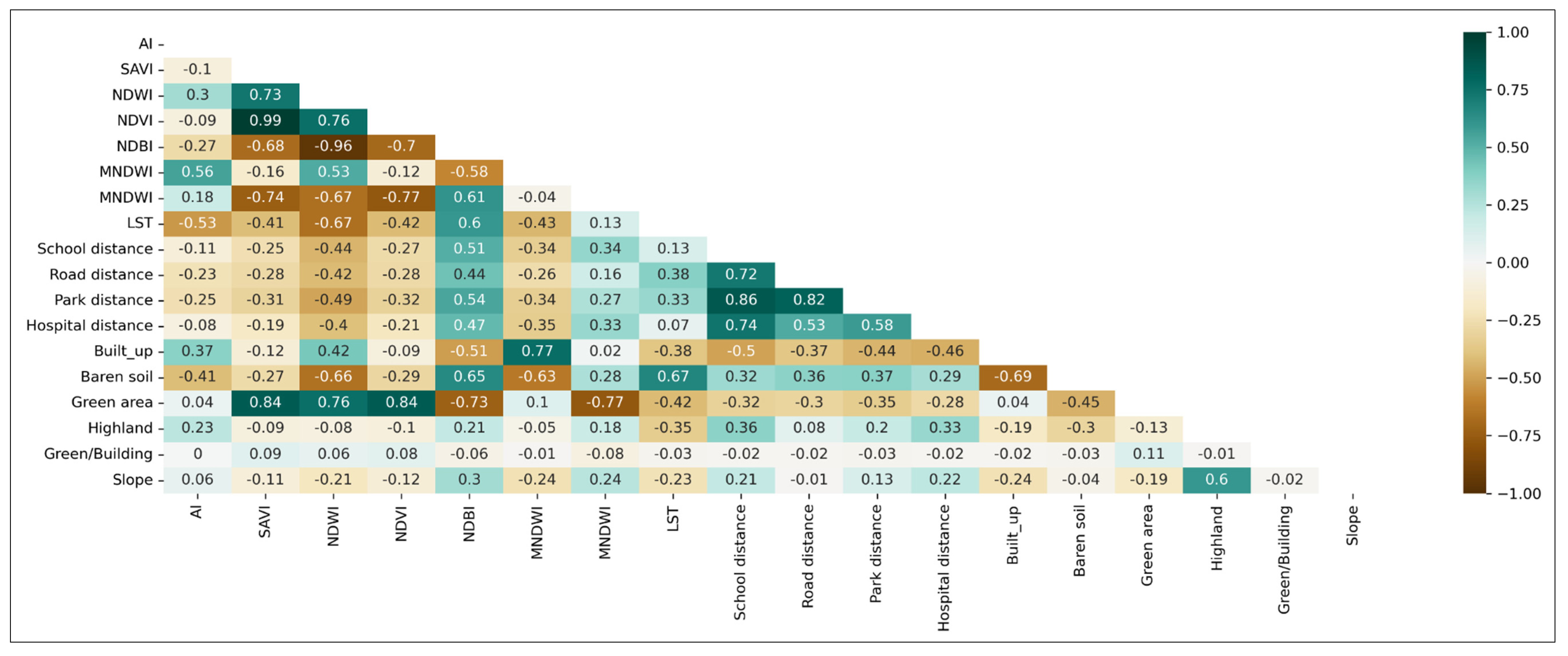
| Mean | Std | Min | Max | |
|---|---|---|---|---|
| AI | 0.08 | 0.13 | −0.16 | 0.36 |
| SAVI | 0.09 | 0.07 | −0.20 | 0.68 |
| NDWI | −0.05 | 0.09 | −0.57 | 0.73 |
| NDVI | 0.10 | 0.07 | −0.31 | 0.76 |
| NDBI | 0.10 | 0.08 | −0.65 | 0.49 |
| MNDWI | −0.33 | 0.09 | −0.62 | 0.37 |
| ENDISI | −0.13 | 0.13 | −0.74 | 0.52 |
| LST | 43.16 °C | 13 °C | 31.37 °C | 48.12 °C |
| Slope | 4.95 | 5.48 | 0 | 68.86 |
| Distance to school | 4080 m | 3167 m | 0 | 15,134 m |
| Distance to road | 1654 m | 1835 m | 0 | 10,191 m |
| Distance to park | 4112 m | 2769 m | 0 | 14,270 m |
| Distance to hospital | 8325 m | 4561 m | 0 | 21,340 m |
| Built-Up Area | Baren-Soil Area | Green Area | Highland Area | |
|---|---|---|---|---|
| AI | 0.37 *** | −0.41 *** | 0.04 *** | 0.23 *** |
| SAVI | −0.12 *** | −0.27 *** | 0.84 *** | −0.09 *** |
| NDWI | 0.42 *** | −0.66 *** | 0.76 *** | −0.08 *** |
| NDVI | −0.09 *** | −0.29 *** | 0.84 *** | −0.10 *** |
| NDBI | 0.51 *** | 0.65 *** | −0.73 *** | 0.21 *** |
| MNDWI | 0.77 *** | −0.63 *** | 0.1 *** | −0.05 *** |
| ENDISI | 0.02 * | 0.28 *** | −0.77 *** | 0.18 *** |
| LST | −0.38 *** | 0.67 *** | −0.42 *** | −0.35 *** |
| Slope | −0.24 *** | −0.04 *** | −0.19 *** | 0.6 *** |
| Distance to school | −0.5 *** | 0.32 *** | −0.32 *** | 0.36 *** |
| Distance to road | −0.37 *** | 0.36 *** | −0.3 *** | 0.08 *** |
| Distance to park | −0.44 *** | 0.37 *** | −0.35 *** | 0.20 *** |
| Distance to hospital | −0.46 *** | 0.29 *** | −0.28 *** | 0.33 *** |
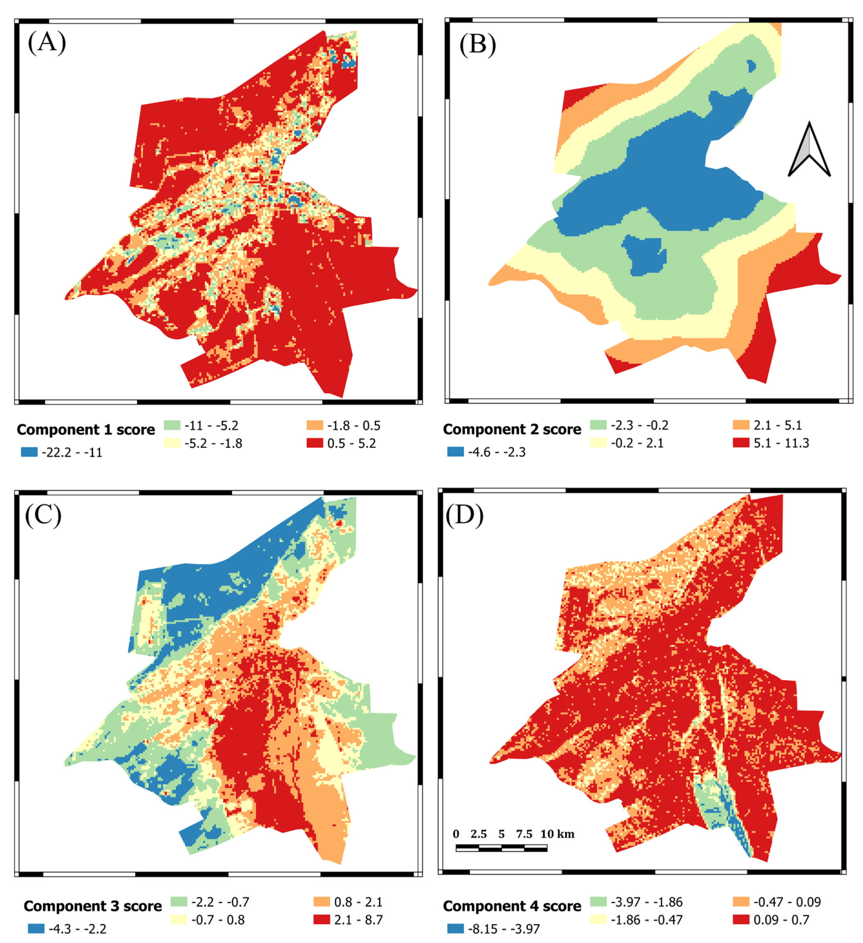
| ID | Variables | Components and Loadings | |||
|---|---|---|---|---|---|
| 1 | 2 | 3 | 4 | ||
| 1 | AI | 0.153 | −0.093 | 0.838 | 0.034 |
| 2 | SAVI | −0.963 | −0.147 | −0.019 | 0.108 |
| 3 | NDWI | −0.764 | −0.281 | 0.522 | −0.199 |
| 4 | NDVI | −0.969 | −0.155 | 0.001 | 0.08 |
| 5 | NDBI | 0.699 | 0.349 | −0.494 | 0.304 |
| 6 | MNDWI | 0.088 | −0.228 | 0.78 | −0.483 |
| 7 | ENDISI | 0.828 | 0.177 | 0.123 | 0.241 |
| 8 | LST | 0.398 | 0.107 | −0.783 | −0.321 |
| 9 | Slope | 0.145 | 0.053 | 0.094 | 0.862 |
| 10 | Distance to school | 0.147 | 0.92 | −0.05 | 0.202 |
| 11 | Distance to main road | 0.132 | 0.86 | −0.217 | −0.178 |
| 12 | Distance to park | 0.182 | 0.892 | −0.211 | 0.011 |
| 13 | Distance to hospital | 0.127 | 0.753 | −0.034 | 0.335 |
| 14 | Green to build-up ratio | −0.123 | 0.001 | −0.01 | 0.004 |
| 15 | Building to bare soil ratio | 0.02 | −0.04 | 0.084 | −0.103 |
| Initial eigenvalues | 5.757 | 2.424 | 1.815 | 1.298 | |
| Eigenvalues after Varimax rotation | 3.938 | 3.305 | 2.566 | 1.484 | |
| % Of variance | 26.26 | 22.03 | 17.11 | 9.90 | |
| Cumulative variance | 26.26 | 48.29 | 65.40 | 75.29 | |
| Weights calculated (%) | 34.88 | 29.20 | 22.72 | 13.11 | |
| Independent Variable | Dependent Variable | Loadings | R2 | Constant | Coefficient |
|---|---|---|---|---|---|
| Component 1 score | NDVI | −0.97 | 0.96 * | −2.91 × 10¹⁶ | −0.36 |
| Component 2 score | Distance to school | 0.92 | 0.89 * | 4.07 × 10¹⁶ | 0.31 |
| Component 3 score | Aerosol index | 0.84 | 0.74 * | 1.57 × 10¹⁵ | 0.44 |
Publisher’s Note: MDPI stays neutral with regard to jurisdictional claims in published maps and institutional affiliations. |
© 2022 by the authors. Licensee MDPI, Basel, Switzerland. This article is an open access article distributed under the terms and conditions of the Creative Commons Attribution (CC BY) license (https://creativecommons.org/licenses/by/4.0/).
Share and Cite
Yagoub, M.M.; Tesfaldet, Y.T.; Elmubarak, M.G.; Al Hosani, N. Extraction of Urban Quality of Life Indicators Using Remote Sensing and Machine Learning: The Case of Al Ain City, United Arab Emirates (UAE). ISPRS Int. J. Geo-Inf. 2022, 11, 458. https://doi.org/10.3390/ijgi11090458
Yagoub MM, Tesfaldet YT, Elmubarak MG, Al Hosani N. Extraction of Urban Quality of Life Indicators Using Remote Sensing and Machine Learning: The Case of Al Ain City, United Arab Emirates (UAE). ISPRS International Journal of Geo-Information. 2022; 11(9):458. https://doi.org/10.3390/ijgi11090458
Chicago/Turabian StyleYagoub, Mohamed. M., Yacob T. Tesfaldet, Marwan G. Elmubarak, and Naeema Al Hosani. 2022. "Extraction of Urban Quality of Life Indicators Using Remote Sensing and Machine Learning: The Case of Al Ain City, United Arab Emirates (UAE)" ISPRS International Journal of Geo-Information 11, no. 9: 458. https://doi.org/10.3390/ijgi11090458
APA StyleYagoub, M. M., Tesfaldet, Y. T., Elmubarak, M. G., & Al Hosani, N. (2022). Extraction of Urban Quality of Life Indicators Using Remote Sensing and Machine Learning: The Case of Al Ain City, United Arab Emirates (UAE). ISPRS International Journal of Geo-Information, 11(9), 458. https://doi.org/10.3390/ijgi11090458