Article

Liquefaction Potential and Vs30 Structure in the Middle-Chelif Basin, Northwestern Algeria, by Ambient Vibration Data Inversion

by
Abdelouahab Issaadi
1,2,*,
Ahmed Saadi
1,2,
Fethi Semmane
1,
Abdelkrim Yelles-Chaouche
1 and
Juan José Galiana-Merino
2,3
1
Centre de Recherche en Astronomie, Astrophysique et Géophysique (CRAAG), Algiers 16340, Algeria
2
University Institute of Physics Applied to Sciences and Technologies, University of Alicante, 03080 Alicante, Spain
3
Departement of Physics, Systems Engineering and Signal Theory, University of Alicante, 03080 Alicante, Spain
*
Author to whom correspondence should be addressed.
Appl. Sci. 2022, 12(16), 8069; https://doi.org/10.3390/app12168069
Submission received: 28 June 2022 / Revised: 29 July 2022 / Accepted: 1 August 2022 / Published: 12 August 2022
(This article belongs to the Special Issue Geohazards: Risk Assessment, Mitigation and Prevention)

Abstract

:
The Middle-Chelif basin, in northwestern Algeria, is located in a seismically active region. In its western part lies the El-Asnam fault, a thrust fault responsible for several strong earthquakes. The most important being the El-Asnam earthquake (Ms = 7.3) of 1980. In the present study, ambient vibration data with single-station and array techniques were used to investigate the dynamic properties of the ground and to estimate the V s 30 structure in the main cities of the basin. Soil resonance frequencies vary from 1.2 to 8.3 Hz with a maximum amplitude of 8.7 in. Collapsing behavior has also been demonstrated west of the city of El-Attaf, reflecting a strong potential for liquefaction. A V s 30 variation map and a soil classification for each city were obtained mainly by inversion of the HVSR and Rayleigh wave dispersion curves. Finally, an empirical prediction law of V s 30 for the Middle-Chelif basin was proposed.

1. Introduction

Northern Algeria is located in the collision zone between the African and Eurasian plates. It is characterized by moderate to high seismic activity (e.g., [1,2,3]), mainly concentrated in the marginal areas of the Neogene basins [4]. The Chelif Basin is located in the northwestern part of Algeria (Figure 1). It is the largest of the northern Neogene sedimentary basins and hosts an important seismic activity. The basin is mainly affected by NE-SW oriented reverse faults [4,5]. The most important is the El-Asnam fault, a reverse fault about 40 km long [6], that generated several destructive earthquakes during the last century, such as the 1934 Carnot earthquake, now El-Abadia, ( M S = 5.1, [7]); the 1954 Orléansville earthquake, now Chlef (MS = 6.7, [7]); and the 1980 El-Asnam earthquake, now Chlef (MS = 7.3, [6]). The latter is the largest and most destructive earthquake recorded in Algeria in the instrumental era.
The Chelif Basin is divided into three parts: the Lower-Chelif Basin, the Middle-Chelif Basin, and the Upper-Chelif Basin. The Middle-Chelif extends from Oued-Fodda in the west to Ain-Defla in the east (Figure 1). The cities of the Middle-Chelif suffered important damage during the 1980 El-Asnam earthquake. The cities of Oued-Fodda, El-Abadia, and El-Attaf were almost totally destroyed. In addition, several secondary effects of the earthquake were observed along the rupture zone [8], such as cracks, settlement, and soil liquefaction. Moreover, the coseismic uplift of the western part of the fault has obstructed the flow of the Chelif River, causing a flood which formed a natural dam, where the phenomenon of liquefaction occurred over a wide area west of El-Abadia and El-Attaf [8,9].
Prior to the 1980 El-Asnam earthquake, several geological and geophysical studies were conducted on the Chelif Basin (e.g., [10,11]). However, these studies were mainly concentrated in the Lower-Chelif Basin due to the presence of oil indices. Only a few studies have been carried out on the Middle-Chelif Basin [12,13]. Right after the 1980 earthquake and given the extent of its damage, the region has finally been the subject of several geological, seismological, and geophysical studies (e.g., [6,8,14,15]). The firm Woodward and Clyde Consultants [15] conducted an important seismic microzonation study in eight cities of the Lower and Middle-Chelif Basins, including El-Abadia and El-Attaf. During the investigations, several holes were drilled using Standard Penetration Tests (SPT). The study provided geotechnical, hydrogeological, landslide, and liquefaction potential maps for each of the eight cities. The Neogene formations of the Middle-Chelif were described in detail in [12], and later in [16]. Furthermore, the structural aspect of the shallow and deep lithological units was recently imaged using land gravity data [17].
In the present study, we used ambient vibrations data to characterize some geotechnical features and to estimate some dynamic properties of the soil column in the cities of El-Attaf, El-Abadia, and Ain-Defla. Ambient vibration-based techniques have been used previously in the Chelif Basin [18,19,20,21]. The aim was to determine the resonance frequencies of the ground, the shear-wave velocity structure of the sedimentary layers, and the bedrock depth, where the impedance contrasts with the sedimentary cover and may be the cause for ground shaking amplification during strong earthquakes. This work is a continuation of the ones carried out in the Middle-Chelif basin [20,21].
In the first part of this study, we used ambient vibration data recorded from single stations to estimate the ground resonance frequencies and assess the liquefaction potential in the three cities under study. In the second part, we used ambient vibration data recorded from single station and array techniques to estimate the average shear-wave velocity in the upper 30 m of the soil column ( V s 30 ). Finally, a V s 30 predictive equation for the Middle-Chelif Basin was proposed.
This study contributes to the seismic hazard assessment in northern Algeria. The results obtained in this work can be used for ground motion simulation, for the calculation of amplification factors, and for many other studies related to the reduction of seismic risk.

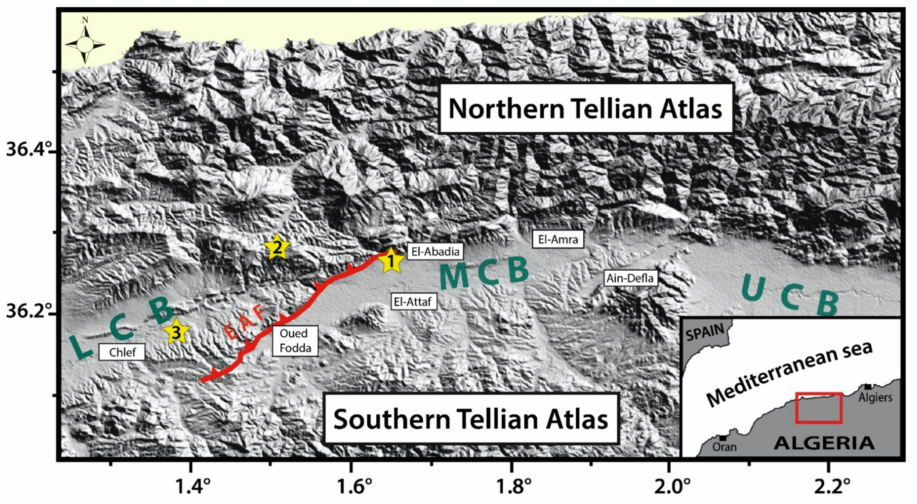
2. Geological Framework

The Middle-Chelif is an intra-mountainous basin structured during the Neogene [5,10,12], and located within the Tellian Atlas mountain belts (Figure 1). The depression is filled with a thick cover of Mio-Plio-Quaternary sediments. The basement is composed of hard clays and marls of Cretaceous age [12,16]. In its southern part, autochthonous formations of Jurassic to Silurian age outcrop [22], and form the Temoulga, Rouina, and Doui massifs (Figure 2). The Middle-Chelif plain is crossed from west to east by the Cheliff River, the longest in Algeria, which contributes to form the actual alluviums.
The stratigraphical column is composed of a succession of marine, continental, and lacustrine deposits. Lateral variations in facies were also reported [10,16], and further confirmed in [21], where important lateral variations in the shear-wave velocity were observed within the same formations. All these perturbations in the sedimentary cover reflect several instability periods with intense tectonic activities and different episodes of marine regression and transgression that conditioned the sedimentation process [10]. However, the geologists are not in agreement concerning the age of the first sedimentary deposits. Some authors attributed those sediments to the Lower Miocene [10,12], while others assigned them to the Middle Miocene (Serravallo-Tortonian) [16,23]. The sediments are affected by a series of normal and thrust faults, located in the margins of the Middle-Chelif Plain.
In terms of lithology, the Miocene series occupies the major part of the sedimentary column. These formations were described and detailed in [12]. The first deposits are detritic continental series of conglomerates and marls. These sediments are overlayed by different intercalations of marls, clays, limestones, and sandstones [12,16]. A thin layer of blue marls marks the transition between the Miocene and the Pliocene sediments [10,12]. The Miocene series outcrop in succession on the hills that overlook the city of El-Abadia (Figure 2). The shear-wave velocity varies from 640 to 1450 m/s for the Miocene formations [21]. The Pliocene is divided in two stages, marine and continental, with alternations between sands, sandstones, and conglomerates [10,16]. The Quaternary deposits are continental and predominant in the Middle-Chelif Plain. They are represented by Holocene and Pleistocene alluviums.
The three cities under study are built on Quaternary alluviums of different thicknesses. The city of Ain-Defla is built at the bottom of the northern flank of the Doui massif (Figure 2), where the topmost layer of the soil is composed of old Quaternary clays and gravels (Pleistocene), reaching a maximum thickness of 60 m [21]. The old alluviums lay directly over hard Jurassic limestone and Silurian schists and quartzite [22].
The cities of El-Attaf and El-Abadia are built on stiff Quaternary soil, the topmost layer is thin (<20 m) [21], and composed of recent alluviums (Holocene), which lie over older alluviums (Pleistocene). The engineering bedrock in El-Abadia is composed of Pliocene sandstones, while in El-Attaf, it is composed of Miocene marls and sandstones [14,21]. In these cases, the engineering bedrock has been characterized as the first layer of the soil column that contains a shear-wave velocity value above 750 m/s.
The presence of important sandbanks at shallow depths (<10 m) in El-Attaf and El-Abadia may lead to liquefaction phenomena during ground shaking. The risk is weak in El-Abadia since the sandy layers are dense and the ground water level is between 15 and 30 m deep [15]. However, in El-Attaf the risk is significant since the sandy banks are loose and the ground water level is shallow (between 7 and 10 m) [15].

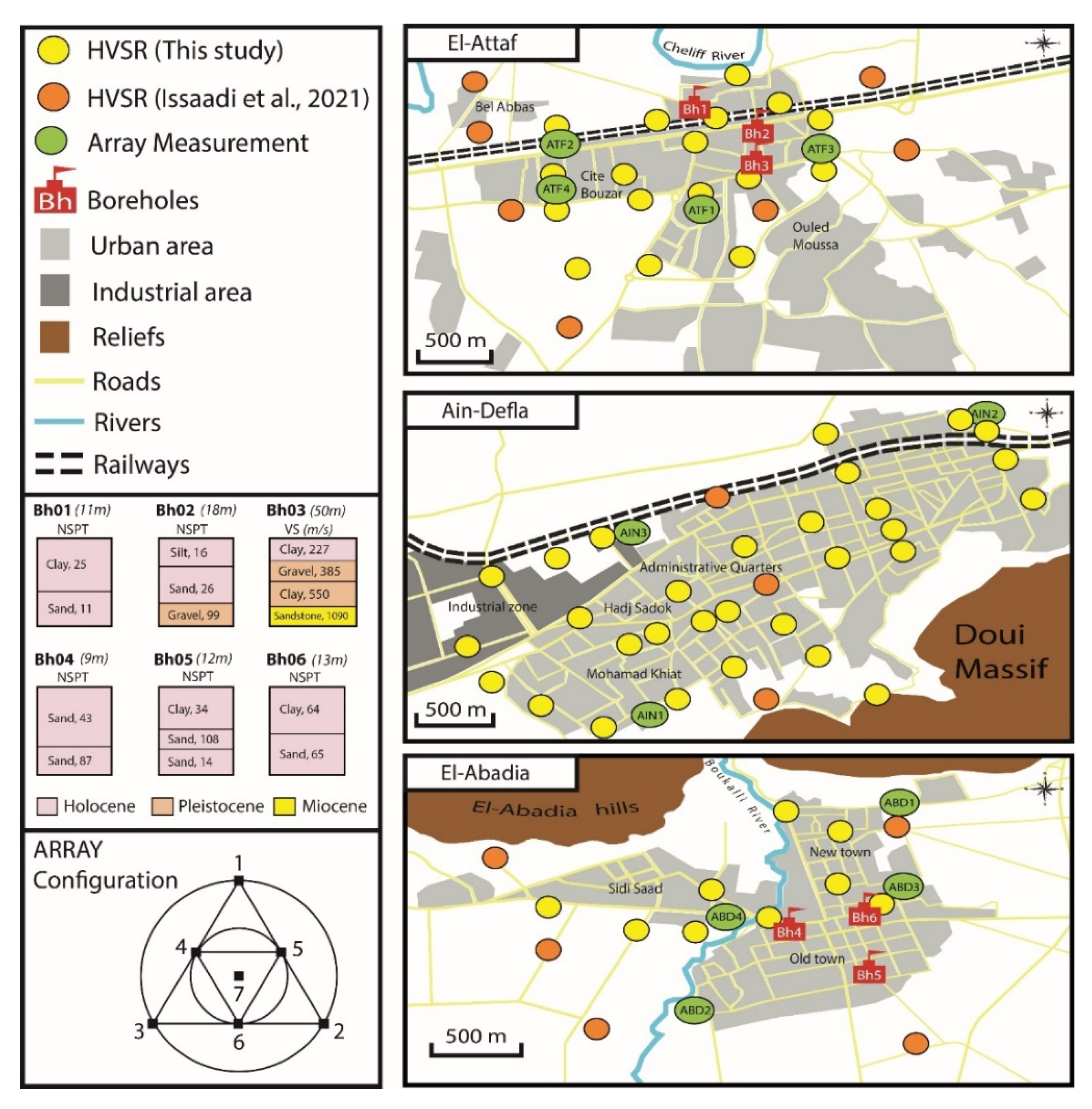
3. Data and Methodology

3.1. Horizontal-to-Vertical Spectral Ratio Technique (HVSR)

The HVSR (or H/V) technique [25] allows retrieval of the resonance frequency of the soil at a given site, using single station ambient vibrations measurements. The theoretical aspect of this technique consists of calculating the ratio between the amplitude spectra of the vertical and horizontal components of ambient vibrations. As a result, an HVSR curve is obtained. The HVSR frequency peak is well correlated with the soil resonance frequency.
Although this technique is very effective in estimating the soil resonance frequency [26], the scientific community is reluctant about its ability to estimate the amplification factors [27,28,29]. This issue is due to the contribution of different seismic waves to the wavefield. As for now, it is very difficult to quantify the ratio between body and surface waves. Bonnefoy-Claudet et al. [30] showed that in the case of high impedance contrasts between the bedrock and the sediments, the HVSR curve is mainly controlled by surface waves. The relatively low amplitude of the body waves is not sufficient to correctly estimate the amplification factor. Moreover, La Rocca et al. [31] and Benkaci et al. [32] have proven that the HVSR peak amplitude varies considerably with time. The amplitude of the frequency peak obtained from the HVSR technique in this study is interpreted as a relative indicator and not as a true amplification factor value.
Ambient vibration single-station measurements were carried out in October 2021 at 71 sites in the cities of El-Attaf (24 sites), Ain-Defla (33 sites), and El-Abadia (14 sites) (Figure 3). Some measurement points [15] were taken from a previous study [21]. Recordings were performed at night and in calm weather, as recommended by the SESAME project [33]. The acquisition time was 20 min. At some sites, the recording time was extended to 30 min due to anthropogenic noise from human activity. The equipment used for the recording was a pair of Tromino seismographs, with a sampling rate of 512 samples per second.
The HVSR technique was processed following the recommendations of the SESAME project [33]. The whole data were processed in the same way using the Geopsy software [34]. First, the signals were divided into several windows of 30 s each, tapered by a 5% cosine function. The window selection was made automatically using an anti-triggering algorithm, which allows selecting windows where the ambient noise is stationary. After that, the Fast Fourier Transform (FFT) is computed for each component (vertical and both horizontals) and the amplitude spectrum of both horizontal components is combined by an RMS (root mean square) average computation. After that, the ratio between the amplitude spectrum of both vertical and horizontal components is calculated. The HVSR curve is calculated for each window. The resulting curve is smoothed using the Konno–Ohmachi algorithm [35], with a smoothing coefficient of 40. Finally, the curves are averaged and the final HVSR curve is retrieved in the frequency range between 0.2 and 20 Hz. The resulting HVSR curve may contain one or several frequency peaks, which are directly linked to impedance contrasts at the soil column.

3.2. Seismic Vulnerability Index (Kg) and Shear Strain (Υ)

The stability of structures during an earthquake depends on the behavior of the ground, which in turn depends on the dynamic properties of the soil column. Ishihara [36] established a relation between the shear strain deformation and the dynamic properties of the soil, by compiling several earthquake data, reports, and laboratory tests (Table 1). Nakamura [37] introduced a method based on the vulnerability index calculation using ambient vibration data to estimate the shear strain, for the purpose of potential earthquake damage assessment (soil liquefaction, landslides).
The vulnerability index is calculated using the following equation [37]:
K g = e × ( A g 2 F g ) ( π 2 × V b )
where Fg is the resonance frequency of the soil, and Ag is the corresponding amplitude obtained with HVSR method. Vb is the velocity at the bedrock and e is the applied dynamic force. According to Nakamura [37], where several values of dynamic force were applied and tested with several velocity values for bedrock, the optimal results are obtained with an applied dynamic force of 60%. Thus, assuming this value and a velocity at the bedrock around 6 × 104 cm/s [37], Equation (1) can then be simplified as follows:
K g = ( A g 2 F g ) × 10 6
The shear strain can then be calculated by multiplying the vulnerability index (Kg) with the maximum observed acceleration, or the peak ground acceleration (αg) [37].
Υ   =   K g × α g
where the αg value is in cm/s2 (Gal). The peak ground acceleration values for El-Attaf and El-Abadia cities are 410 and 520 cm/s2, respectively, for a return period of 500 years [15]. For Ain-Defla city, a value of 250 cm/s2 is proposed [38].
This technique is used in the present work mainly to assess the liquefaction potential in the study area. For a shear strain value Υ > 10−2, phenomena of liquefaction and landslides are likely to occur during earthquakes.

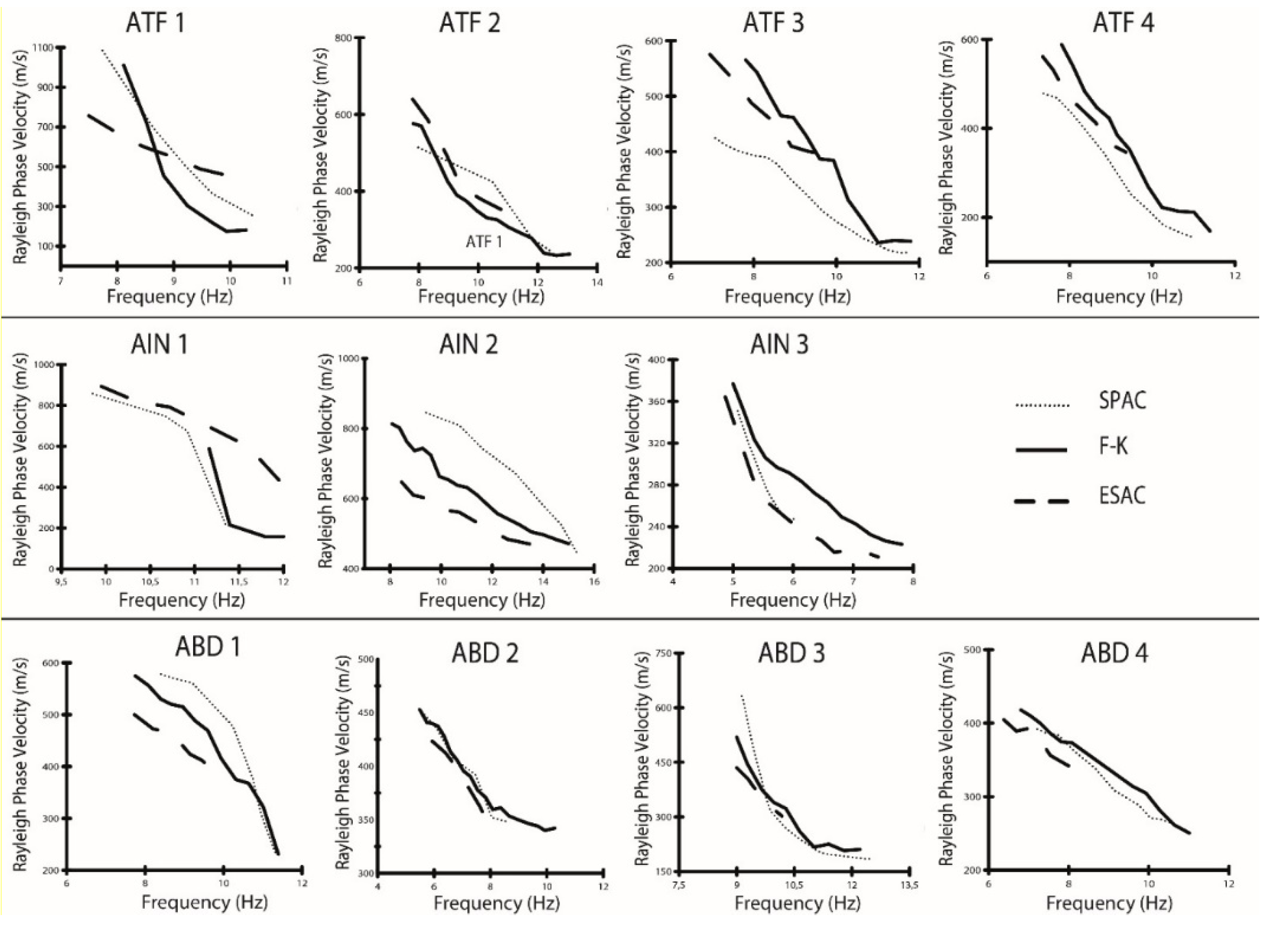
3.3. Array Techniques

Array-based techniques allow to obtain surface wave dispersion curves from ambient vibration records. In this study, three array techniques were used to extract the Rayleigh wave dispersion curves: the frequency-wavenumber (F-K) analysis [39,40,41,42], the spatial auto-correlation (SPAC) technique [43,44,45], and the extended spatial auto-correlation (ESAC) technique [44,46]. Some assumptions about the soil conditions are required before using these techniques. For example, it is assumed that the ambient vibration wavefield is essentially dominated by surface waves (especially the fundamental mode), and that the subsurface layers are homogenous and horizontally stratified, which means that in each layer the seismic waves propagate at a constant velocity [44].
The array measurement campaign was carried out in January 2021. The difficulty of finding open fields far enough from human activities inside urban areas, limited the measurement sites to 11 (four in El-Attaf and El-Abadia, and three in Ain-Defla). The measurements were made during daytime with a recording time of 40 min. The configuration of the array is triangular. Concretely, the sensor deployment consists of an equilateral triangle of 30 m on each side, with a sensor placed at each vertex, a sensor placed midway on each side, and an additional sensor placed at the center (Figure 3). This configuration provides a better coverage. According to [44], the equilateral triangle is the most efficient configuration for array techniques. The equipment used was formed by 7 SARA SS10 triaxial velocity sensors (f0 = 1 Hz) connected to SL06 digitizers.

3.3.1. The Frequency-Wavenumber (F-K) Analysis

F-K analysis is one of the most commonly used techniques for estimating Rayleigh wave dispersion curves. It has some advantages over other techniques, such as the ability to identify the direction of ambient vibration source and the recognition of the different modes presented in the wavefield [47]. The latter is composed of a superposition of several propagated waves. The F-K technique allows estimating the velocity and the direction of approach (back-azimuth) of these waves [48].
The F-K technique is based on two fundamental assumptions: the first is that the process is stationary in time. The second is that the process is stationary in the horizontal plane and that the propagation of the wavefront is only in the vertical direction. The stationary aspect of propagated seismic waves allows the power spectral density function of the frequency wavenumber to be calculated, which contains information about the power as a function of frequency and velocity vectors of the propagated wave. There are two methods for calculating the power spectral density: the maximum likelihood method (MLM) or the high-resolution method [40,41] and the beamforming method (BFM) [42]. The BFM technique is used in this study, as it is less sensitive to errors than the MLM technique [41].
For all the array techniques, only the vertical component of the records was analyzed, as it is the one required for the estimation of the Rayleigh wave dispersion curves. The Sesarray software package [34] was used to perform the F-K analysis. First, the coordinates of each of the seven sensors were introduced in the WARANGPS software in order to calculate the array transfer function and the theoretical wavenumber limits (Kmin and Kmax). Then, the signals were loaded into the Geopsy software and the BFM method was applied. The signals were divided into several windows of frequency-dependent lengths (50 periods). After that, an anti-triggering algorithm was used for the window selection. The processing requires the input of the grid step and grid size parameters. The grid size corresponds to the Kmax value, which is related to the aliasing limit. The grid step determines the maximum resolution and was chosen as Kmin/2. Once all these parameters were introduced, the final processing was launched and the dispersion curve was obtained. The processing was the same for the data of the 11 arrays.

3.3.2. The SPAC and ESAC Techniques

The spatial auto-correlation and the extended spatial auto-correlation techniques are based on the assumption of a stochastic wavefield being stationary both in space and time [43].
In theory, the SPAC technique consists of calculating a single-phase velocity value at each frequency in a predefined frequency band by fitting the SPAC coefficient to a Bessel function. For a circular array, the Bessel function represents the average cross-correlation between pairs of stations as a function of their distance. Aki [43] showed that the SPAC coefficient at a given frequency has the same form as the 0th order Bessel function.
The SPAC method requires a circular array configuration with a centrally located sensor [44]. A modification of this technique has been suggested by Bettig et al. [45], which allows the SPAC technique to be applied to arrays of arbitrary configuration. The modification consists of replacing the use of fixed radius values with rings of finite thickness.
The ESAC method differs from SPAC by fixing the frequency values instead of the radius. At each frequency, the normalized transverse spectrum is fitted to the Bessel function. The inverted Bessel function that has the best fit with the normalized cross-spectra allows to obtain the phase velocity [46].
As with the F-K analysis, the SPAC technique was performed using the SESARRAY software package [34]. The first step is to define the ring parameters using the SPAC toolbox of the Geopsy software. Once the coordinates of the sensors are entered, the software will define a set of spatially distributed sensor pairs (e.g., 21 pairs for 7 sensors). Then, the sensor pairs must be included in one or more rings. For this purpose, inner and outer radii of rings that best correspond to the sensor pairs were introduced. Note that a ring can contain a minimum of two pairs. A maximum number of rings is recommended for better resolution [45,49]. Similar to the F-K analysis, the signals are divided into frequency-dependent length windows containing 50 periods. Windows are selected using the anti-triggering algorithm. Then, the analysis is launched and the spatial auto-correlation curves are obtained for each ring. The Spac2Disp software is used to display the phase velocity histograms derived from the set of the calculated spatial auto-correlation values. Then, the Rayleigh phase velocity values that best contribute to the dispersion curve are chosen within the Kmin and Kmax values. In this way, a final dispersion curve is obtained.
The ESAC analysis was carried out using a specific Matlab© (Natick, MA, USA) application developed by the University of Alicante [50]. For each sensor, the recorded signal is divided into non-overlapping 30 s windows. Then, the cross-spectrum is calculated and smoothed using a triangular window, in the frequency range from 0.1 to 15 Hz.

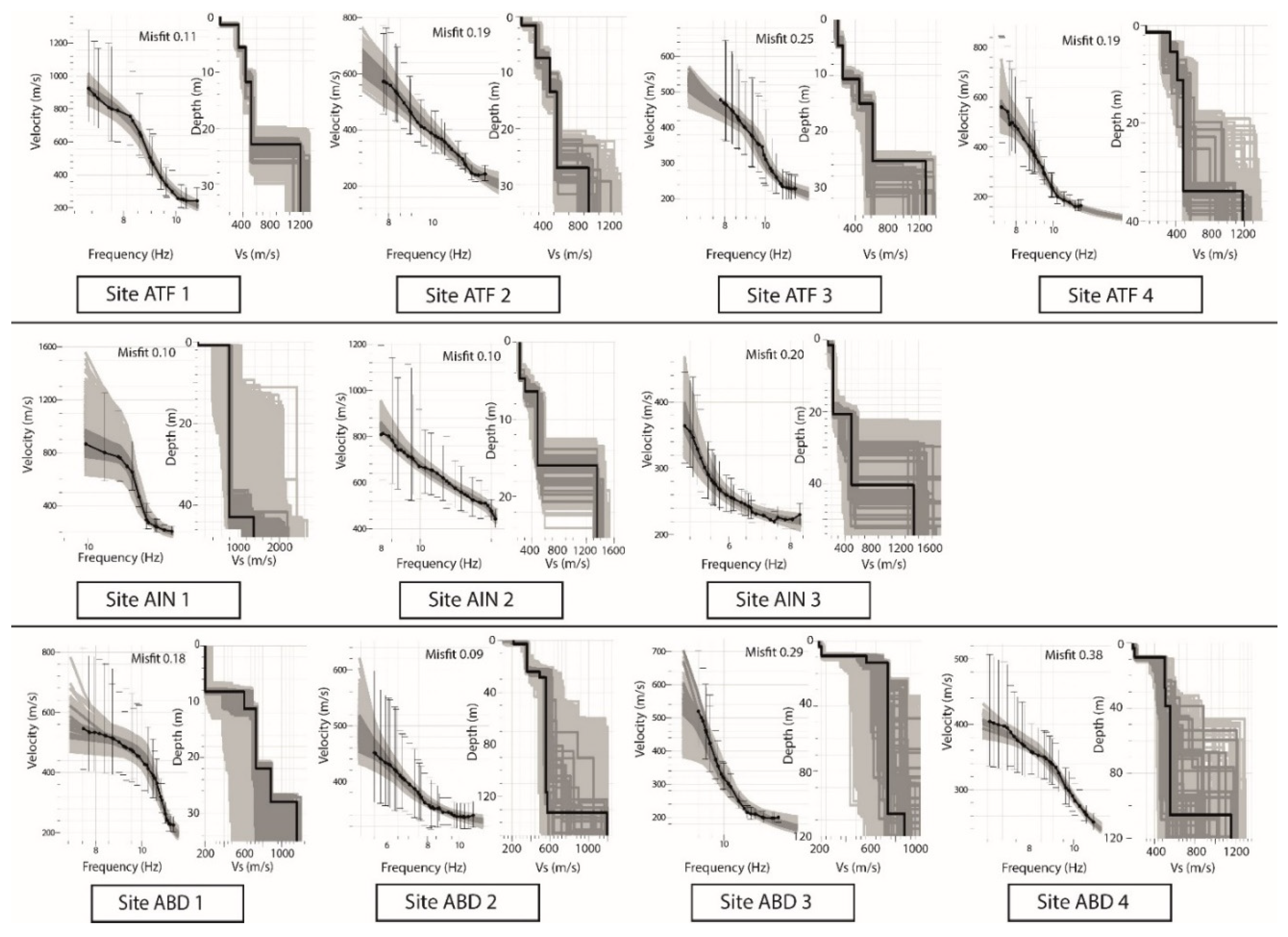
3.4. Inversion of Dispersion Curves and HVSR Curves

The inversion was carried out with the Dinver software (Sesarray package [34]) using the neighborhood algorithm [51]. In order to have a better spatial distribution for the Vs30 values, some HVSR curves were inverted in El-Abadia (5 sites) and Ain-Defla (5 sites). Only the part around the fundamental frequency peak was considered in the inversion process [52]. For the array data inversion process, the 3 dispersion curves obtained for each array using the 3 different techniques (F-K, SPAC, and ESAC) (Figure 4) were averaged to obtain a better constrained dispersion curve with an optimized frequency range. The input parameters required for the inversion (Vp, Vs, densities, and number of layers) were taken from previous studies [14,21]. The maximum number of iterations was set to 300 iterations, and 100 models were generated at each iteration. The experimental average dispersion curve was compared to the theoretical one via a misfit value. Then, the Vs model corresponding to the minimum misfit was selected (Figure 5).

3.5. Estimation of the Vs30

3.5.1. Vs30 from NSPT Measurements

There are a considerable number of studies that propose equations relating shear-wave velocity to the Normalized Standard Penetration Test (NSPT). However, the equations are specific to the region under study. Sil et al. [53] compiled data from different continents and proposed empirical equations correlating NSPT values with shear-wave velocity for sands (Equation (4)), clays (Equation (5)), and for all soil types (Equation (6)):
V S = 79.217 × N 0.3699
V S = 99.708 × N 0.3358
V S = 75.478 × N 0.3799
where VS is the shear-wave velocity and N-value is the number of blows in the SPT measurements. However, in the case the SPT borehole does not reach 30 m, which is the case in this study, V s 30 can be correlated from the average velocity at depth z using the following equation from [54]:
L o g   V s 30 = a + ( b × L o g   V s z )
V s z is the velocity at depth z, and a and b are coefficients that vary with depth (see Table 2 in [54]).

3.5.2. Vs30 from Vs Models

The inversion of the dispersion curves allows retrieval of the Vs models. The averaged V s 30 can be calculated from the Vs models using the following equation [55]:
V s 30 = 30 i = 1 N   H i V i
Hi is the thickness and Vi is the shear-wave velocity of the layer i.
The obtained V s 30 values were then spatially meshed using the Kriging method [56], with a linear transformation. A map of V s 30 variation was obtained for each city. As for the classification of the sites, it was completed according to the NEHRP site classification [57] (Table 2).

4. Results and Discussion

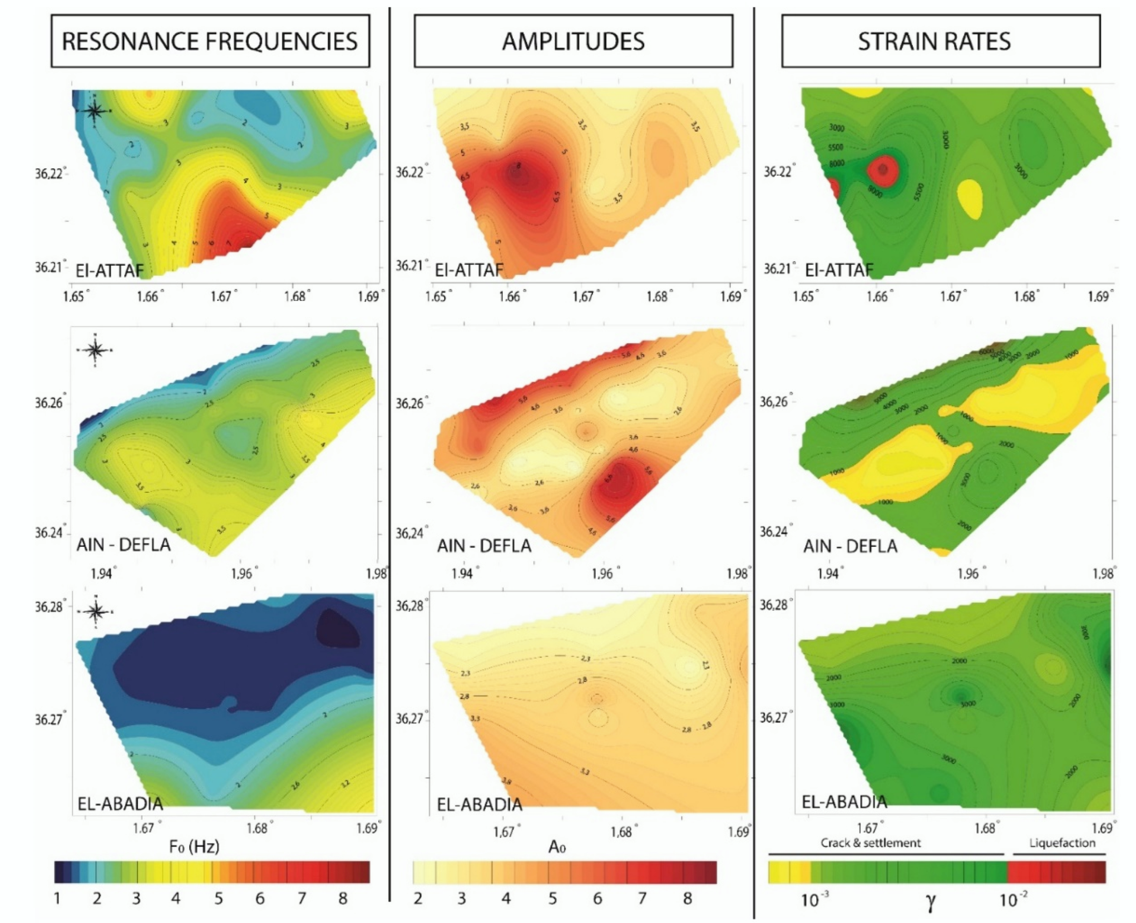
4.1. Soil Resonance Frequencies and Amplitudes

The soil resonance frequencies and the corresponding amplitudes for the cities of El-Attaf, El-Abadia, and Ain-Defla, are mapped in Figure 6. In El-Attaf city, the resonance frequencies are between 1.2 and 8.3 Hz. In the major part of the city, the predominant frequencies are between 1.2 and 5 Hz. The obtained values are related to impedance contrasts in the subsoil between the Quaternary alluviums and the Miocene marls and sandstones. Near Ouled Moussa, south of the city, higher frequencies are observed (between 5 and 8.3 Hz). This increase is most likely related to the Cretaceous marls outcropping in the south [21]. Since the buildings in this area have between 1 and 5 floors, the resonance frequencies of the ground are close to the buildings’ frequencies, which can be damaging for the structures during strong shaking. The predominant amplitudes of the frequency peaks vary between 2.2 and 8.7. The amplitudes are lower to the northern areas of the city. The highest amplitudes (between 5 and 8.7) are observed in “Cité Bouzar” neighborhood, in the western areas of the city.
In the El-Abadia city, the resonance frequencies vary between 1.4 and 4.2 Hz, while the corresponding amplitudes vary between 2 and 4. The obtained resonance frequencies are related to impedance contrasts between the Quaternary alluviums and the Pliocene sandstones. The amplitudes slightly increase to the southwest towards the Middle-Chelif plain, where the Quaternary stiff and soft soils are thicker. Finally, in the Ain-Defla city, the resonance frequencies vary between 1.4 and 4.5. These frequencies are related to the impedance contrasts between the Quaternary deposits and the Cretaceous-Jurassic bedrock. The increase in the resonance frequency peak from north to south is related to the presence of the Doui Massif and its hard Jurassic limestones [22] to the south of the city. The predominant amplitude of the frequency peaks varies between 2 and 7.1. The amplitudes are relatively low in the central part of the city. However, in “Mohamad Khiat” neighborhood, in the SW, the amplitudes are relatively higher (5–7.1). In the northern areas, it reaches a value of 6.8.

4.2. Shear Strain and Liquefaction Potential

The shear strain variation map for the three cities (right column in Figure 6) gives valuable information about the dynamic properties of the soils and the possible behavior during earthquakes. In El-Abadia and Ain-Defla cities, the shear strain values reflect an elasto-plastic soil behavior, where cracks and settlements may occur during strong ground shaking. However, in the central part of Ain-Defla city, the lower strain values indicate that the soil column tends towards a more elastic appearance, which is probably due to the thickening of the ancient Quaternary deposits in this zone, with the presence of very dense clays and gravels [13]. In both cities, the results show that the soils do not show any predisposition to liquefaction and landslide phenomena during earthquakes.
On the other hand, in the El-Attaf city, strain rate shows different dynamic properties of the soil, an elasto-plastic behavior in the east, and a collapse behavior in the west, more precisely in the “Cité Bouzar” neighborhood, with a soil subject to liquefaction. Piezometric measurements in “Cité Bouzar” have shown that the water table is around 7 m deep [15]. The presence of sandbanks and water table at very shallow depths increase the risk of liquefaction in the area, which was the case during the 1980 El-Asnam earthquake. Indeed, liquefaction phenomena were reported west of El-Attaf, where large sand boil formations (>6 m) were observed [9].

4.3. Dispersion Curve Inversion and Vs Models

The dispersion curves obtained using the three techniques, F-K, SPAC, and ESAC, and presented in Figure 4, are plotted within the theoretical limits of the wavenumber (Kmin, Kmax). The dispersion curves are valid between 7 and 12 Hz in El-Attaf and between 5 and 12 Hz in Ain-Defla. In the El-Abadia city, the curves are valid between 5.5 and 11 Hz. This difference is due to local site conditions. The dispersion curves are well correlated at most sites (Figure 4). At sites ATF1 and AIN1, the dispersion curves obtained with the ESAC technique tend to diverge from the other curves at high frequencies. We note that at these sites, the array was deployed on slightly sloping terrain, which might indicate that the ESAC technique could be more sensitive to slopes than the other techniques.
An average curve was calculated at each site. In this way, a better constrained dispersion curve is used for the inversion process to obtain a better consistency of the resulting Vs profiles. The results of the inversion are shown in Figure 5. In the El-Attaf city, the engineering bedrock corresponds to the Miocene marls and sandstones, with a Vs value varying between 970 and 1280 m/s. Soft and stiff Quaternary alluvium occupies the first 30 m of the soil column. In the Ain-Defla city, the bedrock Vs value varies between 1390 and 1450 m/s. The thickness of the Quaternary deposits varies between 16 and 43 m. At El-Abadia city, the bedrock Vs value is divided into two different ranges, between 870 and 900 m/s to the east (ABD1, ABD3), and between 1150 and 1200 m/s to the west (ABD2, ABD4). This difference is related to the change in bedrock composition from Late Pliocene sandstones in the east to Miocene marls and sandstones in the west. The thickness of the Quaternary layers varies between 11 and 29 m.

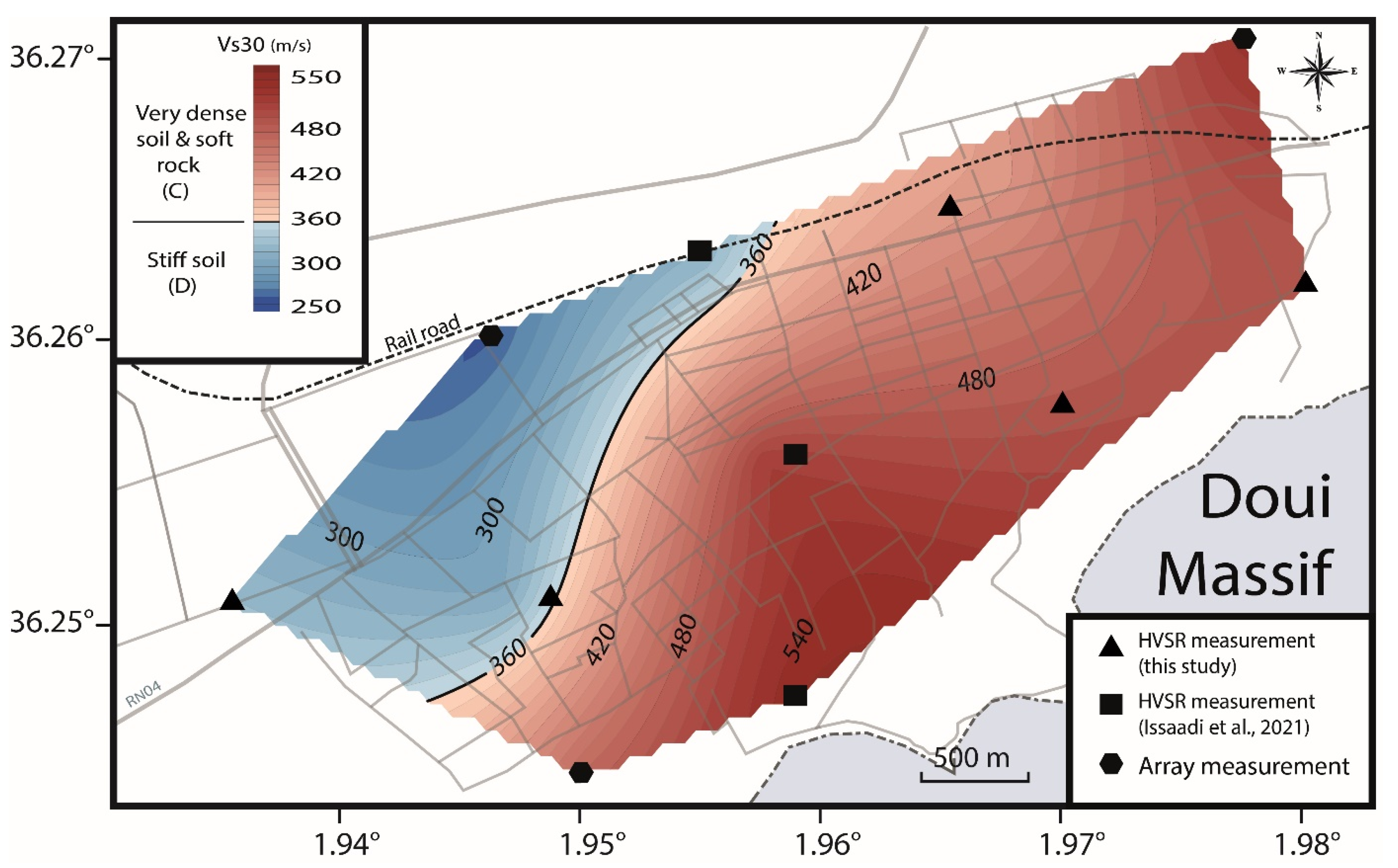
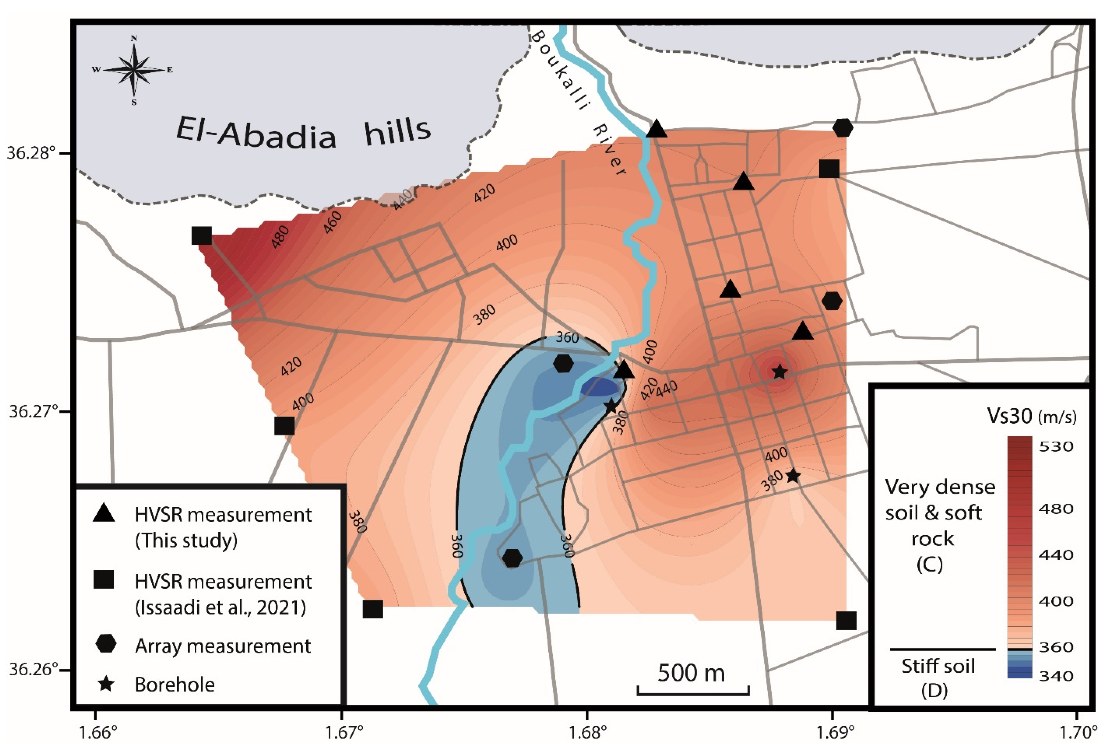
4.4. Vs30 Structure and Site Classification

V s 30 was calculated from the shear-wave velocity models and the additional SPT surveys. A map of V s 30 variation, along with site classification, is provided for each of the three cities (Figure 7, Figure 8 and Figure 9).
In El-Attaf city, the V s 30 values vary between 290 and 460 m/s (Figure 7). In most of the city, the soil is classified as very dense (C), except for a small area in the center where the soil is classified as stiff (D). The increase in velocity towards the west is caused by the presence of shallow Jurassic limestones, which outcrop about 1 km west of the city in the Temoulga Massif (Figure 2). In the southern part of the city, the slight increase in V s 30 is related to the thinning of the Quaternary alluvium and the predominance of the Miocene stiff formations [21].
In the Ain-Defla city, the V s 30 values vary between 250 and 550 m/s (Figure 8). The soil is classified as very dense and soft rock (C) in most of the city. The velocity gradually decreases towards the northwest and the soils become stiff (D). The variation in V s 30 at Ain-Defla is mainly controlled by the ratio of Quaternary alluvium to Jurassic limestone in the first 30 m. In the south, where the city backs onto the Doui Massif, the ancient Quaternary alluvium forms a thin layer and the upper 30 m of the soil is dominated by Jurassic limestone. Moving northwest, the Quaternary deposits begin to be thicker and dominate the top 30 m of the soil column, and thus, V s 30 values decrease and the soils are classified as stiff. In the El-Abadia city, the V s 30 values range from 340 and 530 m/s (Figure 9). In most of the city, soils are classified as very dense and soft rock (C). The high V s 30 values are related to the presence of Pliocene conglomerates and sandstones at shallow depths. The shear-wave velocity values decrease towards the south where the Quaternary alluvium is thicker [16]. The lowest Vs values are observed around the southern part of the Boukalli River in the city, where the upper layer is composed of present alluvium.

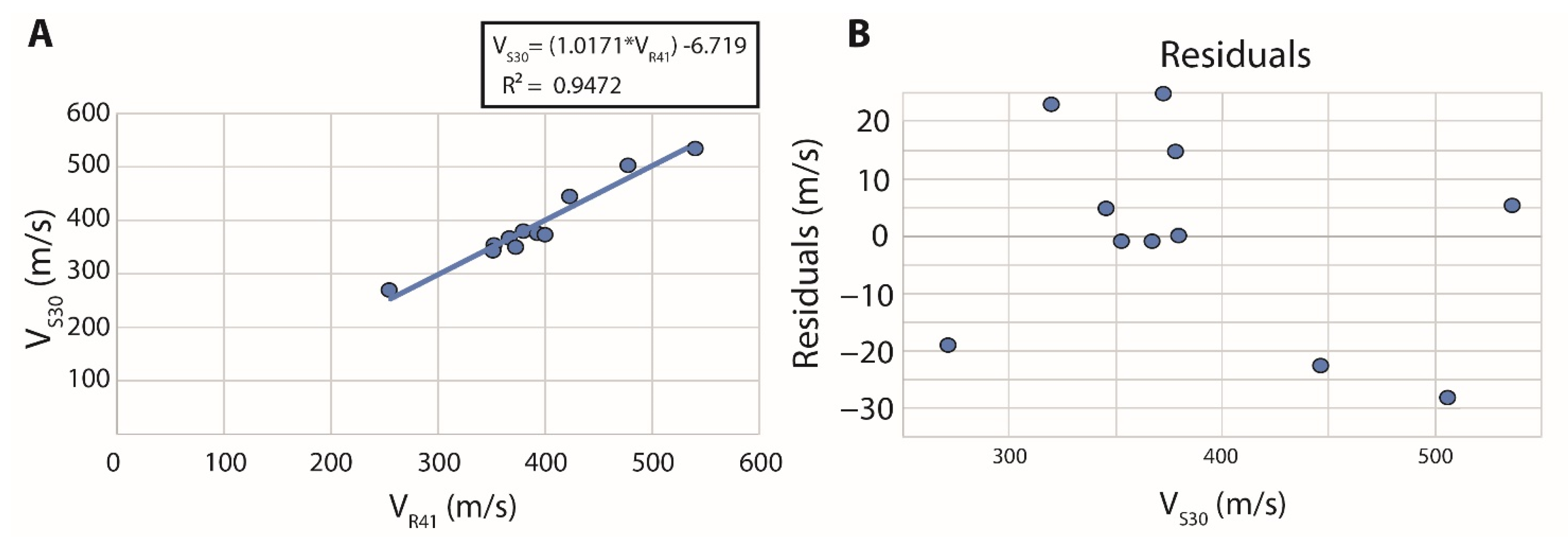
4.5. Vs30 Predictive Equation for the Middle-Chelif Basin

The wavelength corresponding to the V s 30 value was estimated for each average dispersion curve. The average wavelength found is λ = 41 m ± 3. After that, the V s 30 values were correlated with V R 41 values (Rayleigh wave velocity at λ = 41 m), and the best linear fitting was obtained (Equation (9)):
V s 30   =   10171     V R 41 6719
The regression plot, along with the residuals, is shown in Figure 10. The correlation degree is R2 = 0.9472. Equation (9) was applied to dispersion curves obtained in two other cities of the Middle-Chelif Basin from a previous study [21] (Table 3). The aim was to evaluate the reliability of the V s 30 predictive equation. The V s 30 values were predicted within a maximum error of 5.6%, and the site classifications were correct. For the dispersion curves obtained in the present study, the V s 30 values were predicted within a maximum error of 7.6%, and the site classifications were correct, except for ATF1 site.
In the case of the ATF1 site, the estimated and predicted V s 30 values are close to the limit between class C and D (according to the NEHRP classification [57]).

5. Conclusions

In the present study, ambient vibration records were used to characterize the dynamic properties of the soil, and the velocity structure of its upper 30 m ( V s 30 ) in the cities of El-Attaf, Ain-Defla, and El-Abadia, in the Middle-Chelif Basin. Both single-station and array-based techniques were applied. The studied cities are a good example of growing cities located in a highly seismic zone. This study improves the one carried out by the WCC (1984) by investigating the behavior of the soils and quantifying the liquefaction potential. Additionally, the Vs30 values allowed classifying the soils of the three cities for the first time.
The HVSR technique was applied on single-station measurements to estimate the ground resonance frequencies. In the El-Attaf city, the frequencies vary between 1.2 and 8.3 Hz, and between 1.4 and 4.2 Hz in the El-Abadia city. In theAin-Defla city, the resonance frequencies vary between 1.4 and 4.5 Hz. The frequency peaks are directly related to impedance contrasts at different depths between sediments and bedrock. The corresponding amplitudes are ranging between 2 and 8.7.
The obtained resonance frequencies and the corresponding amplitudes were used to calculate the shear strain, which may give an idea about possible behavior of the soils during major earthquakes. In the El-Abadia and Ain-Defla cities, the shear strain values reflect the elasto-plastic behavior of the soil column. Cracks and settlements may occur during earthquakes, especially in El-Abadia city. In El-Attaf, the shear strain analysis also shows an elasto-plastic behavior of the soil in most of the city. Except in its western part, where a collapse behavior is observed. Consequently, the soil is subject to liquefaction.
Rayleigh wave dispersion curves were obtained from array recordings at 11 sites, using F-K, SPAC, and ESAC techniques. Shear-wave velocity models were obtained from the inversion of the mean dispersion curves. From the V s 30 variation maps, the local soils were classified using the NEHRP chart for site classification. In the El-Attaf city, the V s 30 values vary between 300 and 470 m/s. The soil is classified as very dense and soft rock (C) in most of the city. In the Ain-Defla city, V s 30 values vary between 250 and 530 m/s. The soils are classified as very dense (C) in the central and eastern sides. In the west, the soils are stiff (D) due to the thickening of the Quaternary alluviums. Finally, in the El-Abadia city, the V s 30 values vary between 340 and 530 m/s. In the major part of the city, the soil is classified as very dense and soft rock (C). In addition, a predictive equation for V s 30 in the Middle-Chelif Basin was proposed based on the obtained dispersion curves and V s 30 values.
The three studied cities extend to the alluvial plains of the Middle-Chelif, an area of unstable soils, which has undergone several phenomena induced by past earthquakes (e.g., soil liquefaction, landslides, cracks, settlements). A well constrained characterization of the dynamic properties of the soil, as well as the shear-wave velocity structure, allows a better understanding of the soil behavior during strong earthquakes. Therefore, this allows minimizing potential damage during potential earthquakes. The present study aims to contribute to the seismic hazard assessment in northern Algeria.

Author Contributions

A.I. acquired and processed the data and wrote the paper. A.S. acquired and prepared the data, helped with figure conceptualization. F.S. proposed the methodology, the structure, and reviewed the paper. A.Y.-C. provided the acquisition materials and supervised the paper. J.J.G.-M. provided Matlab code and reviewed the paper. All authors have read and agreed to the published version of the manuscript.

Funding

This research received no external funding.

Data Availability Statement

The data used in this study belongs to the research center in astronomy astrophysics and geophysics (CRAAG, Algeria).

Acknowledgments

The authors would like to thank the members of the CRAAG team that participated in field measurements: B. Melouk, O. Haddad, and R. Chimouni.

Conflicts of Interest

The authors declare no conflict of interest.

References

  1. Ayadi, A.; Maouche, S.; Harbi, A.; Meghraoui, M.; Beldjoudi, H.; Mahsas, A.; Benouar, D.; Heddar, A.; Kherroubi, A.; Frogneux, M.; et al. Strong Algerian earthquake strikes near Capital city. EOS 2003, 84, 561–568. [Google Scholar] [CrossRef]
  2. Abacha, I.; Boulahia, O.; Yelles-Chaouche, A.; Semmane, F.; Beldjoudi, H.; Bendjama, H. The 2010 Beni-Ilmane, Algeria, earthquake sequence: Statistical analysis, source parameters, and scaling relationships. J. Seismol. 2019, 23, 181–193. [Google Scholar] [CrossRef]
  3. Ait Benamar, D.; Moulouel, H.; Belhai, D.; Semmane, F.; Harbi, A.; Tebbouche, M.Y.; Boukri, M.; Meziani, A.A.; Aourari, S.; Braham, M. The 17 July 2013 Hammam Melouane earthquake: Observations and analysis of geological and seismological data. J. Iber. Geol. 2022, 48, 163–180. [Google Scholar] [CrossRef]
  4. Yelles-Chaouche, A.; Boudiaf, A.; Djellit, H.; Bracene, R. La tectonique active de la région nord-algérienne. Comptes Rendus Geosci. 2006, 338, 126–139. [Google Scholar] [CrossRef]
  5. Meghraoui, M. Géologie des Zones Sismiques du Nord de l'Algérie: Paléosismologie, Tectonique Active et Synthèse Sismotectonique. Ph.D. Thesis, Université de Paris-Sud, Paris, France, 1988. [Google Scholar]
  6. Ouyed, M.; Meghraoui, M.; Cisternas, A.; Deschamps, A.; Dorel, J.; Frechet, J.; Gaulon, R.; Hatzfeld, D.; Philip, H. Seismotectonics of the El Asnam earthquake. Nature 1981, 292, 26–31. [Google Scholar] [CrossRef]
  7. Benouar, D. Materials for the Investigation of the Seismicity of Algeria and Adjacent Regions during the Twentieth Century; Annali Di Geofisica: Roma, Italia, 1994; pp. 459–860. [Google Scholar]
  8. Philip, H.; Meghraoui, M. Structural analysis and interpretation of the surface deformations of the El Asnam earthquake of October 10, 1980. Tectonics 1983, 2, 17–49. [Google Scholar] [CrossRef]
  9. Clough, W.G.; Mass, S.S.; Hamou, A.h. Observation of Liquefaction and Landsliding as a Result of the October 10, 1980 El-Asnam, Algeria Earthquake; Blume Earthquake Engineering Center, Departement of Civil Engineering, Stanford University: Stanford, CA, USA, 1981; p. 43. [Google Scholar]
  10. Perrodon, A. Etude géologique des bassins sublittoraux de l'Algérie occidentale. Publ. Serv. Cart. Géologique L’Algérie 1957, 12, 328. [Google Scholar]
  11. Repal, S.N. Le basin néogène du Chélif. In Proceedings of the XIXe Congrés de Géologie International, Alger, Algeria, 1952; p. 56. Available online: https://www.abebooks.fr/rechercher-livre/titre/le-bassin-neogene-du-chelif/auteur/repal-s-n/ (accessed on 27 June 2022).
  12. Brives, A. Les Terrains Miocenes du Bassin du Chélif et du Dahra; Imprimerie P. Fontana & Cie: Algiers, Algeria, 1897. [Google Scholar]
  13. CGG. Geophysical Study of the Cheliff Plain; Internal report; Compagnie Generale de Geophysique: Paris, France, 1969. [Google Scholar]
  14. Talaganov, K.; Aleksovski, D.; Milutinovic, Z.; Ameur, B.; Arsovski, M.; Jancevski, J.; Andreevski, V. Studies for Elaboration of the Code for Repair and Strengthening of Damaged Buildings in the Region of El Asnam: Engineering Geology, Geotechnical and Geophysical Characteristics of the TOWN of El Asnam and Other Sites; Report IZIIS; Institute of Earthquake Engineering & Engineering Seismology: Skopje, North Macedonia, 1982; pp. 55–82. [Google Scholar]
  15. Woodward-Clyde Consultants. Seismic Microzonation of Ech-Chellif Region, Algeria; Woodward-Clyde Consultants: London, UK, 1984. [Google Scholar]
  16. Meghraoui, M. Etude neotectonique de la region nord-est d’El Asnam: Relation avec le seisme du 10.10. 1980. Ph.D. Thesis, Université de Paris VII, Paris, France, 1982. [Google Scholar]
  17. Bendali, M.; Abtout, A.; Bouyahiaoui, B.; Boukerbout, H.; Marok, A.; Reolid, M. Interpretation of new gravity survey in the seismogenic Upper Chelif Basin (North of Algeria): Deep structure and modeling. J. Iber. Geol. 2022, 48, 205–224. [Google Scholar] [CrossRef]
  18. Layadi, K.; Semmane, F.; Yelles-Chaouche, A. Site-Effects Investigation in the City of Chlef (Formerly El-Asnam), Algeria, Using Earthquake and Ambient Vibration Data. Bull. Seismol. Soc. Am. 2016, 106, 2185–2196. [Google Scholar] [CrossRef]
  19. Layadi, K.; Semmane, F.; Yelles-Chaouche, A. S-wave velocity structure of Chlef City, Algeria, by inversion of Rayleigh wave ellipticity. Near Surf. Geophys. 2018, 16, 328–339. [Google Scholar] [CrossRef]
  20. Issaadi, A.; Semmane, F.; Yelles-Chaouche, A.; Galiana-Merino, J.; Layadi, K. A Shear-Wave Velocity Model in the City of Oued-Fodda (Northern Algeria) from Rayleigh Wave Ellipticity Inversion. Appl. Sci. 2020, 10, 1717. [Google Scholar] [CrossRef]
  21. Issaadi, A.; Semmane, F.; Yelles-Chaouche, A.; Galiana-Merino, J.J.; Mazari, A. Shallow S-wave velocity structure in the Middle-Chelif Basin, Algeria, using ambient vibration single-station and array measurements. Appl. Sci. 2021, 11, 11058. [Google Scholar] [CrossRef]
  22. Kireche, O. Etude Géologique et Structurale des Massifs de la Plaine du Chéliff (Doui, Rouina, Temoulga). Ph.D. Thesis, Université d’Alger, Algiers, Algeria, 1977. [Google Scholar]
  23. Thomas, G. Géodynamique d’un Bassin Intramontagneux: Le Bassin du bas Chéliff Occidental (Algérie) durant le Mio-Plio-Quaternaire. Ph.D. Thesis, Université de Pau, Pau, France, 1985. [Google Scholar]
  24. Brives, A.; Jackob, M.; Ficheur, M. Carte Géologique de Oued-Fodda 1/50.000; Service Géologique de l’Algérie: Algiers, Algeria, 1906. [Google Scholar]
  25. Nakamura, Y. A method for dynamic characteristics estimation of subsurface using microtremor on the ground surface. Railw. Tech. Res. Inst. Q. Rep. 1989, 30, 25–33. [Google Scholar]
  26. Field, E.H.; Jackob, K.H. A comparison and test of various site response estimation techniques, including three that are non reference—Site dependent. Bull. Seismol. Soc. Am. 1995, 85, 1127–1143. [Google Scholar]
  27. Arai, H.; Tokimasu, K. S-wave velocity profiling by inversion of microtremor H/V spectrum. Bull. Seismol. Soc. Am. 2004, 94, 53–63. [Google Scholar] [CrossRef]
  28. Bonnefoy-Claudet, S.; Cornou, C.; Bard, P.Y.; Cotton, F.; Moczo, P.; Kristek, J.; Fäh, D. H/V ratio: A tool for site effects evaluation: Results from 1D noise simulations. J. Appl. Geophys. 2006, 167, 827–837. [Google Scholar] [CrossRef]
  29. Rosa-Cintas, S.; Galiana-Merino, J.; Rosa-Herranz, J.; Molina, S.; Martínez-Esplá, J. Polarization analysis in the stationary wavelet packet domain: Application to HVSR method. Soil Dyn. Earthq. Eng. 2012, 42, 246–254. [Google Scholar] [CrossRef]
  30. Bonnefoy-Claudet, S.; Cotton, F.; Bard, P.-Y. The nature of noise wavefield and its applications for site effects studies: A literature review. Earth-Sci. Rev. 2006, 79, 205–227. [Google Scholar] [CrossRef]
  31. La Rocca, M.; Chiappetta, G.; Gervasi, A.; Festa, R.L. Non-Stability of the noise HVSR at sites near or on topographic heights. Geophys. J. Int. 2020, 222, 2162–2171. [Google Scholar] [CrossRef]
  32. Benkaci, N.; El Hadi Oubaiche, J.-L.C.; Bensalem, R.; Benouar, D.; Abbes, K. Non-Stability and Non-Reproducibility of Ambient Vibration HVSR Peaks in Algiers (Algeria). J. Earthq. Eng. 2021, 25, 853–871. [Google Scholar] [CrossRef]
  33. Acerra, C.; Aguacil, G.; Anastasiadis, A.; Atakan, K.; Azzara, R.; Bard, P.-Y.; Basili, R.; Bertrand, E.; Bettig, B.; Blarel, F. Guidelines for the Implementation of the H/V Spectral Ratio Technique on Ambient Vibrations Measurements, Processing and Interpretation; European Commission: Louxembourg, 2004. [Google Scholar]
  34. Wathelet, M.; Chatelain, J.L.; Cornou, C.; Giulio, G.D.; Guillier, B.; Ohrnberger, M.; Savvaidis, A. Geopsy: A user-friendly open-source tool set for ambient vibration processing. Seismol. Res. Lett. 2020, 91, 1878–1889. [Google Scholar] [CrossRef]
  35. Konno, K.; Ohmachi, T. Ground-motion characteristics estimated from spectral ratio between horizontal and vertical components of microtremor. Bull. Seismol. Soc. Am. 1998, 88, 228–241. [Google Scholar] [CrossRef]
  36. Ishihara, K. Soil Behaviour in Earthquake Geotechnics; Oxford University Press: Oxford, UK, 1996. [Google Scholar]
  37. Nakamura, Y. Seismic vulnerability indices for ground and structures using microtremor. In Proceedings of the World Congress on Railway Research in Florence, Florence, Italy, 16–19 November 1997. [Google Scholar]
  38. Regles Parasismiques Algerienne RPA99/Version 2003; RPA99/2003. Centre National de Recherche Appliquée en Génie Parasismique: Algiers, Algeria, 2003.
  39. Kelly, E.J.; Levin, M.J. Signal Parameter Estimation for Seismometer Arrays; Massachusetts Institute of Technologies, Lincoln Lab Lexington: Cambridge, MA, USA, 1964. [Google Scholar]
  40. Capon, J.; Greenfield, R.; Kolker, R. Multidimensional maximum-likelihood processing of a large aperture seismic array. Proc. IEEE 1967, 55, 192–211. [Google Scholar] [CrossRef]
  41. Capon, J. High-resolution frequency–wavenumber spectral analysis. Proc. IEEE 1969, 57, 1408–1419. [Google Scholar] [CrossRef]
  42. Lacoss, R.T.; Kelly, E.J.; Toksoz, M.N. Estimation of seismic noise structure using Array. Geophysics 1969, 29, 21–38. [Google Scholar] [CrossRef]
  43. Aki, K. Space and time spectra of stationary stochastic waves, with special reference to microtremors. Bull. Earthq. Res. Inst. 1957, 35, 415–456. [Google Scholar]
  44. Okada, H. The Microtremor Survey Method Geophysical Monograph Series 12; Asten, M.W., Ed.; Society of Exploration Geophysicists: Tulsa, OK, USA, 2003. [Google Scholar]
  45. Bettig, B.; Bard, P.; Scherbaum, F.; Riepl, J.; Cotton, F.; Cornou, C.; Hatzfeld, D. Analysis of dense array noise measurements using the modified spatial auto-correlation method (SPAC): Application to the Grenoble area. Boll. Geofis. Teor. Ed Appl. 2001, 42, 281–304. [Google Scholar]
  46. Ling, S. An extended use of the spatial autocorrelation method for the estimation of geological structure using microtremors. In Proceedings of the 89th SEGJ (The Society Exploration Geophysicists of Japan) Conference, Nagoya, Japan, 12–14 October 1993; pp. 44–48. [Google Scholar]
  47. Parolai, S.; Mucciarelli, M.; Gallipoli, M.R.; Richwalski, S.M.; Strollo, A. Comparison of empirical and numerical site responses at the Tito Test Site, Southern Italy. Bull. Seismol. Soc. Am. 2007, 97, 1413–1431. [Google Scholar] [CrossRef]
  48. Rost, S. Array Seismology: Methods and Applications. Rev. Geophys. 2002, 40, 2-1–2-27. [Google Scholar] [CrossRef]
  49. Köhler, A.; Ohrnberger, M.; Scherbaum, F.; Wathelet, M.; Cornou, C. Assessing the reliability of the modified three-component spatial autocorrelation technique. Geophys. J. Int. 2007, 168, 779–796. [Google Scholar] [CrossRef]
  50. Galiana-Merino, J.J.; Rosa-Cintas, S.; Rosa-Herranz, J.; Garrido, J.; Peláez, J.A.; Martino, S.; Delgado, J. Array measurements adapted to the number of available sensors: Theoretical and practical approach for ESAC method. J. Appl. Geophys. 2016, 128, 68–78. [Google Scholar] [CrossRef]
  51. Wathelet, M. An improved neighborhood algorithm: Parameter conditions and dynamic scaling. Geophys. Res. Lett. 2008, 35, 5. [Google Scholar] [CrossRef]
  52. Fäh, D.; Kind, F.; Giardini, D. Inversion of local S-wave velocity structures from average H/V ratios, and their use for the estimation of site-effects. J. Seismol. 2003, 7, 449–467. [Google Scholar] [CrossRef]
  53. Sil, A.; Haloi, J. Empirical correlations with standard penetration test (SPT)-N for estimating shear wave velocity applicable to any region. Int. J. Geosynth. Ground Eng. 2017, 3, 22. [Google Scholar] [CrossRef]
  54. Boore, D.M. Estimating Vs30(or NEHRP site classes) from shallow velocity models (depths < 30 m). Bull. Seismol. Soc. Am. 2004, 94, 591–597. [Google Scholar]
  55. Code, P. Eurocode 8: Design of Structures for Earthquake Resistance-Part 1: General Rules, Seismic Actions and Rules for Buildings; European Committee for Standardization: Brussels, Belgium, 2005. [Google Scholar]
  56. Cressie, N. The origins of kriging. Math. Geol. 1990, 22, 239–252. [Google Scholar] [CrossRef]
  57. BSS Council. NEHRP Recommended Provisions for Seismic Regulations for New Buildings and Other Structures (FEMA 450); Federal Emergency Management Agency: Washington, DC, USA, 2003. [Google Scholar]
Figure 1. Location of the study area. The numbered yellow stars correspond to the epicenters of the major earthquakes in the area: (1) the 1934 Carnot (I0 = IX) earthquake, (2) the 1954 Orléansville (Ms 6.7) earthquake, and (3) the 1980 El-Asnam earthquake (Mw 7.2). EAF = El-Asnam fault trace; UCB = Upper-Chelif Basin; MCB = Middle-Chelif Basin; LCB = Lower-Chelif Basin.
Applsci 12 08069 g001
Figure 2. Geological map of the study area. Compiled and modified from [22,24].
Applsci 12 08069 g002
Figure 3. Distribution of the data compiled in this study. The orange circles correspond to data measured in [21]. The left panels correspond to the legend, the borehole data, and the array configuration, from top to bottom, respectively. Bh03 was taken from [14]. The rest was taken from [15].
Applsci 12 08069 g003
Figure 4. Rayleigh wave dispersion curves obtained from the F-K, SPAC, and ESAC methods.
Applsci 12 08069 g004
Figure 5. Results of the inversion of Rayleigh waves dispersion curves. The left panels for each site represent the dispersion curves. The right panels represent the Vs models. The black line corresponds to the best fit model, the dark grey represents models with minimum misfit + 10%. All the tested models are in light grey. The misfit is shown at the middle top of each site.
Applsci 12 08069 g005
Figure 6. Results of the single−station measurements analysis.
Applsci 12 08069 g006
Figure 7. V s 30 map and soil classification in the El-Attaf city [21].
Applsci 12 08069 g007
Figure 8. V s 30 map and soil classification in the Ain-Defla city [21].
Applsci 12 08069 g008
Figure 9. V s 30 map and soil classification in the El-Abadia city [21].
Applsci 12 08069 g009
Figure 10. (A) Regression line (VS30 vs. VR41) and equation given. R2 is the correlation coefficient. (B) The corresponding residual values.
Applsci 12 08069 g010
Table 1. Strain dependence of dynamic properties of the soil [36].
Size of Strain Υ10−610−410−310−210−1
PhenomenaWaveVibrationCrackSettlementLandslide, soil compaction, liquefaction
Dynamic propertiesElasticityElasto-plasticityCollapse
Table 2. NEHRP soil classification as a function of the average shear-wave velocity to 30 m depth [57].
Title 1Title 2Title 3
Vs > 1500.Hard rockA
760 < Vs ≤ 1500RockB
360 < Vs ≤ 760Very dense soil and soft rockC
180 < Vs ≤ 360Stiff soilD
Vs ≤ 180Soft soilE
Table 3. Evaluation of V s 30 predictive equation based on Vs30 values obtained in this study, and in [21].
SiteLocation.Vs30 (m/s)Predicted Vs30 (m/s)Error (%)Actual Site ClassificationPredicted Site Classification
This study
ATF1EL-Attaf349.85371.645.9DC
ATF2EL-Attaf373.97399.106.3CC
ATF3EL-Attaf379.08379.270.0CC
ATF4EL-Attaf367.03366.050.3CC
AIN1Ain-Defla505.73477.426.0CC
AIN2Ain-Defla535.85541.501.0CC
AIN3Ain-Defla270.42251.427.6DD
ABD1El-Abadia445.84423.005.4CC
ABD2El-Abadia352.64351.300.4DD
ABD3El-Abadia377.57392.493.8CC
ABD4El-Abadia345.05349.981.4DD
Ref. [21]
AR1Oued-Fodda225.87230.852.2DD
AR2Oued-Fodda223.65211.805.6DD
AR3Oued-Fodda449.07457.901.9CC
AR4Oued-Fodda402.88412.222.3CC
AR5Oued-Fodda467.75457.902.2CC
AR7El-Amra454.45469.593.2CC
Publisher’s Note: MDPI stays neutral with regard to jurisdictional claims in published maps and institutional affiliations.

