
Electricity Price Instability over Time: Time Series Analysis and Forecasting

 ,
,  ,
,  and
and
Abstract
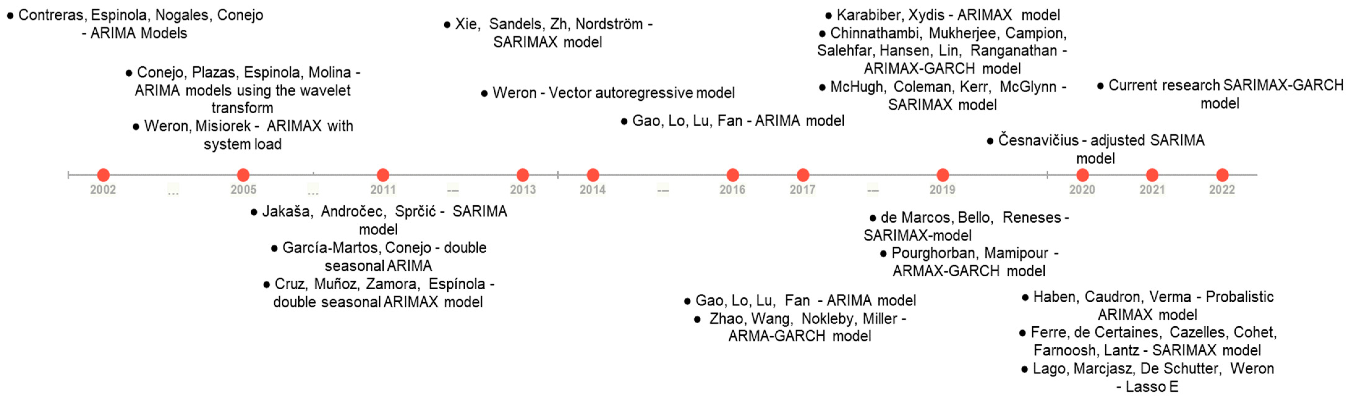
:1. Introduction
2. Materials and Methods
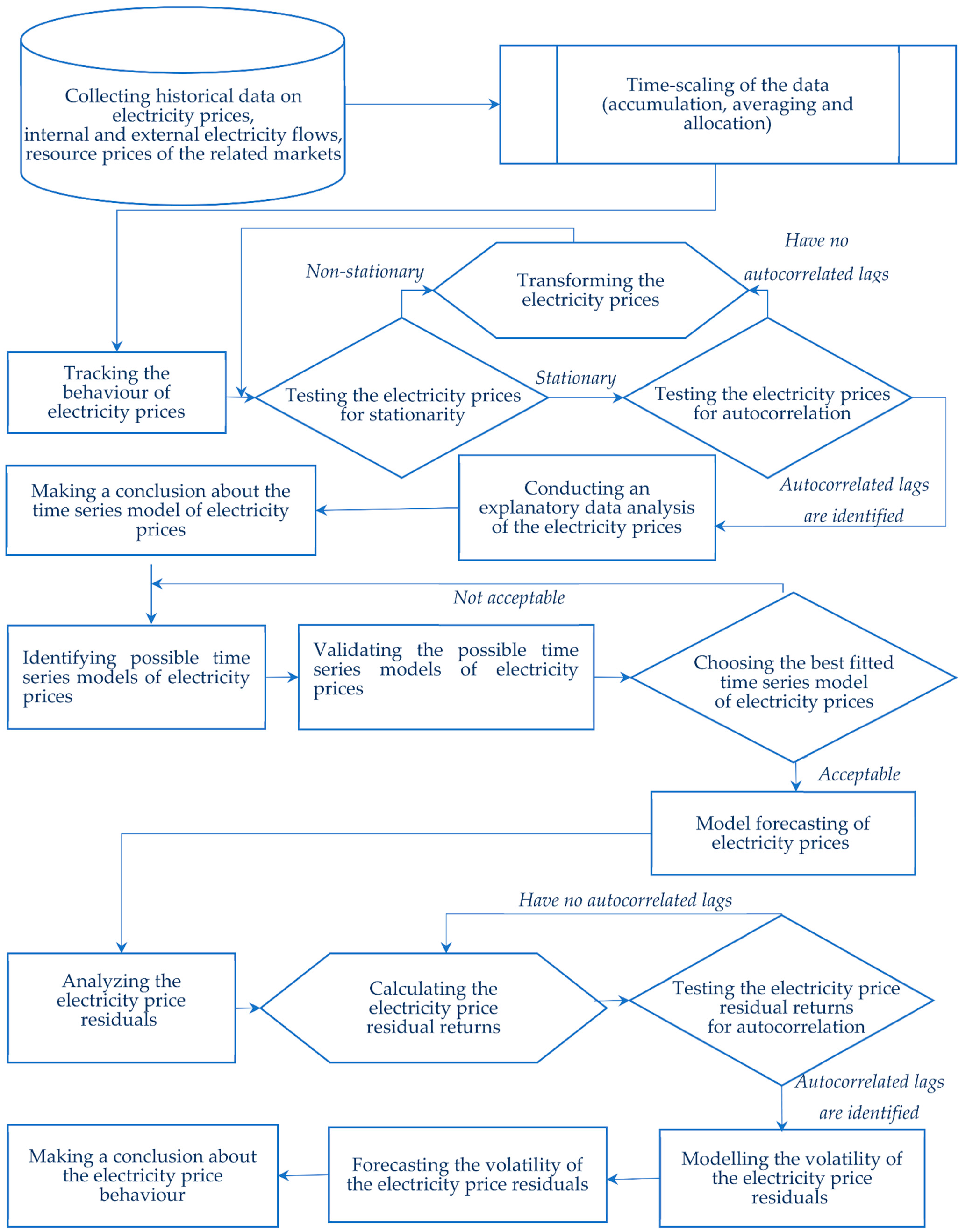
2.1. Methodological Approach
2.2. Data Collection and Preparation
2.3. Data Analysis
2.4. Model Development and Forecasting
- (1)
- (2)
- (3)
- (4)
- SARIMAX (p, d, q) (P, D, Q, s)×, developed by Holst et al. (1988) [52]:where p is the autoregressive component; q is the moving average component; d is the integration order (the number of times needed to ensure stationarity); P is the seasonal variation of the autoregressive component; Q is the seasonal variation of the moving average component; D is the seasonal integration order; s is the length of the seasonal cycle; Yt, Yt−i are the values in the current period and i periods ago, respectively; ∆d is the difference between the values in the current period and d periods ago; are error terms for the current period and j periods ago; c is the baseline constant factor; is the part of the value i periods ago relevant in explaining the current one; is the seasonal lagged value s × l periods ago; is the seasonal lagged error for s × k periods ago; is the part of the error for j periods ago relevant in explaining the current value; is the part of the seasonal lagged value l periods ago relevant in explaining the current one; is the part of the seasonal lagged error for k periods ago relevant in explaining the current value; X is the exogeneous factor; is the slope coefficient for the exogeneous factor.
3. Results
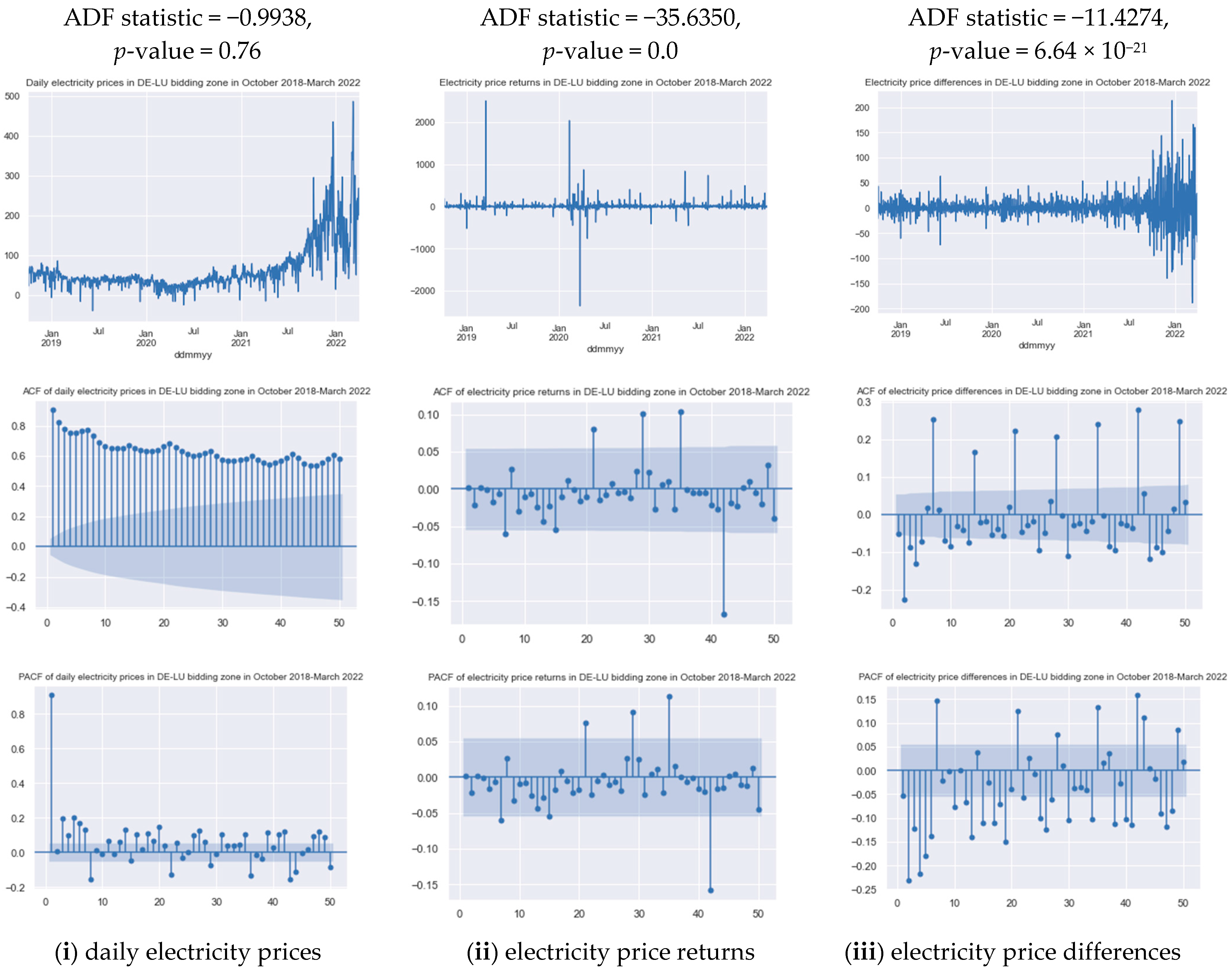
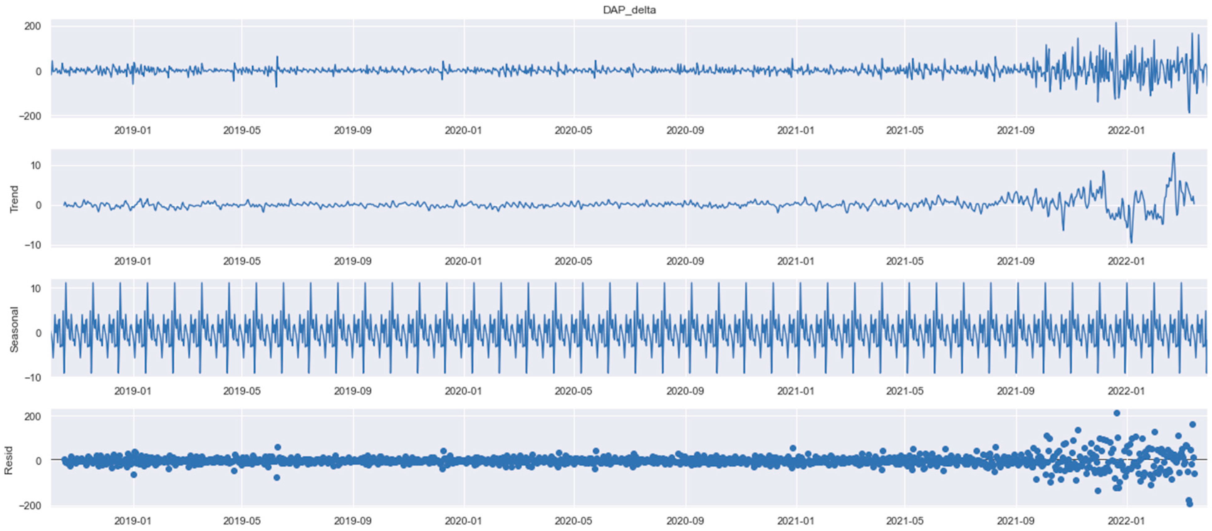
3.1. Data Analysis of Electricity Prices
- The time series of the daily electricity prices are non-stationary. Thus, the null hypothesis has failed to be rejected. The electricity prices have a partly time-dependent structure with no constant variance over time. In this regard, they cannot be used as raw data for the analysis and forecasting;
- Whereas the time series of electricity price returns and electricity price differences are stationary, their current values are conditional and can be used for forecasting,the ACF and PACF plots for electricity price returns show no significant lags, i.e., immediate and secondary impacts of the past values of the time series on the current periods;
- The ACF and PACF plots for electricity price differences show numerous impacts, which proves the expediency of using the ARIMA model based on exact difference–stationary time series;
- The ACF plot of electricity price differences also indicates the presence of seasonality every 7 lags, which corresponds to a weekly cycle of electricity consumption and, accordingly, fluctuations in the electricity prices.
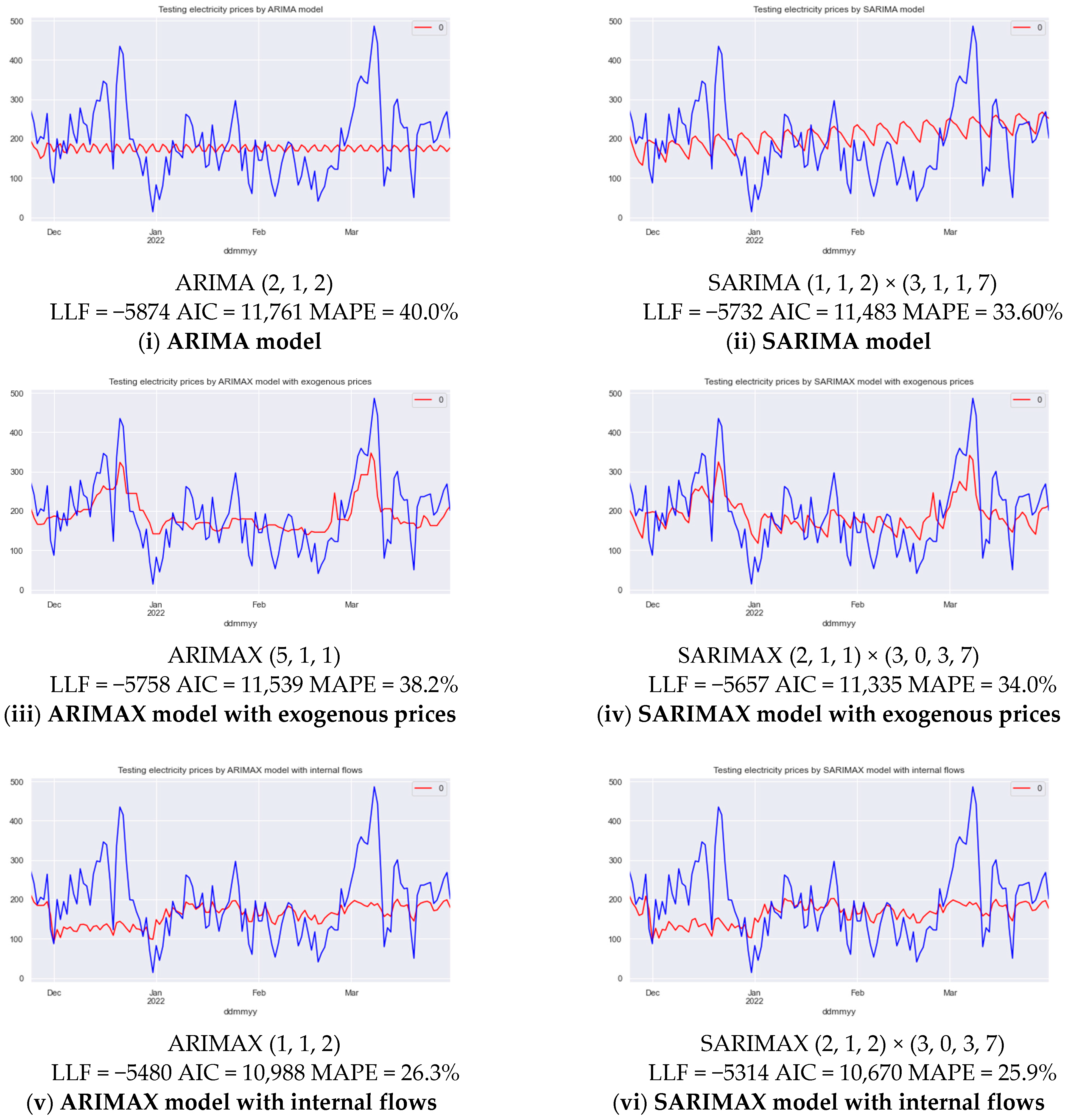
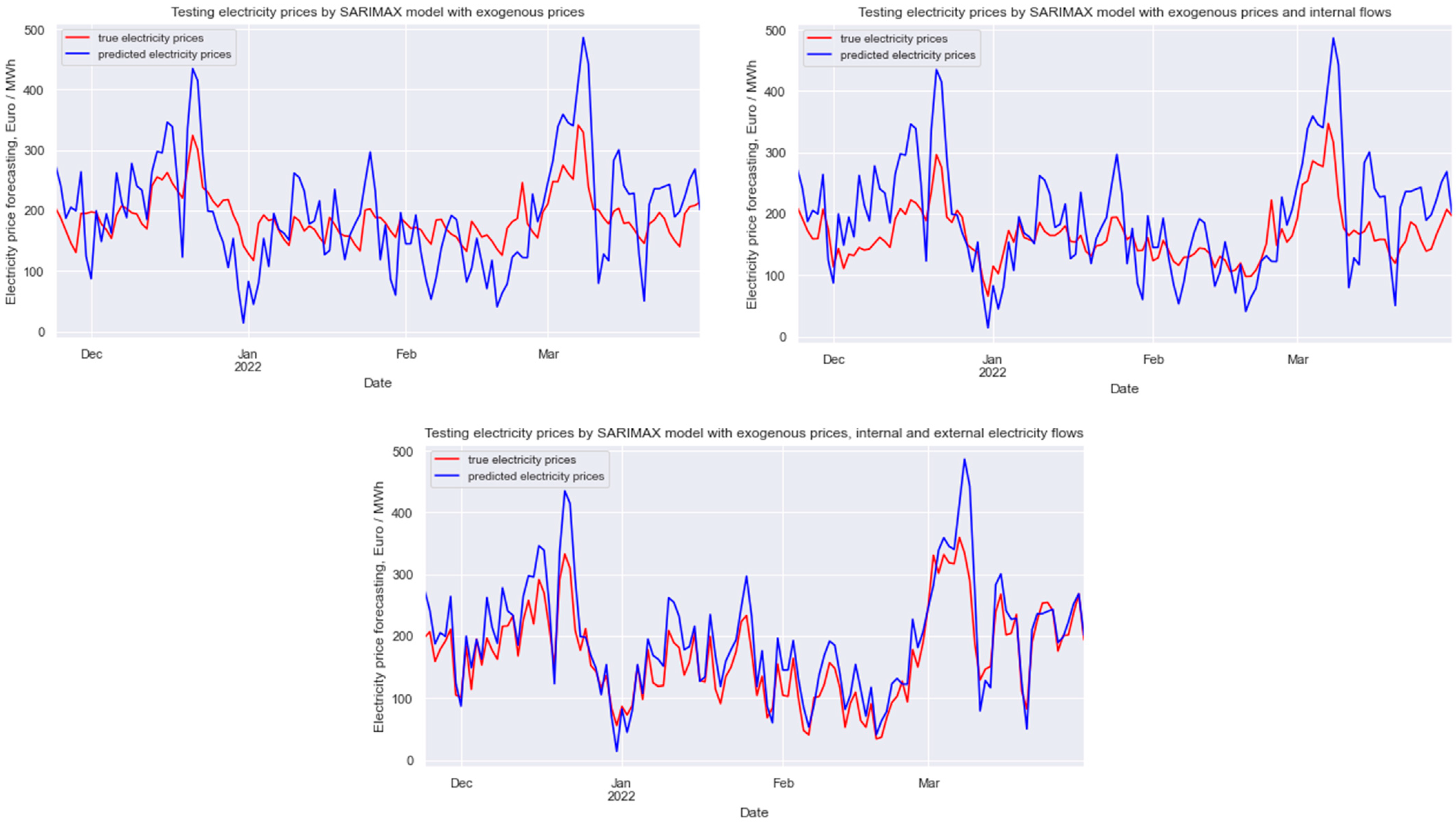
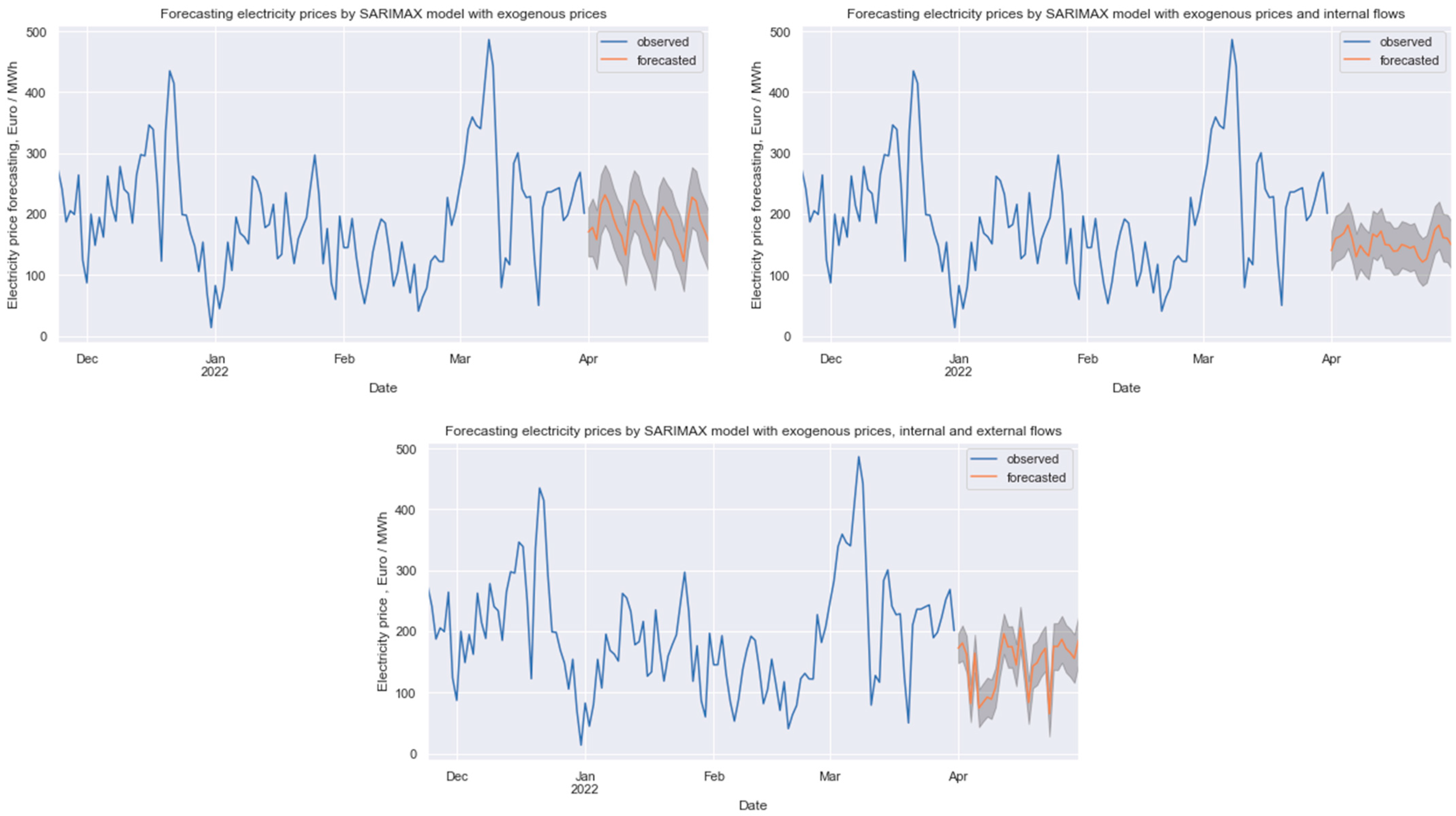
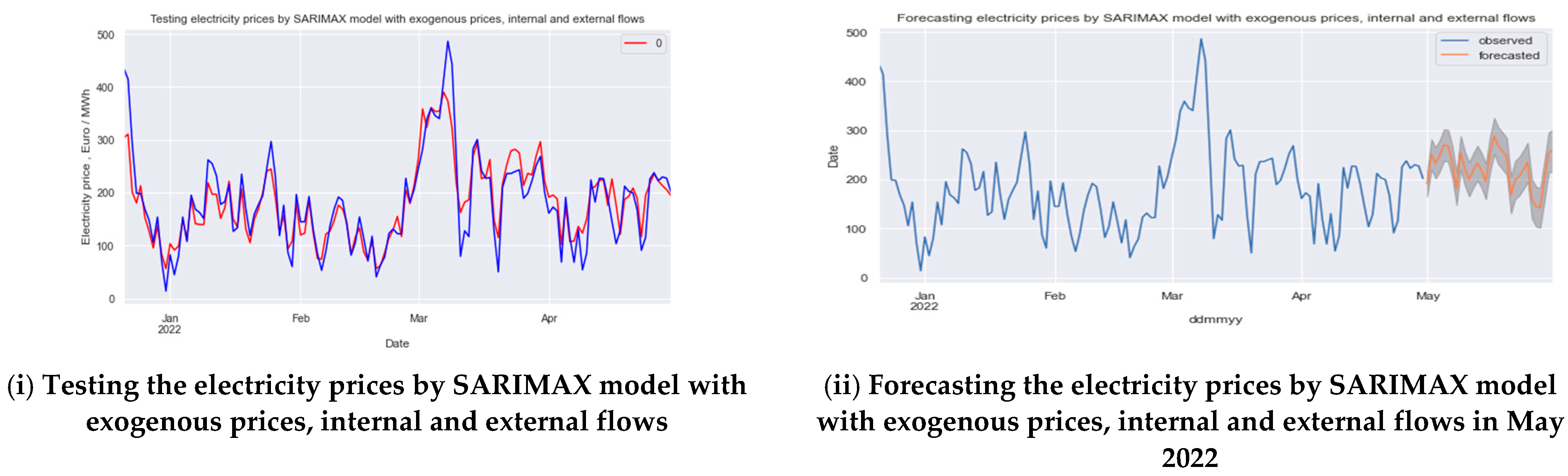
3.2. Time Series Analysis of Electricity Prices and Their Forecasting
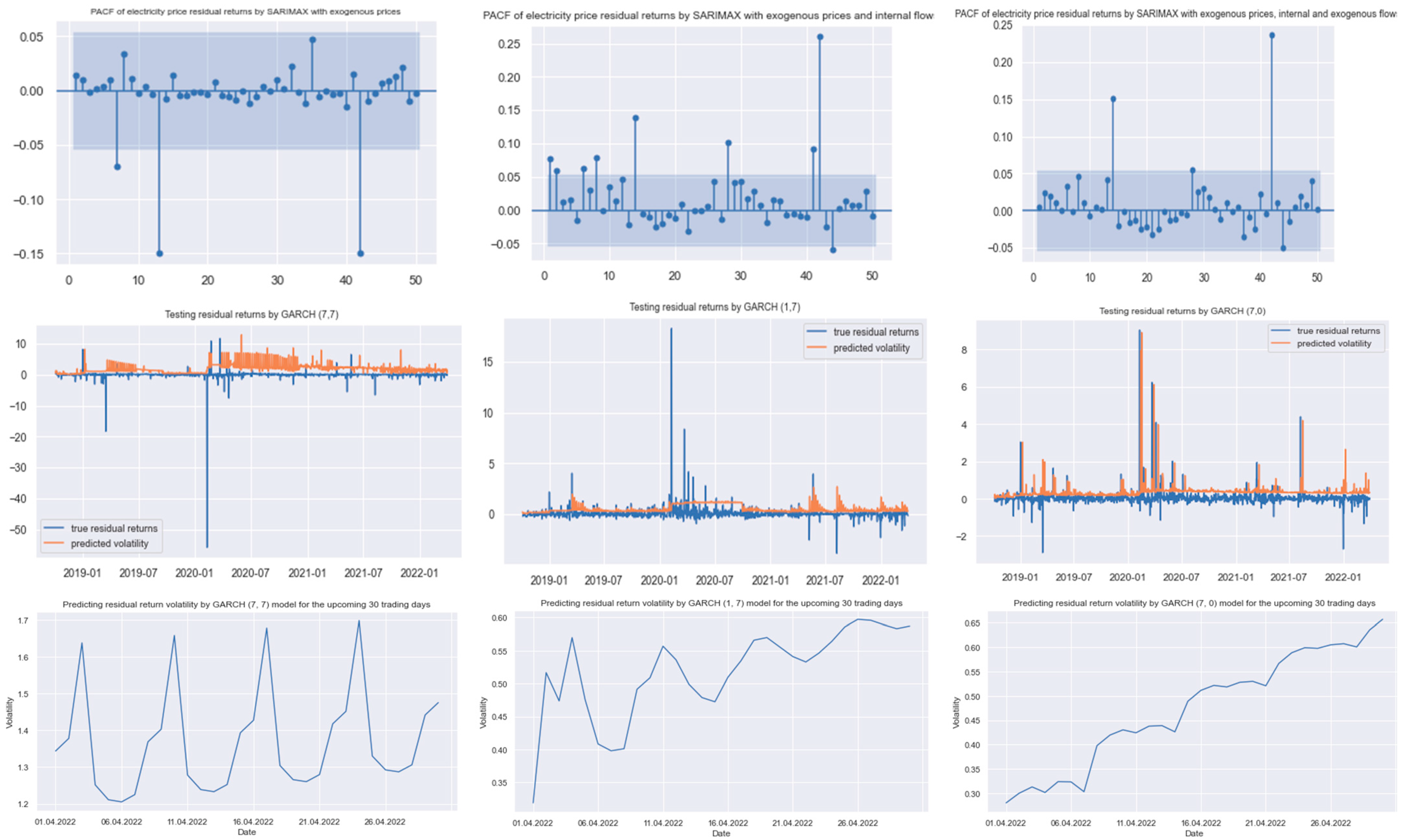
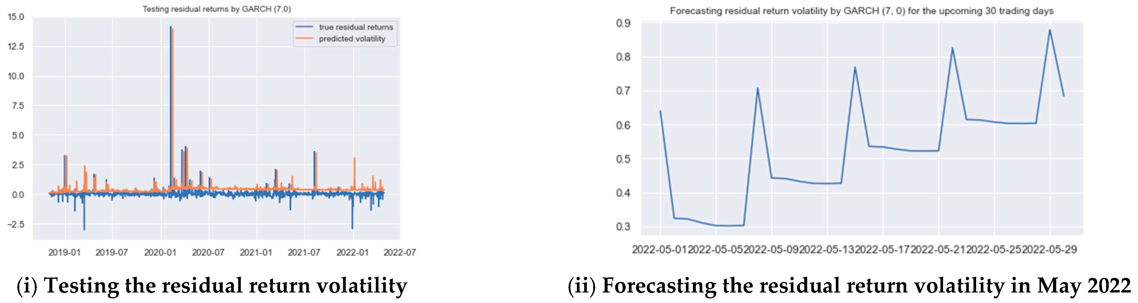
3.3. Residual Forecasting
4. Discussion and Conclusions
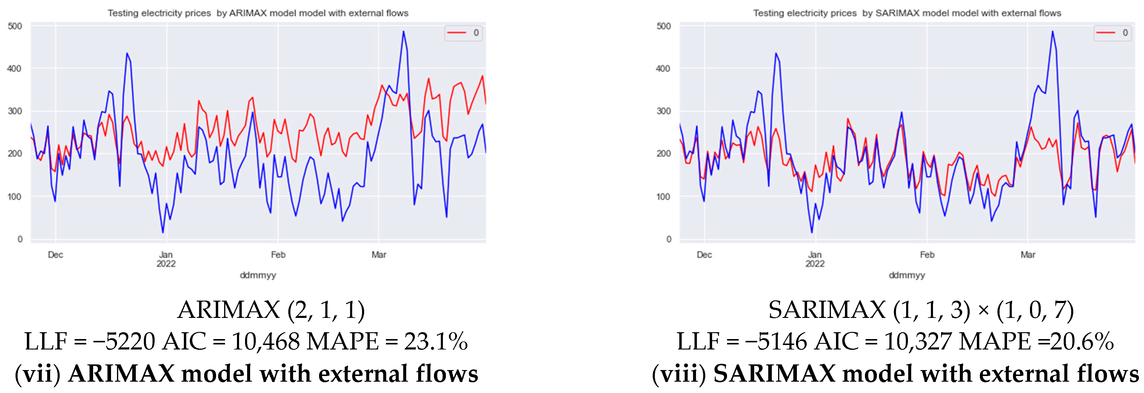
- SARIMAX modelling of the influence of fundamental factors of the internal and external related markets on the changes in electricity prices over time. These factors are considered to be: (i) exogenous prices (gas, coal and CO2 prices), (ii) internal (consumption and generation) electricity flows, and (iii) external (net import) electricity flows;
- GARCH modelling of the volatility of the electricity price residuals, which allows tracking and forecasting the risks of price distortions under the influence of individual trading strategies of electricity market participants.
Supplementary Materials
Author Contributions
Funding
Institutional Review Board Statement
Informed Consent Statement
Data Availability Statement
Conflicts of Interest
Abbreviations
| ACF | autocorrelation function |
| ADF test | augmented Dickey–Fuller test |
| AIC | Akaike information criterion |
| AR component | autoregressive component |
| ARCH | autoregressive conditional heteroscedastic |
| ARIMA | autoregressive integrated moving average |
| ARIMAX | autoregressive integrated moving average with exogenous factors |
| DE-LU bidding zone | German/Luxemburg bidding zone |
| EDA | exploratory data analysis |
| ENTSO-E | European Association for the Cooperation of Transmission System Operators for Electricity |
| GARCH | generalized autoregressive conditional heteroscedastic |
| LLF | log likelihood function |
| MA component | moving average component |
| NEMO | nominated electricity market operator |
| PACF | partial autocorrelation function |
| SARIMA | seasonal autoregressive integrated moving average |
| SARIMAX | seasonal autoregressive integrated moving average with exogenous factors |
| TSO | transmission system operators |
Appendix A

Appendix B

| Parameter | Coef. | Std. Err. | p-Value | Parameter | Coef. | Std. Err. | p-Value |
|---|---|---|---|---|---|---|---|
| SARIMAX (1, 1, 2) × (3, 1, 0, 7) LLF = −5199 AIC = 10,469 MAPE = 17.42% | |||||||
| Gas_price | 0.963 | 0.04 | 0 | CH_net_flows | 0.0032 | 0.011 | 0.777 |
| Coal_price | 0.1746 | 0.024 | 0 | CZ_net_flows | −0.1234 | 0.038 | 0.001 |
| CO2_price | 0.0066 | 0.115 | 0.955 | DK1_net_flows | 0.1938 | 0.01 | 0 |
| Consumption | 0.0023 | 0.001 | 0.005 | DK2_net_flows | −0.0447 | 0.024 | 0.059 |
| Coal_gen | 0.0096 | 0.002 | 0 | FR_net_flows | −0.0212 | 0.029 | 0.467 |
| Gas_gen | 0.0054 | 0.006 | 0.335 | NL_net_flows | 0.0141 | 0.01 | 0.142 |
| Oil_gen | 0.0018 | 0.111 | 0.102 | NO2_net_flows | 0.1937 | 0.013 | 0 |
| Hydro_gen | 0.0211 | 0.018 | 0.24 | SE4_net_flows | 0.3047 | 0.126 | 0.015 |
| Pumped_ stor | −0.0376 | 0.029 | 0.2 | ar.L1 | 0.3891 | 0.04 | 0 |
| Wind_gen | −0.0018 | 0.001 | 0.147 | ma.L1 | −0.8082 | 0.042 | 0 |
| Solar_gen | −0.0031 | 0.004 | 0.389 | ma.L2 | −0.0996 | 0.032 | 0.002 |
| Biofuels_gen | 0.0225 | 0.016 | 0.164 | ar.S.L7 | 0.1624 | 0.021 | 0 |
| Nuclear_gen | 0.023 | 0.013 | 0.076 | ar.S.L14 | 0.108 | 0.025 | 0 |
| AT_net_flows | 0.1573 | 0.016 | 0 | ar.S.L21 | 0.1023 | 0.024 | 0 |
| BE_net_flows | 0.0941 | 0.017 | 0 | sigma2 | 182.075 | 3.934 | 0 |

| Parameter | Coef. | Std. Err. | p-Value | Parameter | Coef. | Std. Err. | p-Value |
|---|---|---|---|---|---|---|---|
| GARCH (7, 0) LLF = −739 AIC = 1497 | |||||||
| omega | 0.0907 | 2.83 × 10⁻² | 1.34 × 10⁻³ | alpha [4] | 0 | 1.06 × 10⁻³ | 1 |
| alpha [1] | 2.19 × 10⁻⁴ | 2.58 × 10⁻⁴ | 0.395 | alpha [5] | 0 | 2.79 × 10⁻³ | 1 |
| alpha [2] | 5.17 × 10⁻⁹ | 1.58 × 10⁻³ | 1 | alpha [6] | 0 | 2.33 × 10⁻⁴ | 1 |
| alpha [3] | 0 | 2.93 × 10⁻³ | 1 | alpha [7] | 0.9998 | 0.603 | 9.75 × 10⁻² |

References
- Regulation (EU) 2015/1222 of 24 July 2015 Establishing a Guideline on Capacity Allocation and Congestion Management. EUR-LEX. Available online: https://eur-lex.europa.eu/legal-content/EN/TXT/?uri=CELEX%3A32015R1222 (accessed on 1 May 2022).
- Chen, Q.; Balian, A.; Kyzym, M.; Salashenko, T.; Gryshova, I.; Khaustova, V. Electricity Markets Instability: Causes of Price Dispersion. Sustainability 2021, 13, 12343. [Google Scholar] [CrossRef]
- ENTSO-E Transparency Platform. Available online: https://transparency.entsoe.eu/ (accessed on 1 May 2022).
- Weron, R. Electricity price forecasting: A review of the state-of-the-art with a look into the future. Int. J. Forecast. 2014, 30, 1030–1081. [Google Scholar] [CrossRef] [Green Version]
- Lago, J.; Marcjasz, G.; De Schutter, B.; Weron, R. Forecasting day-ahead electricity prices: A review of state-of-the-art algorithms, best practices and an open-access benchmark. Appl. Energy 2021, 293, 116983. [Google Scholar] [CrossRef]
- Contreras, J.; Espinola, R.; Nogales, F.J.; Conejo, A.J. ARIMA Models to Predict Next-Day Electricity Prices. IEEE Power Eng. Rev. 2002, 22, 57. [Google Scholar] [CrossRef]
- Conejo, A.J.; Plazas, M.A.; Espinola, R.; Molina, A.B. Day-ahead electricity price forecasting using the wavelet transform and ARIMA models. IEEE Trans. Power Syst. 2005, 20, 1035–1042. [Google Scholar] [CrossRef]
- Gao, G.; Lo, K.; Lu, J.; Fan, F. A Short-Term Electricity Price Forecasting Scheme for Power Market. World J. Eng. Technol. 2016, 4, 58–65. [Google Scholar] [CrossRef] [Green Version]
- Gao, G.; Lo, K.; Lu, J.; Fan, F. Comparison of ARIMA and ANN Models Used in Electricity Price Forecasting for Power Market. World J. Eng. Technol. 2017, 9, 120–126. [Google Scholar] [CrossRef] [Green Version]
- Mayer, K.; Trück, S. Electricity markets around the world. J. Commod. Mark. 2018, 9, 77–100. [Google Scholar] [CrossRef]
- Li, K.; Cursio, J.D.; Jiang, M.; Liang, X. The significance of calendar effects in the electricity market. Appl. Energy 2019, 235, 487–494. [Google Scholar] [CrossRef] [Green Version]
- García-Martos, C.; Conejo, A.J. Price Forecasting Techniques in Power Systems. In Wiley Encyclopedia of Electrical and Electronics Engineering; Wiley: Hoboken, NJ, USA, 2013; pp. 1–23. [Google Scholar]
- Jakaša, T.; Andročec, I.; Sprčić, P. Electricity price forecasting—ARIMA model approach. In Proceedings of the 2011 8th International Conference on the European Energy Market (EEM), Zagreb, Croatia, 25–27 May 2011; pp. 222–225. [Google Scholar]
- Česnavičius, M. Lithuanian electricity market price forecasting model based on univariate time series analysis. Energetika 2020, 66, 39–46. [Google Scholar] [CrossRef]
- Benini, M.; Marracci, M.; Pelacchi, P.; Venturini, A. Day-ahead market price volatility analysis in deregulated electricity markets. In Proceedings of the IEEE Power Engineering Society Summer Meeting, Chicago, IL, USA, 21–25 July 2002; Volume 3, pp. 1354–1359. [Google Scholar]
- Hirth, L. What caused the drop in European electricity prices? A factor decomposition analysis. Energy J. 2018, 39, 143–157. [Google Scholar] [CrossRef] [Green Version]
- Mosquera-López, S.; Nursimulu, A. Drivers of electricity price dynamics: Comparative analysis of spot and futures markets. Energy Policy 2019, 126, 76–87. [Google Scholar] [CrossRef]
- Weron, R.; Misiorek, A. Forecasting Spot Electricity Prices with Time Series Models. In Proceedings of the International Conference “The European Electricity Market EEM-05”, Lodz, Poland, 10–12 May 2005; pp. 133–141. [Google Scholar]
- Karabiber, O.A.; Xydis, G. Electricity Price Forecasting in the Danish Day-Ahead Market Using the TBATS, ANN and ARIMA Methods. Energies 2019, 12, 928. [Google Scholar] [CrossRef] [Green Version]
- Angamuthu Chinnathambi, R.; Mukherjee, A.; Campion, M.; Salehfar, H.; Hansen, T.M.; Lin, J.; Ranganathan, P. A Multi-Stage Price Forecasting Model for Day-Ahead Electricity Markets. Forecasting 2019, 1, 26–46. [Google Scholar] [CrossRef] [Green Version]
- Haben, S.; Caudron, J.; Verma, J. Probabilistic Day-Ahead Wholesale Price Forecast: A Case Study in Great Britain. Forecasting 2021, 3, 596–632. [Google Scholar] [CrossRef]
- McHugh, C.; Coleman, S.; Kerr, D.; McGlynn, D. Forecasting Day-ahead Electricity Prices with A SARIMAX Model. In Proceedings of the 2019 IEEE Symposium Series on Computational Intelligence (SSCI), Xiamen, China, 6–9 December 2019; pp. 1523–1529. [Google Scholar]
- Xie, M.; Sandels, C.; Zhu, K.; Nordström, L. A seasonal ARIMA model with exogenous variables for elspot electricity prices in Sweden. In Proceedings of the 2013 10th International Conference on the European Energy Market (EEM), Stockholm, Sweden, 27–31 May 2013; pp. 1–4. [Google Scholar]
- Cruz, A.; Muñoz, A.; Zamora, J.L.; Espínola, R. The effect of wind generation and weekday on Spanish electricity spot price forecasting. Electr. Power Syst. Res. 2011, 81, 1924–1935. [Google Scholar] [CrossRef]
- de Marcos, R.A.; Bello, A.; Reneses, J. Short-Term Electricity Price Forecasting with a Composite Fundamental-Econometric Hybrid Methodology. Energies 2019, 12, 1067. [Google Scholar] [CrossRef] [Green Version]
- Ferre, A.; de Certaines, G.; Cazelles, J.; Cohet, T.; Farnoosh, A.; Lantz, F. Short-Term Electricity Price Forecasting Models Comparative Analysis: Machine Learning vs. Econometrics; Les Cahiers de l’Economie No. 143; IFP Énergies Nouvelles, IFP School: Rueil-Malmaison, France, 2021; p. 26. [Google Scholar]
- Baatz, B.; Barrett, J.; Stickles, B. Estimating the Value of Energy Efficiency to Reduce Wholesale Energy Price Volatility; Report U1803; American Council for an Energy-Efficient Economy: Washington, DC, USA, 2018; p. 30. [Google Scholar]
- Božić, Z.; Dobromirov, D.; Arsić, J.; Radišić, M.; Ślusarczyk, B. Power Exchange Prices: Comparison of Volatility in European Markets. Energies 2020, 13, 5620. [Google Scholar] [CrossRef]
- Dong, S.; Li, H.; Wallin, F.; Avelin, A.; Zhang, Q.; Yu, Z. Volatility of electricity price in Denmark and Sweden. Energy Procedia 2019, 158, 4331–4337. [Google Scholar] [CrossRef]
- Wang, D.; Gryshova, I.; Balian, A.; Kyzym, M.; Salashenko, T.; Khaustova, V.; Davidyuk, O. Assessment of Power System Sustainability and Compromises between the Development Goals. Sustainability 2022, 14, 2236. [Google Scholar] [CrossRef]
- Zhao, Z.; Wang, C.; Nokleby, M.; Miller, C.J. Improving Short-Term Electricity Price Forecasting Using Day-Ahead LMP with ARIMA Models. In Proceedings of the 2017 IEEE Power & Energy Society General Meeting, Chicago, IL, USA, 16–20 July 2017; pp. 1–5. [Google Scholar]
- Pourghorban, M.; Mamipour, S. Day-Ahead Electricity Price Forecasting with Emphasis on Its Volatility in Iran (GARCH Combined with ARIMA Models). In Proceedings of the International Conference on Innovations in Business Administration and Economics, Tehran, Iran, 14 February 2019; Available online: https://mpra.ub.uni-muenchen.de/94826/ (accessed on 1 May 2022).
- Dutch TTF Natural Gas Calendar. Yahoo Finance. Available online: https://finance.yahoo.com/quote/TTF%3DF/history?p=TTF%3DF (accessed on 1 May 2022).
- MarketWatch. Coal (API2) CIF ARA (ARGUS-McCloskey) Continuous Contract. Available online: https://www.marketwatch.com/investing/future/mtfc00 (accessed on 1 May 2022).
- EEX EUA SPOT. European Energy Exchange AG. Available online: https://www.eex.com/en/market-data/environmental-markets/spot-market (accessed on 1 May 2022).
- Eurostat Database. Supply, Transformation and Consumption of Electricity—Monthly Data. Available online: https://appsso.eurostat.ec.europa.eu/nui/show.do?dataset=nrg_cb_em&lang=en (accessed on 1 May 2022).
- European Power Exchange, SE. Available online: https://www.epexspot.com/en/market-data (accessed on 1 May 2022).
- Nord Pool, AS. Available online: https://www.nordpoolgroup.com/en/ (accessed on 1 May 2022).
- Power Query. Microsoft Corp. Available online: https://powerquery.microsoft.com/en-us/ (accessed on 1 May 2022).
- Jupyter. Available online: https://jupyter.org/ (accessed on 1 May 2022).
- McPherson, G. Statistics in Scientific Investigation: Its Basis, Application, and Interpretation, 1st ed.; Springer: New York, NY, USA, 1990; p. 666. [Google Scholar]
- Wildemuth, B.M. Applications of Social Research Methods to Questions in Information and Library Science, 2nd ed.; Libraries Unlimited: Santa Barbara, CA, USA, 2017; p. 433. [Google Scholar]
- Dickey, D.A.; Fuller, W.A. Distribution of the Estimators for Autoregressive Time Series with a Unit Root. J. Am. Stat. Assoc. 1979, 74, 427–431. [Google Scholar]
- Dickey, D.A.; Fuller, W.A. Likelihood Ratio Statistics for Autoregressive Time Series with a Unit Root. Econometrica 1981, 49, 1057–1072. [Google Scholar] [CrossRef]
- Box, G.E.P.; Jenkins, G.M.; Reinsel, G.C.; Ljung, G.M. Time Series Analysis: Forecasting and Control, 5th ed.; Wiley and Sons Inc.: Hoboken, NJ, USA, 2015; p. 712. [Google Scholar]
- Song, Q.; Esogbue, A.O. A New Algorithm for Automated Box-Jenkins ARMA Time Series Modeling Using Residual Autocorrelation/Partial Autocorrelation Functions. Ind. Eng. Manag. Syst. 2006, 5, 116–125. [Google Scholar]
- Chatfield, C. Exploratory data analysis. Eur. J. Oper. Res. 1986, 23, 5–13. [Google Scholar] [CrossRef]
- Komorowski, M.; Marshall, D.C.; Salciccioli, J.D.; Crutain, Y. Exploratory Data Analysis. In Secondary Analysis of Electronic Health Records; Springer International Publishing: Cham, Switzerland, 2016; pp. 185–203. [Google Scholar]
- Box, G.E.P.; Jenkins, G.M. Time Series Analysis: Forecasting and Control; Holden-Day: San Francisco, CA, USA, 1970; p. 575. [Google Scholar]
- Chatfield, C.; Prothero, D.L. Box-Jenkins seasonal forecasting: Problems in a case-study. J. R. Stat. Soc. Ser. A Gen. 1973, 136, 295–336. [Google Scholar] [CrossRef]
- Young, P.; Whitehead, P. A recursive approach to time series analysis for multivariable systems. Int. J. Control 1977, 25, 457–482. [Google Scholar] [CrossRef]
- Holst, J.; Ekelund, J.; Persson, A. Load Forecasting in Power Networks. Belastningsprognosering i Kraftnaet, Technical Report; Lund Institute of Technology: Lund, Sweden, 1988; p. 91. [Google Scholar]
- Chen, B.; Zhu, Y.; Hu, J.; Principe, J.C. System Identification Under Information Divergence Criteria. In System Parameter Identification: Information Criteria and Algorithms, 1st ed.; Newnes: Oxford, UK, 2013; pp. 167–204. [Google Scholar]
- McKenzie, J. Mean absolute percentage error and bias in economic forecasting. Econ. Lett. 2011, 113, 259–262. [Google Scholar] [CrossRef]
- Bollerslev, T. Generalized Autoregressive Conditional Heteroskedasticity. J. Econom. 1986, 31, 307–327. [Google Scholar] [CrossRef] [Green Version]
- Rossi, B. Density Forecasts in Economics and Policymaking. Els Opuscles del CREI. Nr. 37. 2014. Available online: http://www.crei.cat/wp-content/uploads/opuscles/140929110100_ENG_ang_37.pdf (accessed on 30 June 2022).


| Parameters | Q4 2018 | 2019 | 2020 | 2021 | Q1 2022 | October 2018–March 2022 |
|---|---|---|---|---|---|---|
| Mean (µ) | 52.58 | 37.67 | 30.47 | 96.85 | 184.60 | 63.93 |
| Median (Me) | 55.05 | 39.21 | 31.59 | 74.52 | 177.85 | 43.43 |
| Standard Deviation (std.dev.) | 13.30 | 11.87 | 13.92 | 66.93 | 89.18 | 61.67 |
| Variation (var.) | 25.3% | 31.5% | 45.7% | 69.1% | 48.3% | 96.5% |
| Kurtosis (K) | 1.5 | 8.1 | 1.6 | 4.2 | 1.1 | 9.0 |
| Skewness (S) | −0.8 | −1.4 | −0.4 | 1.8 | 0.9 | 2.7 |
| Min | 9.16 | −39.75 | −24.99 | −15.39 | 40.89 | −39.75 |
| Max | 80.47 | 85.91 | 75.04 | 435.09 | 486.49 | 486.49 |
| Volatility (vol.) | 48.5% | 142.1% | 194.4% | 79.1% | 58.2% | 137.4% |
| Parameter | Coef. | Std. Err. | p-Value | Parameter | Coef. | Std. Err. | p-Value |
|---|---|---|---|---|---|---|---|
| SARIMAX (2, 1, 1) × (1, 1, 3, 7) model, LLF = −5657, AIC = 11,335, MAPE = 34.04% | |||||||
| Gas price | 1.6238 | 0.041 | 0 | ma.L1 | 0.7325 | 0.055 | 0 |
| Coal price | −0.0218 | 0.019 | 0.245 | ar.S.L7 | 0.9946 | 0.005 | 0 |
| CO2_price | 0.2717 | 0.097 | 0.005 | ma.S.L7 | −0.9264 | 0.018 | 0 |
| ar.L1 | −0.108 | 0.06 | 0.047 | ma.S.L14 | −0.13 | 0.024 | 0 |
| ar.L2 | 0.3069 | 0.036 | 0 | ma.S.L21 | 0.1321 | 0.017 | 0 |
| sigma2 | 408.0554 | 7.141 | 0 | ||||
| Parameter | Coef. | Std. Err. | p-Value | Parameter | Coef. | Std. Err. | p-Value |
|---|---|---|---|---|---|---|---|
| SARIMAX (0, 0, 3) × (3, 0, 0, 7) model, LLF = −5262, AIC = 10,564, MAPE = 24.26% | |||||||
| Gas_price | 1.9303 | 0.042 | 0 | Solar_gen. | −0.0031 | 0.005 | 0.491 |
| Coal_price | −0.1481 | 0.021 | 0 | Biofuels_gen. | 0.0337 | 0.027 | 0.216 |
| CO2_price | 0.0571 | 0.096 | 0.553 | Nuclear_gen. | −0.0238 | 0.011 | 0.026 |
| Consumption | −0.0026 | 0.001 | 0 | ma.L1 | 0.5816 | 0.016 | 0 |
| Coal_gen. | 0.0081 | 0.003 | 0.006 | ma.L2 | 0.146 | 0.017 | 0 |
| Gas_gen. | 0.0138 | 0.006 | 0.023 | ma.L3 | 0.083 | 0.015 | 0 |
| Oil_gen. | 0.1478 | 0.119 | 0.216 | ar.S.L7 | 0.1717 | 0.018 | 0 |
| Hydro_gen. | 0.0236 | 0.019 | 0.219 | ar.S.L14 | 0.0377 | 0.021 | 0.076 |
| Pumped_stor. | −0.0853 | 0.029 | 0.003 | ar.S.L21 | 0.1369 | 0.021 | 0 |
| Wind_gen. | −0.0112 | 0.002 | 0 | sigma2 | 271.6839 | 7.106 | 0 |
| Parameter | Coef. | Std. Err. | p-Value | Parameter | Coef. | Std. Err. | p-Value |
|---|---|---|---|---|---|---|---|
| SARIMAX (1, 1, 2) × (3, 1, 0, 7) model, LLF = −4896 AIC = 9853 MAPE = 16.94% | |||||||
| Gas_price | 0.9207 | 0.041 | 0 | CH_net_flows | 0.0525 | 0.011 | 0 |
| Coal_price | −0.1041 | 0.023 | 0 | CZ_net_flows | 0.0079 | 0.044 | 0.857 |
| CO2_price | 0.5839 | 0.159 | 0 | DK1_net_flows | 0.2263 | 0.012 | 0 |
| Consumption | 0.002 | 0.001 | 0.001 | DK2_net_flows | 0.019 | 0.031 | 0.544 |
| Coal_gen. | 0.0173 | 0.003 | 0 | FR_net_flows | 0.0136 | 0.028 | 0.629 |
| Gas_gen. | 0.0127 | 0.005 | 0.013 | NL_net_flows | 0.0177 | 0.01 | 0.066 |
| Oil_gen. | 0.0009 | 0.102 | 0.32 | NO2_net_flows | 0.1934 | 0.014 | 0 |
| Hydro_gen. | 0.0185 | 0.016 | 0.243 | SE4_net_flows | 0.2243 | 0.135 | 0.097 |
| Pumped_stor. | −0.0498 | 0.026 | 0.06 | ar.L1 | 0.3704 | 0.037 | 0 |
| Wind_gen. | −0.0072 | 0.002 | 0 | ma.L1 | −0.7313 | 0.041 | 0 |
| Solar_gen. | −0.0112 | 0.004 | 0.003 | ma.L2 | −0.1781 | 0.031 | 0 |
| Biofuels_gen. | 0.0314 | 0.048 | 0.517 | ar.S.L7 | 0.1315 | 0.021 | 0 |
| Nuclear_gen. | 0.0275 | 0.011 | 0.012 | ar.S.L14 | 0.0682 | 0.024 | 0.005 |
| AT_net_flows | 0.1537 | 0.018 | 0 | ar.S.L21 | 0.1269 | 0.023 | 0 |
| BE_net_flows | 0.0723 | 0.018 | 0 | sigma2 | 154.4615 | 4.001 | 0 |
| Statistics | Current Electricity Price, €/MWh | Forecasted Electricity Prices, €/MWh | ||
|---|---|---|---|---|
| SARIMAX Model with Exogenous Prices | SARIMAX Model with Exogenous Prices and Internal Flows | SARIMAX Model with Exogenous Prices, Internal and External Flows | ||
| mean | 166.0 | 183.2 | 151.8 | 143.5 |
| std.dev. | 56.8 | 30.3 | 15.9 | 44.7 |
| min | 54.3 | 122.9 | 121.4 | 47.1 |
| Q1 (25%) | 116.7 | 163.8 | 140 | 92.7 |
| Q2 (50%) | 182.3 | 189.4 | 150 | 159.4 |
| Q3 (75%) | 220.1 | 208.9 | 161.2 | 173.9 |
| Q4 (max) | 237.9 | 231.7 | 182 | 205.8 |
| MAPE | - | 37% | 34% | 24% |
| Max error | - | 213% | 155% | 55% |
| Statistics | SARIMAX Model with Exogenous Prices | SARIMAX Model with Exogenous Prices and Internal Flows | SARIMAX Model with Exogenous Prices, Internal and External Flows | |||
|---|---|---|---|---|---|---|
| €/MWh | % | €/MWh | % | €/MWh | % | |
| mean | −0.397 | −9.12 | −0.23 | 5.46 | 0.365 | 3.69 |
| std.dev. | 20.23 | 182.07 | 15.82 | 69.8 | 11.97 | 44.51 |
| min | −157.548 | −558.09 | −128.3 | −387.6 | −107.93 | −290.61 |
| Q1 (25%) | −6.122 | −13.29 | −6.55 | −13.24 | −4.23 | −8.38 |
| Q2 (50%) | 0.57 | 1.68 | −0.25 | −0.2 | 0.33 | 0.9 |
| Q3 (75%) | 6.18 | 12.79 | 5.73 | 13.01 | 4.8 | 10.49 |
| Q4 (max) | 112.23 | 116.21 | 117.67 | 182.28 | 108.42 | 90.44 |
| Parameter | Coef. | Std. Err. | p-Value | Parameter | Coef. | Std. Err. | p-Value |
|---|---|---|---|---|---|---|---|
| GARCH (7, 7) model, LLF = −2383, AIC = 4798 | |||||||
| omega | 0.0621 | 7.07 × 10⁻² | 0.38 | beta [1] | 1.72 × 10⁻⁵ | 1.04 × 10⁻² | 0.999 |
| alpha [1] | 2.54 × 10⁻⁵ | 5.05 × 10⁻³ | 0.996 | beta [2] | 1.34 × 10⁻⁴ | 2.19 × 10⁻³ | 0.951 |
| alpha [2] | 2.35 × 10⁻⁴ | 6.94 × 10⁻⁴ | 0.734 | beta [3] | 1.45 × 10⁻⁴ | 1.30 × 10⁻³ | 0.911 |
| alpha [3] | 2.83 × 10⁻⁴ | 6.31 × 10⁻⁴ | 0.654 | beta [4] | 1.13 × 10⁻⁴ | 9.37 × 10⁻⁴ | 0.904 |
| alpha [4] | 2.21 × 10⁻⁴ | 6.28 × 10⁻⁴ | 0.724 | beta [5] | 9.91 × 10⁻⁵ | 1.83 × 10⁻³ | 0.957 |
| alpha [5] | 1.96 × 10⁻⁴ | 5.36 × 10⁻⁴ | 0.715 | beta [6] | 1.22 × 10⁻⁵ | 2.18 × 10⁻² | 1 |
| alpha [6] | 2.07 × 10⁻³ | 1.91 × 10⁻³ | 0.279 | beta [7] | 0.9514 | 1.39 × 10⁻² | 0 |
| alpha [7] | 0.0482 | 1.59 × 10⁻² | 2.40 × 10⁻³ | ||||
| Parameter | Coef. | Std. Err. | p-Value | Parameter | Coef. | Std. Err. | p-Value |
|---|---|---|---|---|---|---|---|
| GARCH (1, 7) model, LLF = −732, AIC = 1485 | |||||||
| omega | 0.0244 | 1.31 × 10⁻² | 6.36 × 10⁻² | beta [3] | 1.08 × 10⁻⁹ | 5.45 × 10⁻³ | 1 |
| alpha [1] | 0.4812 | 0.16 | 2.55 × 10⁻³ | beta [4] | 1.24 × 10⁻⁹ | 4.72 × 10⁻³ | 1 |
| beta [1] | 2.56 × 10⁻¹⁰ | 4.78 × 10⁻³ | 1 | beta [5] | 0.0347 | 2.77 × 10⁻² | 0.21 |
| beta [2] | 1.09 × 10⁻⁹ | 1.62 × 10⁻² | 1 | beta [6] | 0.0198 | 1.85 × 10⁻² | 0.284 |
| beta [7] | 0.4643 | 7.04 × 10⁻² | 4.16 × 10⁻¹¹ | ||||
| Parameter | Coef. | Std. Err. | p-Value | Parameter | Coef. | Std. Err. | p-Value |
|---|---|---|---|---|---|---|---|
| GARCH (7, 0) model, LLF = −556 AIC = 1130 | |||||||
| omega | 0.0782 | 4.62 × 10⁻² | 9.05 × 10⁻² | alpha [4] | 0 | 2.31 × 10⁻³ | 1 |
| alpha [1] | 0.1138 | 0.237 | 0.63 | alpha [5] | 0 | 2.48 × 10⁻³ | 1 |
| alpha [2] | 0 | 7.04 × 10⁻³ | 1 | alpha [6] | 1.96 × 10⁻⁴ | 7.25 × 10⁻⁴ | 0.787 |
| alpha [3] | 0 | 2.39 × 10⁻³ | 1 | alpha [7] | 0.886 | 0.512 | 8.38 × 10⁻² |
Publisher’s Note: MDPI stays neutral with regard to jurisdictional claims in published maps and institutional affiliations. |
© 2022 by the authors. Licensee MDPI, Basel, Switzerland. This article is an open access article distributed under the terms and conditions of the Creative Commons Attribution (CC BY) license (https://creativecommons.org/licenses/by/4.0/).
Share and Cite
Wang, D.; Gryshova, I.; Kyzym, M.; Salashenko, T.; Khaustova, V.; Shcherbata, M. Electricity Price Instability over Time: Time Series Analysis and Forecasting. Sustainability 2022, 14, 9081. https://doi.org/10.3390/su14159081
Wang D, Gryshova I, Kyzym M, Salashenko T, Khaustova V, Shcherbata M. Electricity Price Instability over Time: Time Series Analysis and Forecasting. Sustainability. 2022; 14(15):9081. https://doi.org/10.3390/su14159081
Chicago/Turabian StyleWang, Diankai, Inna Gryshova, Mykola Kyzym, Tetiana Salashenko, Viktoriia Khaustova, and Maryna Shcherbata. 2022. "Electricity Price Instability over Time: Time Series Analysis and Forecasting" Sustainability 14, no. 15: 9081. https://doi.org/10.3390/su14159081
APA StyleWang, D., Gryshova, I., Kyzym, M., Salashenko, T., Khaustova, V., & Shcherbata, M. (2022). Electricity Price Instability over Time: Time Series Analysis and Forecasting. Sustainability, 14(15), 9081. https://doi.org/10.3390/su14159081