
An Improved Method for the Evaluation and Local Multi-Scale Optimization of the Automatic Extraction of Slope Units in Complex Terrains


Abstract
:1. Introduction
2. Study Area and Data Preparation
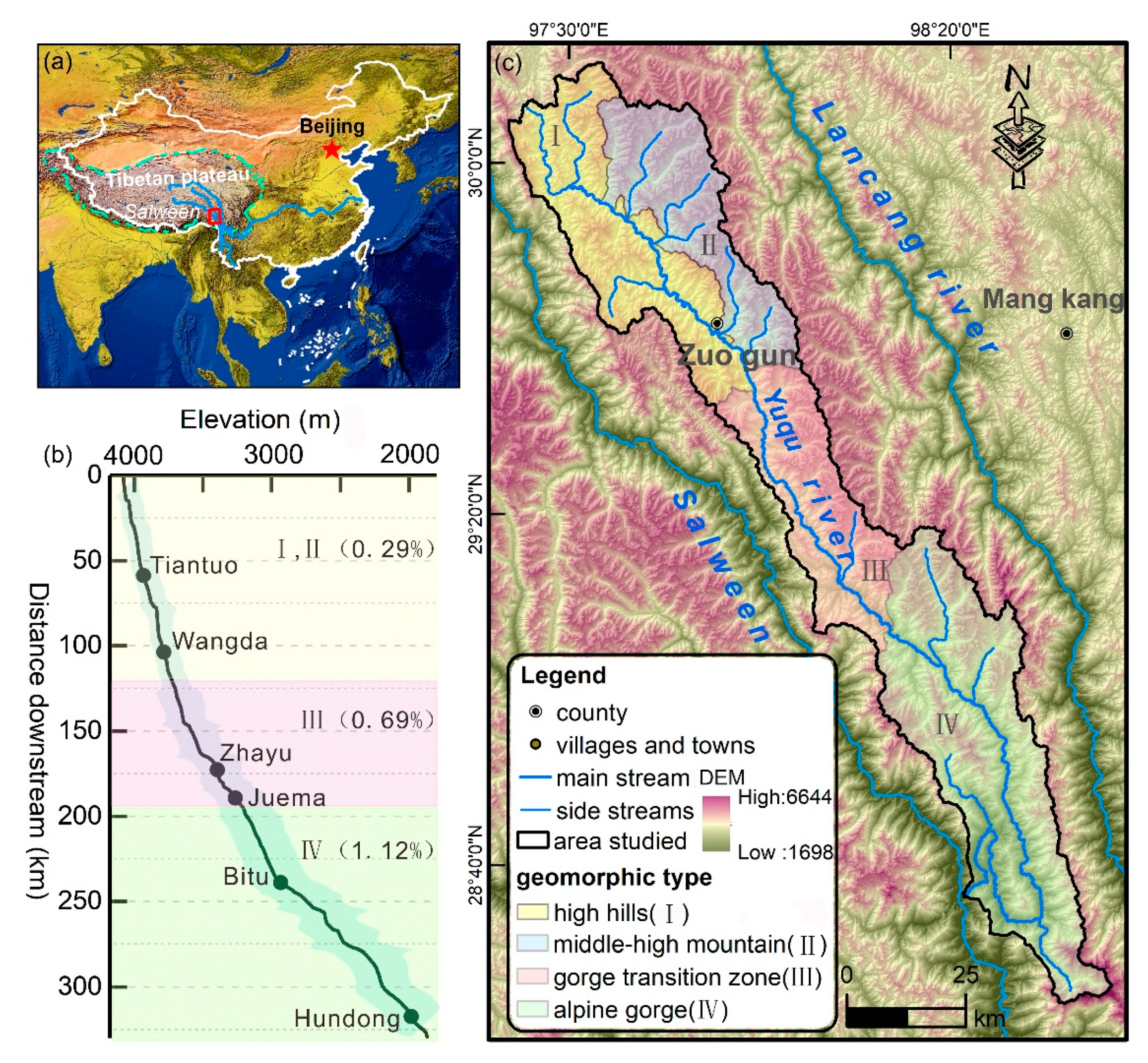
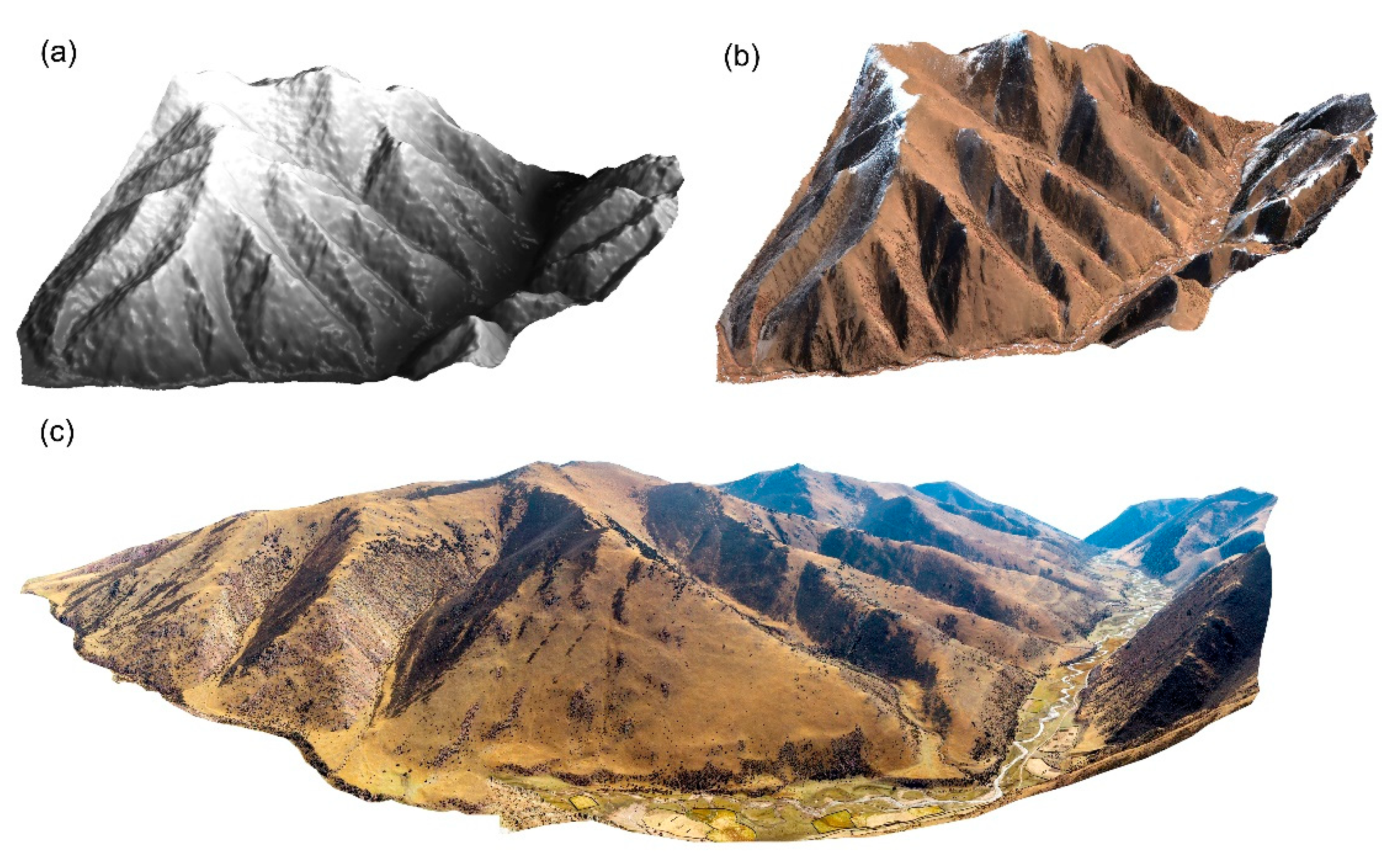
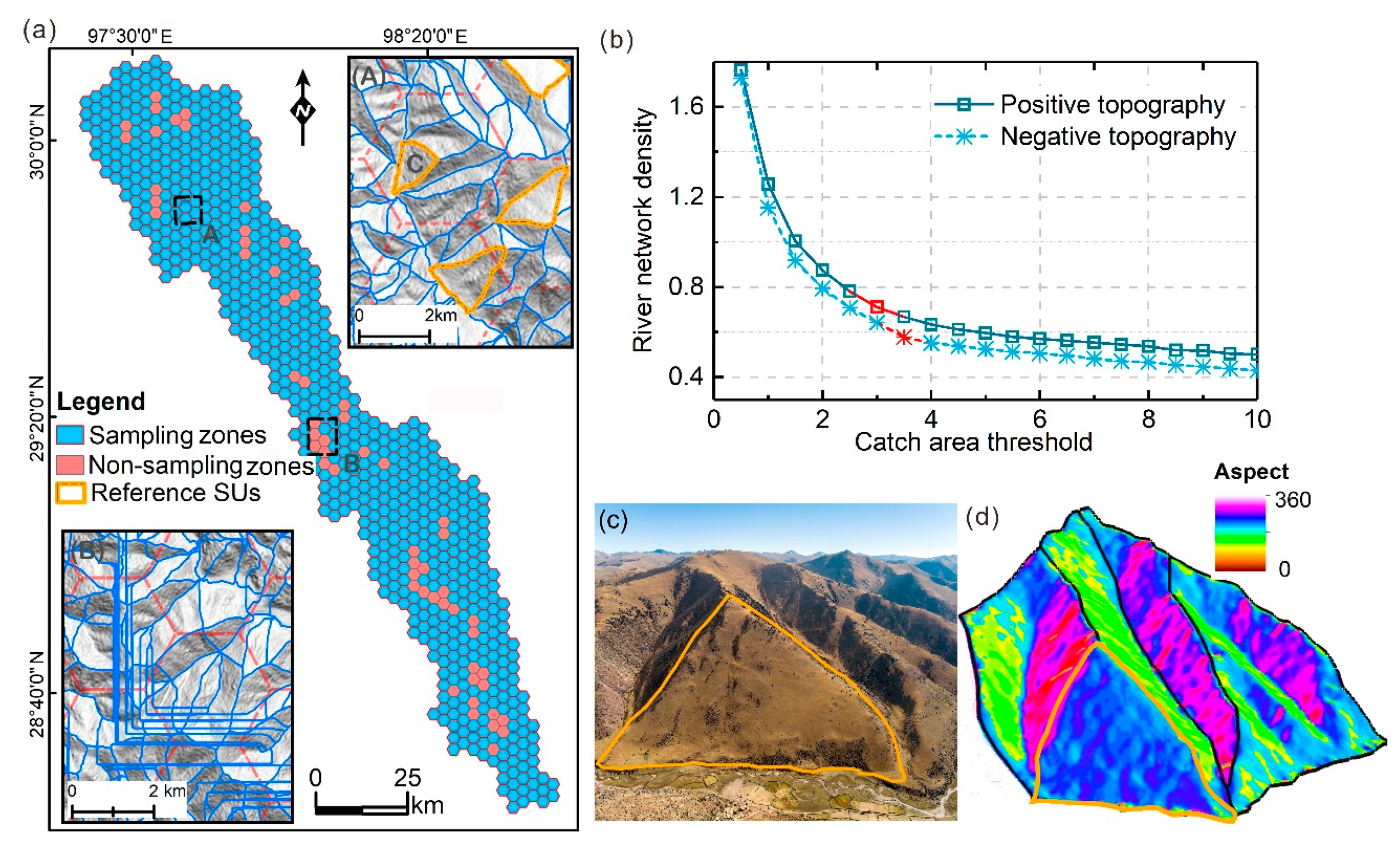
2.1. Study Area
2.2. Data Preparation
2.3. Reference SUs
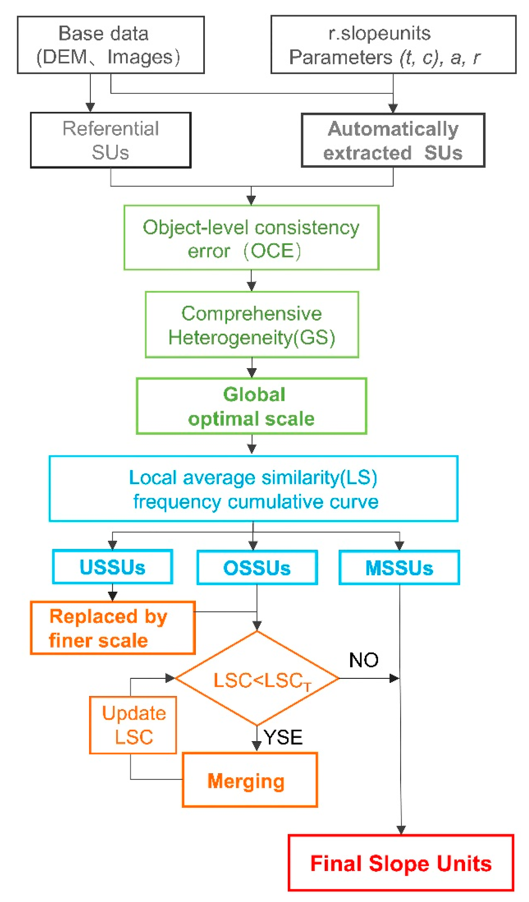
3. Methodology
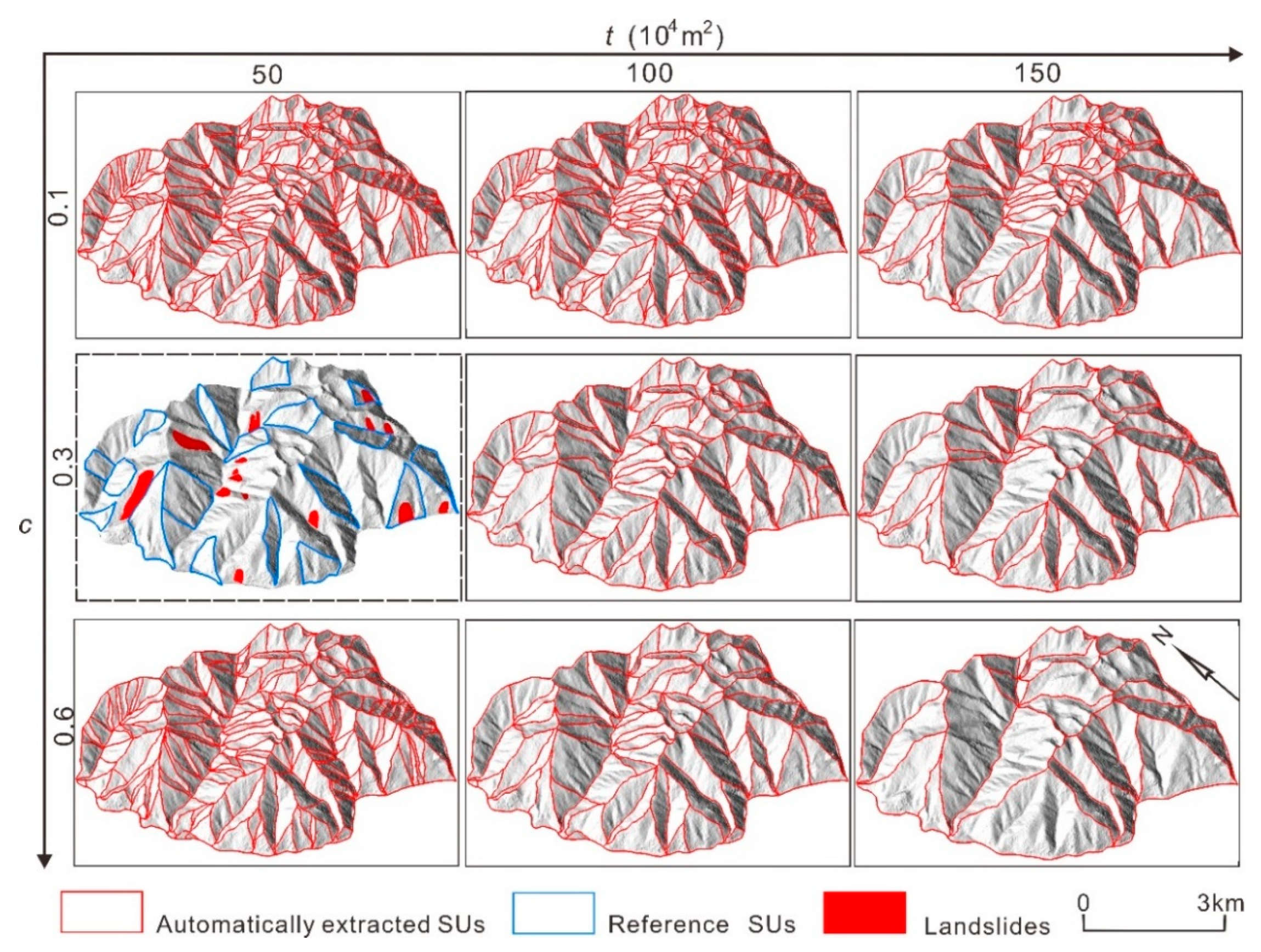
3.1. Initial Subdivision of SUs
3.2. Determination of the Optimal Subdivision Scale
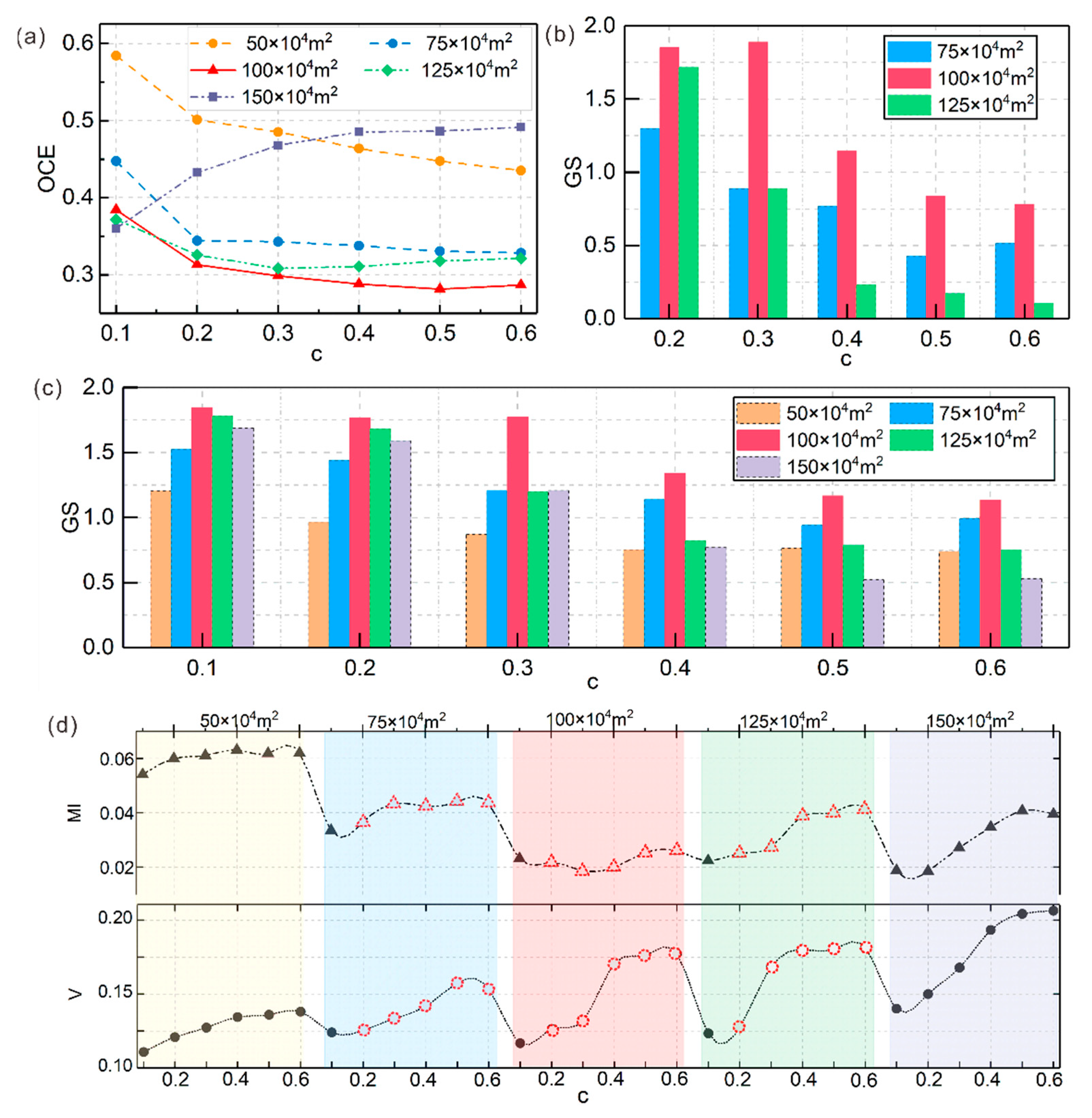
3.2.1. Object-Level Consistency Error ()
3.2.2. Global Optimal Heterogeneity
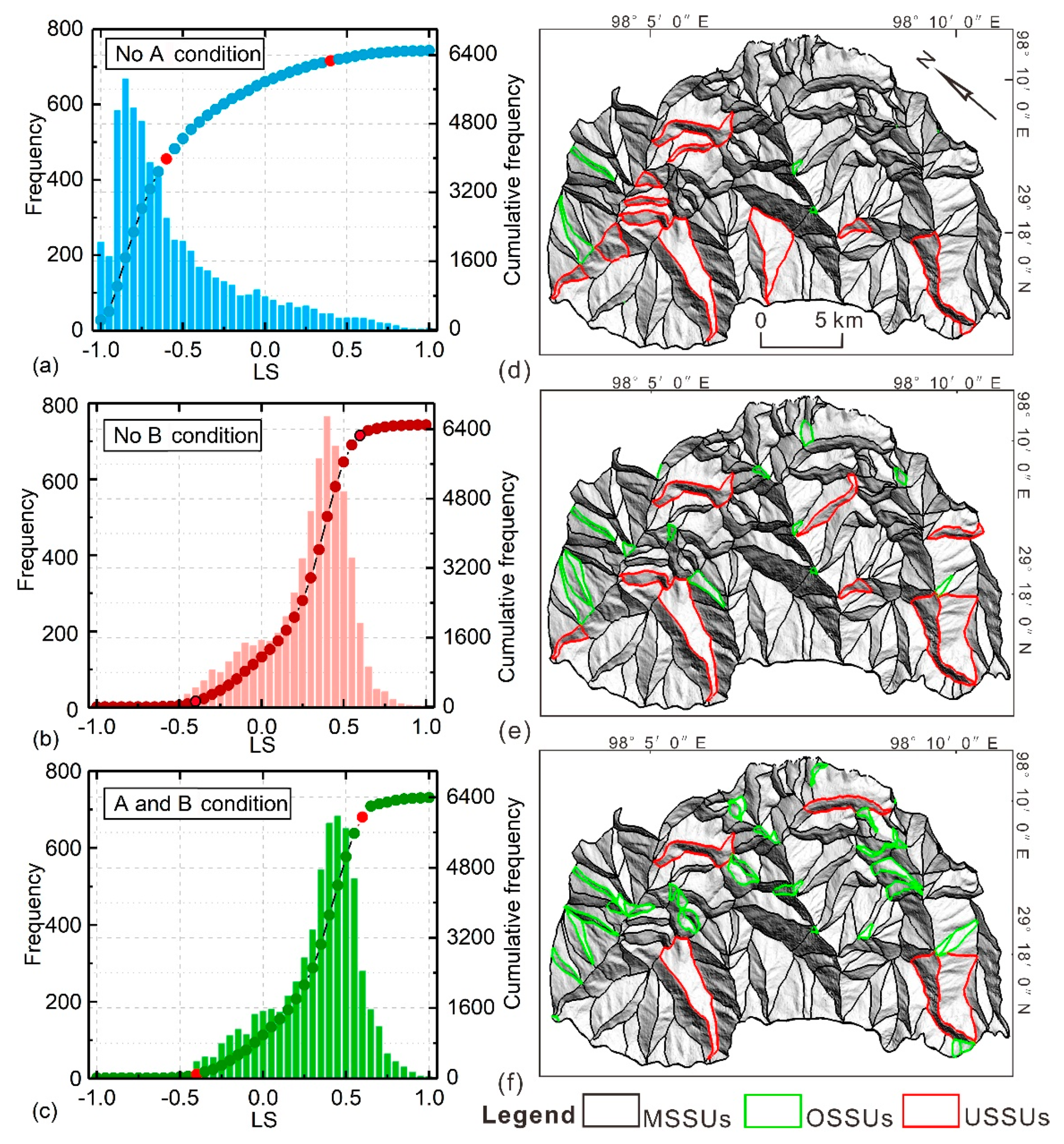
3.3. Identification of USSUs and OSSUs
3.4. The Optimization of USSUs and OSSUs
4. Results
4.1. Global Optimal Subdivision Scale
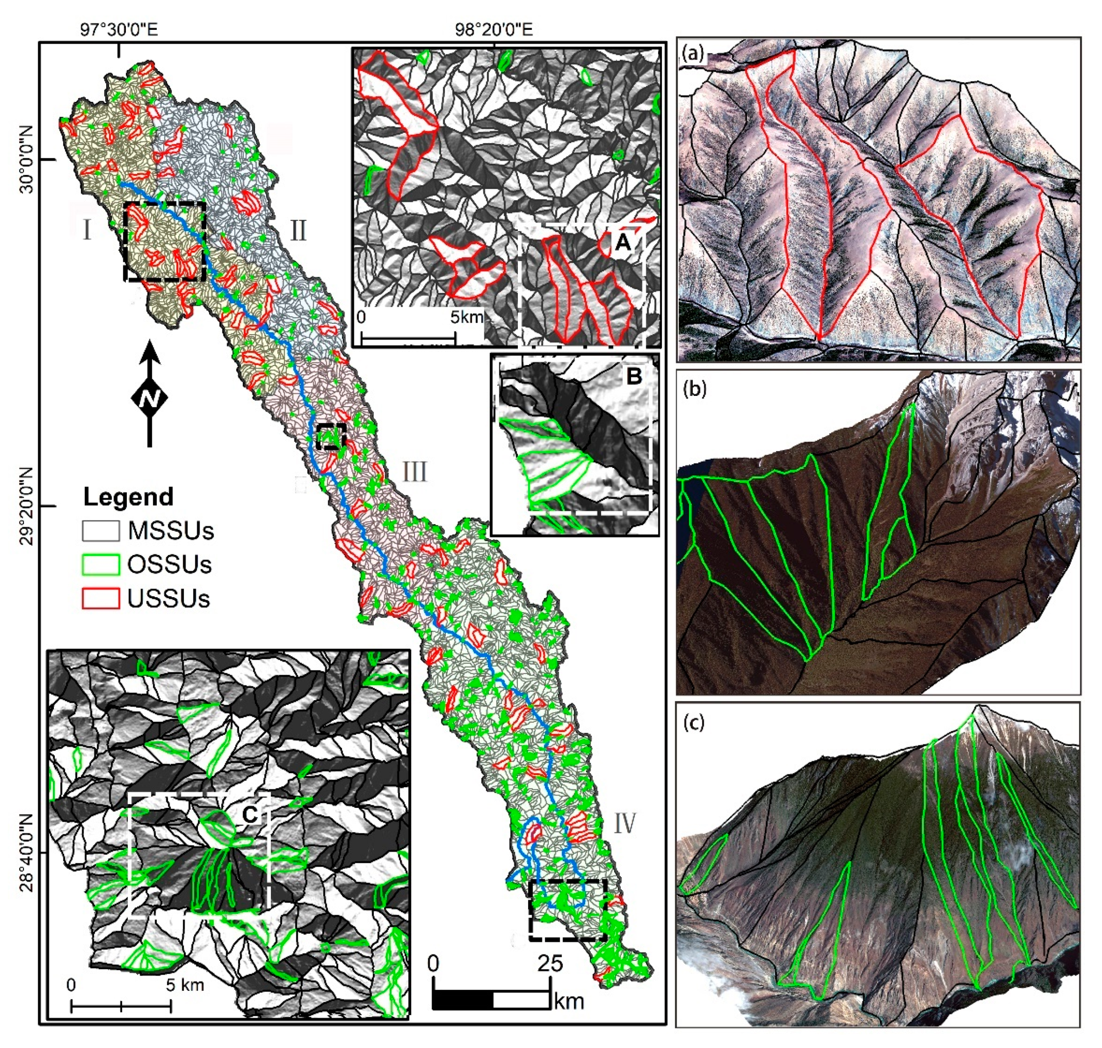
4.2. Identification Result of USSUs and OSSUs
4.3. Multi-Scale Optimization of Undesirable SUs
5. Discussion
5.1. Rationality of the Evaluation and Post-Processing for the Optimal Scale
5.2. Terrain-Adaptive Performance of the SUs Subdivision
6. Conclusions
Supplementary Materials
Author Contributions
Funding
Data Availability Statement
Conflicts of Interest
Abbreviations
| Variable | Description | First Introduced |
| a | Minimum surface area (m2) | r.slopeunits parameter |
| c | Minimum circular variance | r.slopeunits parameter |
| t | the initial flow accumulation area threshold (m2) | r.slopeunits parameter |
| r | Reduction factor | r.slopeunits parameter |
| the object-level consistency error | Equation (1) | |
| Moran’s I index | Equation (3) | |
| Variance index | Equation (4) | |
| the global heterogeneity score | Equation (5) | |
| the neighborhood variability of aspect difference | Equation (6) | |
| the neighborhood variability of the standard deviation | Equation (8) | |
| the area ratio of SU to its total area of adjacent units | Equation (9) | |
| the degree of coincidence of the common boundary | Equation (10) | |
| Local heterogeneity | Equation (11) | |
| Local homogeneity | Equation (12) | |
| the average local similarity | Equation (13) | |
| the average local similarity change | Equation (14) |
References
- Guzzetti, F.; Reichenbach, P.; Ardizzone, F.; Cardinali, M.; Galli, M. Estimating the quality of landslide susceptibility models. Geomorphology 2006, 81, 166–184. [Google Scholar] [CrossRef]
- Reichenbach, P.; Rossi, M.; Malamud, B.; Mihir, M.; Guzzetti, F. A review of statistically-based landslide susceptibility models. Earth-Sci. Rev. 2018, 180, 60–91. [Google Scholar] [CrossRef]
- Evans, I. Geomorphometry and landform mapping: What is a landform? Geomorphology 2012, 137, 94–106. [Google Scholar] [CrossRef]
- Xie, M.; Esaki, T.; Zhou, G. GIS-Based Probabilistic Mapping of Landslide Hazard Using a Three-Dimensional Deterministic Model. Nat. Hazards 2006, 33, 265–282. [Google Scholar] [CrossRef]
- Jacobs, L.; Kervyn, M.; Reichenbach, P.; Rossi, M.; Marchesini, I.; Alvioli, M.; Dewitte, O. Regional susceptibility assessments with heterogeneous landslide information: Slope unit- vs. pixel-based approach. Geomorphology 2020, 356, 107084. [Google Scholar] [CrossRef]
- Malamud, B.; Reichenbach, P.; Rossi, M.; Mihir, M. Report on Standards for Landslide Susceptibility Modelling and Terrain Zonations, LAMPRE FP7 Project Deliverables. 2014. Available online: http://www.lampre-project.eu (accessed on 3 November 2014).
- Minár, J.; Evans, I. Elementary forms for land surface segmentation: The theoretical basis of terrain analysis and geomorphological mapping. Geomorphology 2008, 95, 236–259. [Google Scholar] [CrossRef]
- Carrara, A.; Cardinali, M.; Detti, R.; Guzzetti, F.; Pasqui, V.; Reichenbach, P. GIS techniques and statistical models in evaluating landslide hazard. Earth Surf. Process. Landf. 1991, 16, 427–445. [Google Scholar] [CrossRef]
- Guzzetti, F.; Carrara, A.; Cardinali, M.; Reichenbach, P. Landslide hazard evaluation: A review of current techniques and their application in a multi-scale study, Central Italy. Geomorphology 1999, 31, 181–216. [Google Scholar] [CrossRef]
- Turel, M.; Frost, J. Delineation of Slope Profiles from Digital Elevation Models for Landslide Hazard Analysis. In Proceedings of the GeoRisk 2011: Geotechnical Risk Assessment and Management, Atlanta, GA, USA, 26–28 June 2011; American Society of Civil Engineers: Reston, WA, USA, 2011; pp. 829–836. [Google Scholar]
- Bornaetxea, T.; Rossi, M.; Marchesini, I.; Alvioli, M. Effective surveyed area and its role in statistical landslide susceptibility assessments. Nat. Hazards Earth Syst. Sci. 2018, 18, 2455–2469. [Google Scholar] [CrossRef] [Green Version]
- Xie, M.; Esaki, T.; Qiu, C.; Wang, C. Geographical information system-based computational implementation and application of spatial three-dimensional slope stability analysis. Comput. Geotech. 2006, 33, 260–274. [Google Scholar] [CrossRef]
- Romstad, B.; Etzelmuller, B. Mean-curvature watersheds: A simple method for segmentation of a digital elevation model into terrain units. Geomorphology 2012, 139, 293–302. [Google Scholar] [CrossRef] [Green Version]
- Alvioli, M.; Marchesini, I.; Reichenbach, P.; Rossi, M.; Ardizzone, F.; Fiorucci, F.; Guzzetti, F. Automatic delineation of geomorphological slope units with r.slopeunits v1.0 and their optimization for landslide susceptibility modeling. Geosci. Model Dev. 2016, 9, 3975–3991. [Google Scholar] [CrossRef] [Green Version]
- Alvioli, M.; Guzzetti, F.; Marchesini, I. Parameter-free delineation of slope units and terrain subdivision of Italy. Geomorphology 2020, 358, 107124. [Google Scholar] [CrossRef]
- Wang, K.; Zhang, S.; DelgadoTéllez, R.; Wei, F. A new slope unit extraction method for regional landslide analysis based on morphological image analysis. Bull. Eng. Geol. Environ. 2018, 78, 4139–4151. [Google Scholar] [CrossRef]
- Zhang, T.; Fu, Q.; Quevedo, R.; Chen, T.; Luo, D.; Liu, F.; Kong, H. Landslide Susceptibility Mapping Using Novel Hybrid Model Based on Different Mapping Units. KSCE J. Civ. Eng. 2022, 26, 2888–2900. [Google Scholar] [CrossRef]
- Huang, F.; Tao, S.; Chang, Z.; Huang, J.; Fan, X.; Jiang, S.; Li, W. Efficient and automatic extraction of slope units based on multi-scale segmentation method for landslide assessments. Landslides 2021, 18, 3715–3731. [Google Scholar] [CrossRef]
- Li, Y.; He, J.; Chen, F.; Han, Z.; Wang, W.; Chen, G.; Huang, J. Generation of Homogeneous Slope Units Using a Novel Object-Oriented Multi-Resolution Segmentation Method. Water 2021, 13, 3422. [Google Scholar] [CrossRef]
- Mergili, M.; Marchesini, I.; Alvioli, M.; Metz, M.; Schneider-Muntau, B.; Rossi, M.; Guzzetti, F. A strategy for GIS-based 3-D slope stability modelling over large areas. Geosci. Model Dev. 2014, 7, 2969–2982. [Google Scholar] [CrossRef] [Green Version]
- Dekavalla, M.; Argialas, D. Evaluation of a spatially adaptive approach for land surface classification from digital elevation models. Int. J. Geogr. Inf. Sci. 2017, 31, 1978–2000. [Google Scholar] [CrossRef]
- Zhao, M.; Li, F.; Tang, G. Optimal Scale Selection for DEM Based Slope Segmentation in the Loess Plateau. Int. J. Geosci. 2012, 3, 37–43. [Google Scholar] [CrossRef] [Green Version]
- Hu, Z.; Zhang, Q.; Zou, Q.; Li, Q.; Wu, G. Stepwise Evolution Analysis of the Region-Merging Segmentation for Scale Parameterization. IEEE J. Sel. Top. Appl. Earth Obs. Remote Sens. 2018, 11, 2461–2472. [Google Scholar] [CrossRef]
- Espindola, G.; Camara, G.; Reis, I.; Bins, L.; Monteiro, A. Parameter selection for region-growing image segmentation algorithms using spatial autocorrelation. Int. J. Remote Sens. 2006, 27, 3035–3040. [Google Scholar] [CrossRef]
- Polak, M.; Zhang, H.; Pi, M. An evaluation metric for image segmentation of multiple objects. Image Vis. Comput. 2009, 27, 1223–1227. [Google Scholar] [CrossRef]
- Hu, Z.; Li, Q.; Zhang, Q.; Zou, Q.; Wu, Z. Unsupervised Simplification of Image Hierarchies via Evolution Analysis in Scale-Sets Framework. IEEE Trans. Image Process. 2017, 26, 2394–2407. [Google Scholar] [CrossRef]
- Chen, J.; Deng, M.; Mei, X.; Chen, T.; Shao, Q.; Hong, L. Optimal segmentation of a high-resolution remote-sensing image guided by area and boundary. Int. J. Remote Sens. 2014, 35, 6914–6939. [Google Scholar] [CrossRef]
- Louw, G.; van Niekerk, A. Object-based land surface segmentation scale optimisation: An ill-structured problem. Geomorphology 2019, 327, 377–384. [Google Scholar] [CrossRef]
- Shi, X.; Li, Y.; Zhao, Q. Flexible Hierarchical Gaussian Mixture Model for High-Resolution Remote Sensing Image Segmentation. Remote Sens. 2020, 12, 1219. [Google Scholar] [CrossRef] [Green Version]
- Cheng, Y.; Mao, F. Selection of the Optimal Segmentation Scale in High-resolution Remote Sensing Image. DEStech Trans. Comput. Sci. Eng. 2018, 26, 1175–1184. [Google Scholar] [CrossRef] [Green Version]
- Dadgar, A.; Baleghi, Y.; Ezoji, M. Improved Object Matching in Multi-Objects Tracking Based on Zernike Moments and Combination of Multiple Similarity Metrics. Int. J. Eng. 2021, 34, 1445–1454. [Google Scholar] [CrossRef]
- Chen, F.; Liao, G. The Basic Geological Characteristics in Qamdo District. Contribution to the Geology of the Qinghai-Xizang (Tibet) Plateau, 1983; Geological Publishing House: Beijing, China, 1984; pp. 213–228. [Google Scholar]
- Zhang, W.; Tang, Q.; Liu, L.; Shen, J.; Li, Y.; Cheng, R. Geomorphologic analysis of Yuqu River Drainage basin in Tenasserim Chain Based on Hypsometric Integral Value. Sci. Geogr. Sin. 2020, 40, 1394–1402. [Google Scholar] [CrossRef]
- Zhao, Z.; Liu, Z.; Xu, C. Slope Unit-Based Landslide Susceptibility Mapping Using Certainty Factor, Support Vector Machine, Random Forest, CF-SVM and CF-RF Models. Front. Earth Sci. 2021, 9, 589630. [Google Scholar] [CrossRef]
- Wang, F.; Xu, P.; Wang, C.; Wang, N.; Jiang, N. Application of a GIS-Based Slope Unit Method for Landslide Susceptibility Mapping along the Longzi River, Southeastern Tibetan Plateau, China. ISPRS Int. J. Geo-Inf. 2017, 6, 172. [Google Scholar] [CrossRef] [Green Version]
- Sun, X.; Chen, J.; Han, X.; Bao, Y.; Zhu, X.; Peng, W. Landslide susceptibility mapping along the upper Jinsha River, south-western China: A comparison of hydrological and curvature watershed methods for slope unit classification. Bull. Eng. Geol. Environ. 2020, 79, 4657–4670. [Google Scholar] [CrossRef]
- Bellach, J.D.; Wayne, M. Biostatistics: A foundation for analysis in the health sciences, 4. ed. J. Wiley & Sons, New York–Chichester–Brisbane–Toronto–Singapore 1987, XIII, 734 S. S., $33.90. Biom. J. 2007, 30, 552. [Google Scholar] [CrossRef]
- Meng, T.; Xu, X.; Liu, H. Landslide risk assessment in high altitude areas based on slope unit optimization: Taking the Baige landslide in Jinsha River as an example. J. Henan Polytech. Univ. Nat. Sci. 2021, 40, 65–72. [Google Scholar] [CrossRef]
- Schlögel, R.; Marchesini, I.; Alvioli, M.; Reichenbach, P.; Rossi, M.; Malet, J. Optimizing landslide susceptibility zonation: Effects of DEM spatial resolution and slope unit delineation on logistic regression models. Geomorphology 2018, 301, 10–20. [Google Scholar] [CrossRef]
- Cai, Y.; Li, X.; Zhang, M.; Lin, H. Mapping wetland using the object-based stacked generalization method based on multi-temporal optical and SAR data. Int. J. Appl. Earth Obs. Geoinf. 2020, 92, 102164. [Google Scholar] [CrossRef]
- Yang, Z.; Wei, J.; Deng, J.; Gao, Y.; Zhao, S.; He, Z. Mapping Outburst Floods Using a Collaborative Learning Method Based on Temporally Dense Optical and SAR Data: A Case Study with the Baige Landslide Dam on the Jinsha River, Tibet. Remote Sens. 2021, 13, 2205. [Google Scholar] [CrossRef]
- Johnson, B.; Xie, Z. Unsupervised image segmentation evaluation and refinement using a multi-scale approach. ISPRS J. Photogramm. Remote Sens. 2011, 66, 473–483. [Google Scholar] [CrossRef]
- Otsu, N. A Threshold Selection Method from Gray-Level Histograms. IEEE Trans. Syst. Man Cybern. 1979, 9, 62–66. [Google Scholar] [CrossRef] [Green Version]
- Filali, I.; Allili, M.; Benblidia, N. Multi-scale salient object detection using graph ranking and global–local saliency refinement. Signal Processing Image Commun. 2016, 47, 380–401. [Google Scholar] [CrossRef]
- Zhao, S.; He, Z.; Deng, J.; Li, H.; Dai, F.; Gao, Y.; Chen, F. Giant river-blocking landslide dams with multiple failure sources in the Nu River and the impact on transient landscape evolution in southeastern Tibet. Geomorphology 2022, 413, 108357. [Google Scholar] [CrossRef]


| Parameters | Criterion | Reference |
|---|---|---|
| Filling threshold | (Positive topography) 40 m; (Negative topography) 60 m | [35,36,38] |
| Catchment area | (Positive topography) 3000 pixels; (Negative topography) 3500 pixels | [35,36,38] |
| Aspect circular variance | 0.20 ≤ ≤ 0.30 | [14,15,39] |
| Area | The maximum area of candidate reference SU in each sampling zone | [14] |
| Parameter | Value Setting |
|---|---|
| Initial flow accumulation threshold (t) | (50, 75, 100, 125, 150) × 104 m2 |
| Minimum circular variance (c) | (0.1, 0.2, 0.3, 0.4, 0.5, 0.6) |
| Minimum surface area (a) | 300,000 m2 |
| Reduction factor (r) | 11 |
| Cleaning size | 15,000 m2 |
| Feature Selection | USSUs Threshold | MSSUs Threshold | OSSUs Threshold | USSUs Percentage | OSSUs Percentage |
|---|---|---|---|---|---|
| No A | (−1.0~0.60) | (−0.60~0.90) | (0.90~1.0) | 61.14% | 4.28% |
| No B | (−1.0~0.35) | (−0.35~0.60) | (0.55~1.0) | 3.41% | 8.31% |
| A and B | (−1.0~0.40) | (−0.40~0.60) | (0.60~1.0) | 1.63% | 14.6% |
| Sequence | Total Number | New Completed | Not Done | Completed Proportion |
|---|---|---|---|---|
| Initial SUs | 0 | 1009 | 0% | |
| 1st merging | 1009 | 214 | 403 | 54.59% |
| 2rd merging | 617 | 138 | 179 | 89.79% |
| 3th merging | 531 | 27 | 40 | 96.68% |
| 4th merging | 419 | 9 | 6 | 98.97% |
| 5th merging | 398 | 4 | 0 | 100% |
| Total | 392 | 1637 |
| Classification | Initial State | Replacement | 1st Merging | 4th Merging | ||||
|---|---|---|---|---|---|---|---|---|
| Number | OCE | New SUs | Number | LSC < 0.5 | New SUs | LSC < 0.5 | OCE | |
| OSSUs | 952 | 0.30 | 0 | 1708 | 880 | 17 | 0 | 0.22 |
| USSUs | 106 | 756 | 415 | |||||
| MSSUs | 5456 | 0 | 5456 | 0 | 1100 | 0 | ||
| Total | 6514 | 756 | 7164 | 1295 | 1117 | 0 | ||
Publisher’s Note: MDPI stays neutral with regard to jurisdictional claims in published maps and institutional affiliations. |
© 2022 by the authors. Licensee MDPI, Basel, Switzerland. This article is an open access article distributed under the terms and conditions of the Creative Commons Attribution (CC BY) license (https://creativecommons.org/licenses/by/4.0/).
Share and Cite
Yang, Z.; Wei, J.; Deng, J.; Zhao, S. An Improved Method for the Evaluation and Local Multi-Scale Optimization of the Automatic Extraction of Slope Units in Complex Terrains. Remote Sens. 2022, 14, 3444. https://doi.org/10.3390/rs14143444
Yang Z, Wei J, Deng J, Zhao S. An Improved Method for the Evaluation and Local Multi-Scale Optimization of the Automatic Extraction of Slope Units in Complex Terrains. Remote Sensing. 2022; 14(14):3444. https://doi.org/10.3390/rs14143444
Chicago/Turabian StyleYang, Zhongkang, Jinbing Wei, Jianhui Deng, and Siyuan Zhao. 2022. "An Improved Method for the Evaluation and Local Multi-Scale Optimization of the Automatic Extraction of Slope Units in Complex Terrains" Remote Sensing 14, no. 14: 3444. https://doi.org/10.3390/rs14143444
APA StyleYang, Z., Wei, J., Deng, J., & Zhao, S. (2022). An Improved Method for the Evaluation and Local Multi-Scale Optimization of the Automatic Extraction of Slope Units in Complex Terrains. Remote Sensing, 14(14), 3444. https://doi.org/10.3390/rs14143444