Abstract
Geostatistical estimation methods rely on experimental variograms that are mostly erratic, leading to subjective model fitting and assuming normal distribution during conditional simulations. In contrast, Machine Learning Algorithms (MLA) are (1) free of such limitations, (2) can incorporate information from multiple sources and therefore emerge with increasing interest in real-time resource estimation and automation. However, MLAs need to be explored for robust learning of phenomena, better accuracy, and computational efficiency. This paper compares MLAs, i.e., Multiple Linear Regression (MLR) and Random Forest (RF), with Ordinary Kriging (OK). The techniques were applied to the publicly available Walkerlake dataset, while the exhaustive Walker Lake dataset was validated. The results of MLR were significant (p < 10 × 10−5), with correlation coefficients of 0.81 (R-square = 0.65) compared to 0.79 (R-square = 0.62) from the RF and OK methods. Additionally, MLR was automated (free from an intermediary step of variogram modelling as in OK), produced unbiased estimates, identified key samples representing different zones, and had higher computational efficiency.
1. Introduction
Estimation of attributes distributed in space is one of the most challenging problems in mining [1] (geochemical grades), petroleum [2] (porosity, permeability), environmental [3] (hazardous gases, substances), agricultural [4] (soil geochemistry, yield), geophysical [5] (resistivity signals), and other fields of Engineering [6,7]. Geostatistical techniques need to model spatial variability, i.e., subjective variogram model fitting to often erratic experimental variograms [8]. Geostatistical techniques assume stationarity assumptions and normalised data before conditional simulations [2,9,10,11]. Data for spatial estimation in the geoscience domain is obtained mostly through scarce and costly drilling methods [12,13,14,15]; therefore, robust MLAs must be explored. Real-time decision-making, particularly the demand for automation in various industries, requires efficient and less time-consuming spatial estimation models [16,17]. Unsupervised [8,18,19] and Supervised [8,20,21,22,23,24,25,26,27,28,29,30,31,32,33,34,35,36,37,38,39,40,41,42,43,44,45,46,47,48,49,50,51,52,53,54,55] Machine Learning Algorithms (MLAs) have been used as alternatives or as combination with geostatistical models, i.e., OK-Artificial Neural Network (ANN) [46]; Support Vector Machine (SVM) and Kriging [55]; ANN-Median Indicator Kriging (MIK) [56] for spatial interpolation in environmental sciences [44,57,58], weather forecasting [20,59,60], ecology [51,61,62], geography [28,32], landslides prediction [63,64,65], geochemical mapping [36,43,46,48], geophysical [66], mineral grade interpolation [8,21,45,47,55,67,68,69] etc. Neural network and their variants [29,34,53,54,70,71,72,73] have been widely used in numerous domains; they perform comparatively better but do not generalise well due to a shortage of training samples in spatial applications [74]. It is well established that neighbouring samples affect the interpolated grade at a given position/time; therefore, adding associated samples improves models’ performance [75,76]. Several RF-based spatial estimation algorithms have also been proposed in the literature [38,49,52,77]. This research explores MLAs that can incorporate all samples, capturing patterns globally at high computational efficiency. To further explore the MLAs, i.e., how and from which zones promising patterns are learnt, the SHapley Additive exPlanations (SHAP) algorithm [78,79] was used. In today’s era of automation and real-time optimisation/modelling [16,17], there is a need to explore novel Artificial Intelligence (AI) based spatial estimation techniques that can incorporate data from multiple sources with better accuracy, explainability, and computationally efficiency. The next section presents a literature review, a background of MLR, RF, and SHAP, followed by a case study, results, discussion, and conclusion.
2. Literature Review
Traditional spatial estimation techniques like polygonal, inverse distance, and power of inverse distance are geometrical methods replaced by probabilistic techniques like OK [80]. Most linear estimation techniques are a weighted linear combination of the surrounding sample values (e.g., % grade of metal in an ore deposit). Kriging is generally a particular case of the linear regression model [81]. The weights derived using the Kriging method rely on the variogram’s spatial structure, representing spatial autocorrelation of measured values from randomly distributed samples [11]. Simple Kriging (SK) assumes that the mean is known and constant; OK assumes that the mean is unknown and constant in the local neighbourhood; Universal Kriging (UK) assumes linear variation of mean in the spatial domain simultaneously while modelling spatial variability [11]. The UK may cause instability since the coordinates are considered simultaneously; therefore, researchers recommend modelling trend and residual components separately [31,82]. Kriging estimation also accounts for clustering in samples; and reports estimation variance, which is used for modelling uncertainty through conditional simulations in addition to short-scale variability [83].
MLR has been widely used for spatial estimation in different forms. For example, a MLR method estimated environmental variables at a coarser scale and then at a finer local scale [84]. Several other variants include clustering-based regression [85]; autoregression local linear regression of derivative of previously known values [86]; and nonlinear regression by spatial weight matrix [87]. A linear regression solution reducing the problem set by eigen analysis [88], and factor analysis [82] has also been reported. Various algorithms are compared as combinations represent the trend and residual models separately; the average grade from the best of these combinations is used to report the final estimates [31].
To avoid intermittent, manual, and subjective variogram modelling Neural Network-based hybrid fuzzy logic-genetic algorithm [89], genetic algorithm [34], and bee colony [70] based parameter optimisation has been used for spatial estimation. RF algorithm has been reported to perform better than the spatial linear regression model [38,81] even with very few samples, e.g., to predict copper mineralisation using 8 Geological features and two trace elements [35]. RF has proved as a flexible way of incorporating, combining, and extending variables of different types, leading to an informative mapping of prediction error [37]. More recently, RF spatial interpolation used observations at the nearest locations and their distances from the prediction location [36,77]. Directional neighbourhood distances, i.e., upslope and downslope from observation points, could be used; however, the computational intensity grows exponentially with the increase of variables [51]. Therefore, Principal Component Analysis (PCA) was applied to distance metric from sample coordinates to reduce spatial dimensions for getting an RF-PCA model showing higher prediction performances in validation compared to other methods [90].
More suitable Machine Learning (ML) based spatial estimation techniques need to be developed that are accurate and can incorporate multiple features; however, without computational complexity. Other combinations of the terms in an MLR model may be explored, representing interactions that describe the process under consideration. Depending on the domain, various features could be generated; for example, neighbouring samples’ distances and grades could be vital in the spatial domain.
3. Materials and Methods
3.1. Multiple Linear Regression (MLR)
MLR [47,91,92] is a well-known technique that estimates p + 1 parameters defining a linear relationship between input feature/s ( and output attribute for given n samples
The model is valid under assumptions that the input features are independent (not highly correlated), the error should be constant (homoscedastic), independent, and normally distributed. The term can be ignored as uncorrelated noise, while other parameters are determined as:
where X is the matrix with a column of unity and Y represents the output column vector with the intercept parameter at the end of the column. A higher number of features help learn nonlinear relationships and enables MLR to grasp complex problems with high variability [47,48,49]. A linear spatial autoregressive model in Equation (3) below contains four terms as spatial autoregressive models with a spatial autoregressive error term (SAR-SAR) [93]. The terms consist of (1) weighted dependent variables on an area with associated neighbouring values, followed by two regressor terms, i.e., (2) spatially lagged variable of the dependent variable, (3) spatially lagged variables of some or all the exogenous variables, and (4) last two terms representing the spatial model for the stochastic disturbances [93].
These dependencies resulted in estimating parameters by the Ordinary Least Square method (OLS) [93], expressing the interactions among dependent variables, independent covariates, and error terms [94].
3.2. Random Forest Algorithm
Random forest is an MLA developed by Breiman [95], consisting of a collection of decision trees where each decision tree represents the arrangement of variables learned from the dataset. It is applied to discover data patterns from various fields for solving regression problems [47,48,49]. In a decision tree, an upside-down tree is constructed in a hierarchy by selecting the best attributes from the subsets of the sample data set sequentially (see Figure 1). The random forest being ensemble method uses bagging to combine multiple decision trees by reducing the overfitting and improving the validation accuracy of the individual tree decision [95].
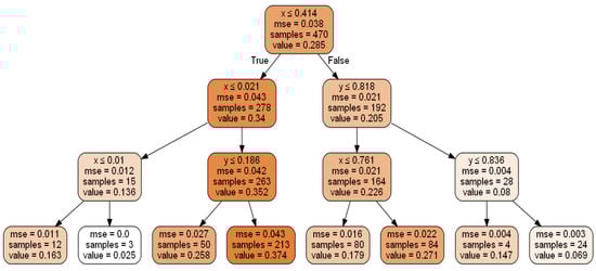
Figure 1.
Decision Tree having depth-4.
Figure 1 shows the decision tree for variable-V (e.g., output chemical concentration in ppm) prediction using sample data based on spatial positions (x and y). Some of the criteria used for stopping this process of tree construction are Max_depth (depth of the tree), Min_samples_leaf (minimum samples at leaf nodes), and threshold of a performance metric (Mean Absolute error (MAE)/Mean Squared Error (MSE)) [47,48,49]. The tree can be used to estimate values at an unknown point by asking questions on nodes; i.e., a query to the tree’s root node will lead through the intermediate nodes and finally to the leaf node, which represents the output, i.e., predicted value/class.
Each box in Figure 1 above represents a split of the sample data using:
- -row1: Best input attribute selected and its cutoff values in that subset
- -row2: Mean Squared Error for that subset
- -row3: Number of samples in that subset
- -row4: V (output e.g., chemical concentration) in that subset (the values are normalised between 0–1, which is not necessary for the decision tree).
The intensity of the colour shows the magnitude of the value of interest.
The best split (cut-off value) for the best input variable (spatial coordinate in the cartesian space) produces the most homogenous subgroups [96] in terms of the outputs (low, medium, or high-grade zones in this case). A suitable algorithm like Classification and Regression Tree (CART) would iteratively search for potential cut points, subdividing the data at each possible split for choosing the best split [97]. The decision tree depicted in Figure 1 has a depth of 4 levels. The root node is placed at level 1; levels 2 and 3 have the intermediate nodes, and leaf nodes with only output values are set at level 4. At level 1, the best attribute selected is x, and two subsets were created for level 2 based on the class values of x. At level 2, the best-chosen attributes for both subsets were x and y, respectively. Based on the importance of x and y in both subsets at level 2, further splitting was done into four subsets for level 3. At level 3, x was the best attribute for two subsets, whereas y was chosen as best for the other two subsets. Based on their respective subsets’ values, the dataset was further split into eight subsets for leaf nodes/level 4.
As seen in Figure 1, “x” and “y” are both critical spatial features for predicting output “V” by zoning the Walker Lake data in the cartesian space. This ability to find feature importance plays a crucial role when features increase significantly due to the availability of auxiliary information about the process. The decision tree identifies essential features and is intuitive since it explains the results in a set of if-then rules from top to bottom nodes; however, it suffers from lower validation accuracy and a higher chance of overfitting than other regression techniques [47,48,49].
A single tree would not produce a stable result for a new sample dataset; therefore, several trees are generated from a separate subset of random data drawn by replacement from a given dataset [47,48,49]. Random Forest overcomes the decision tree’s accuracy issue by fitting multiple trees through random resampling of the sample dataset with/without replacement. To produce generalised results, RF uses bagging for combining numerous trees, i.e., where the final predicted value is the average (in case of regression) or probability of occurrence (in case of classification) of the outputs from all trees [47,48,49]. A decision tree is also used as a base learner in ensemble methods such as Random Forest to improve hyperparameters and validation accuracy. Various decision tree hyperparameters such as Min_samples_leaf (minimum samples needed at a leaf node), Min_samples_split (minimum samples used for the splitting of the dataset), Max_features (maximum features allowed for the construction of tree), and Max_depth (maximum level of decision tree depth) are tuned to reduce overfitting.
3.3. Model Generalisation and Hyperparameter Tuning
Most MLA regression models suffer from “bias/under-fitting” or “variance/overfitting”; therefore, the main task is to find balance in-between by searching algorithm-specific hyperparameters. Hyperparameters are parameters associated with any regression model that cannot be learned from sample data and must be set before the fitting process [47,48,49]. Optimum hyperparameters are derived by providing a set of validation sample data that did not take part in training using the “cross-validation” or “hold-out” tuning [47,48,49,98]. After splitting the sample data, in case of hold-out or cross-validation, a hyperparameters search is usually done in a “grid” using a full factorial search.
A regression model is built for all combinations of hyperparameter ranges to find the best performing combination using a suitable validation strategy. The validation is a hold-out strategy when 20% of sample data for validation of the parameters, and a 10-fold validation, i.e., when ten subsets of data are used to verify the tuned parameters [47,48,49,98]. For example, in 10-fold cross-validation strategy, data is split into ten subsets while training on nine subsets and testing on the 10th subset; this process is repeated ten times, and each subset used for testing is different [47,48,49,98]. On the other hand, in the hold-out strategy, sample data is split randomly into two parts as 80:20, i.e., 80% of sample data is used for training and 20% for verification purposes during hyperparameters tuning. For both MLR and RF, the ten-fold cross-validation strategy was used to find the optimum regularisation values. Some authors have also used a combination of hold-out and cross-validation strategies [23,99,100,101,102,103]. However, the computational cost of grid search exponentially increases with the depth of hyperparameters search space, especially with a cross-validation strategy.
3.4. Performance Evaluation
All regression models express the inputs to output relationship by minimising an error metric (i.e., the dissimilarity between model output and the actual output) such as “Mean Squared Error (MSE)” or “Mean Absolute Error (MAE)” [47,48,49]. MSE and Root Mean Squared Error “RMSE” are differentiable, while MSE is more prone to outliers than RMSE and MAE [104]. The R-squared value is the complement of the ratio of the error variance = to the explained variance given as:
However, instead of using a single performance metric, such as correlation coefficient or R-squared value, researchers suggest using a “skill value” to combine the most critical performance metric as a summary statistic [24,25,105]. This term combines multiple important performance metrics such as “R_squared”, “Absolute Mean Error (AME)”, “Mean Absolute Error (MAE)”, and “Root Mean Square Error (RMSE)” [25]. The skill value can be presented as:
The best method is one with the lowest skill value.
3.5. Bayesian Optimisation Algorithm (BOA)
Regularisation is applied to find the best fit between low variance, i.e., underfitting, and high variance (i.e., overfitting). Best Hyperparameter values are searched using a Grid or Bayesian cross-validation strategy [47,48,49]. BOA [40,106,107,108] is an efficient method for finding hyperparameters using the Bayes theorem. According to the Bayes theorem, the conditional probability of an event is:
P(A|B) = P(B|A) ∗ P(A)/P(B)
The term P(B) is used for normalisation, which is not required in the case of optimisation. Hence, after dropping P(B), the posterior probability P(A|B) is a multiplication of likelihood P(B|A) and prior P(A). Possible hyperparameter samples (), and their evaluated cost from the objective function makes up data D and are used to calculate the prior. The likelihood function P(D|f) will change with more data collection, i.e., . The posterior probability, also called surrogate objective function P(f|D), represents the knowledge/approximation of the objective function, and will be used to evaluate the cost of various candidate samples using Equation (7) below.
P(f|D) = P(D|f) ∗ P(f)
The posterior probability is simply the product of likelihood and prior terms. The term ‘f’ represents the objective function to be maximised; D represents the data consisting of samples (different hyperparameter values (), evaluated/seen so far) and their associated costs . After fitting the function P(f|D) by a predictive modelling technique such as RF or gaussian process, the surrogate function, is used to test various candidate samples. A new set of hyperparameter values are sampled from the model using the Probability of Improvement (PI) given in Equation (8). If the PI is significant, the hyperparameters are used to determine their exact objective function value using 10-fold cross-validation, and the data is updated to remodel the function using Equation (7).
where cdf() = the normal cumulative distribution function, mu = the mean of surrogate function (P(f|D)) for a given sample x, stdev = the standard deviation of surrogate function for a given sample x, and best_mu = the mean of surrogate function for the best set of hyperparameters found so far.
PI = cdf((mu-best_mu)/stdev)
Stepwise detail of the BOA algorithm is described below: Initialisation: Generate data a set of hyperparameter values (), and associated objective function values , i.e., R-square values based on 10-fold cross validation from the RF/MLR algorithm).
For t = 1…N iterations
- 1.
- Model (P(f|Dt−1)) the objective function (R-square value) using Equation (7).
- 2.
- Find best_mu; i.e., the mean of the best values from the model (P(f|Dt−1))
- 3.
- Find a new set of best candidate/s (hyperparameter values) through PI
- 4.
- Compute the actual objective function/s by the RF/MLR algorithm, i.e., R-square value based on 10-fold cross-validation.
- 5.
- Update data as , i.e., and associated objective function values … and go to step 1
- 6.
- If PI is insignificant or N iterations are reached, stop and report the best parameters.
3.6. SHapley Additive ExPlanations (SHAP)
MLAs act as black-box models; therefore, interest is recently being developed among the artificial intelligence (AI) community to interpret the models using Explainable AI algorithms [78,80]. Such interpretations allow for a better understanding of inner mechanisms, resulting in more confidence in their application and usage [109]. SHAP algorithm [110] is widely used in various domains for interpreting MLAs [28,98] to determine the importance and effect of input features on output values.
The SHAP algorithm originated from cooperative game theory, where different players cooperate to increase the final payout. In the Machine Learning setting, the prediction task using a single dataset sample can be considered a game where various features (i.e., players) cooperate to play a game (i.e., predict output value). In the original form, the SHAP algorithm calculates the relative importance of different players by taking each player’s permutations in sequence and seeing the increment in payout each player makes. Similarly, each feature’s Shapley values can be calculated by taking all their permutations in series (for each sample) to quantify the difference in average prediction value and the prediction value for that specific sample. In other words, the Shapley value of each feature corresponds to the feature’s share of moving the sample prediction away from the average. Each feature’s global importance is reported by taking an average of the respective absolute Shapley values across the dataset. The greater the Shapley value, the greater the feature share, indicating that the feature is more critical for that single sample’s prediction task. The magnitude of feature importance Shapley values reports the importance, whereas the summary plot Shapley values indicate the effect on output. A positive value means a positive correlation between the feature value and the predicted attribute from average and vice versa.
3.7. The Walker Lake Dataset
This study uses the well-known Walker Lake dataset [11] from Nevada, western United States. Walker Lake dataset consists of two sets; Walker Lake survey data, having 470 samples, and exhaustively sampled data @ 1 × 1 m with 78,000 samples for the “V” variable, as shown in Figure 2 and Figure 3 (260 m × 300 m rectangular grid). Walker Lake survey and exhaustive data were used for training and validation purposes. Summary statistics for both survey and exhaustive data are shown in Table 1.
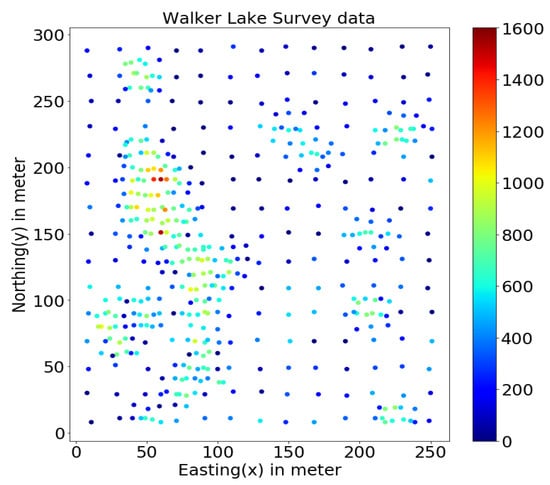
Figure 2.
Walker Lake survey data.
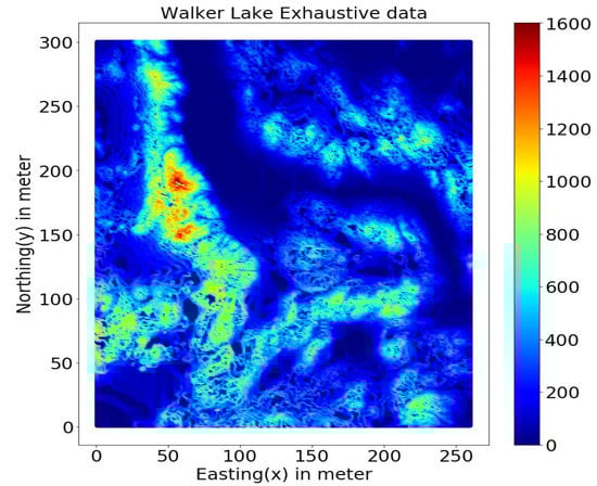
Figure 3.
Walker Lake exhaustive data.

Table 1.
Summary statistics Walker Lake data.
4. Application of MLR and RF for Spatial Estimation
After removing the trend, OK was applied to model the residual components to which the trend was added back for reporting the final OK estimates. The 470 samples were used to make omnidirectional and directional variograms of the residuals in 0, 45, 90, and 135 azimuths + tolerance of 22.5 degrees. OK estimates of the residuals were determined to estimate 78,000 points using the SGeMS software [11].
In the case of the MLA (MLR and RF models); the first step was to generate n + N input features for the estimation of each point from sample data, i.e., 472, for the given n = 2 (Easting and Northing coordinates) and N = 470 (distances of the 470 samples from this point). As a result, both MLR and RF (Figure 4) used n + N input features as N distances of all available samples from the point of estimation and n spatial coordinate dimensions of the point of estimation, as shown in Figure 5. All analyses, modelling, and visualisation tasks were done using numPy, pandas, scikit-learn, skopt, shap; and matplotlib libraries of Python [111]. Furthermore, BOA and the grid search made hyperparameter selection for MLR and RF was made using 10-fold cross-validation.
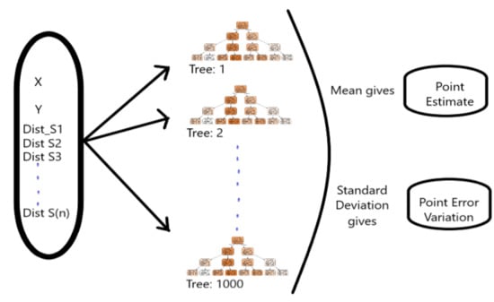
Figure 4.
Random Forest Model.
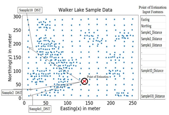
Figure 5.
Input Features for Point Estimation.
Optimum hyperparameters were searched using the Grid search and a BOA, i.e., an informed search method that optimises black-box functions in minimum time using information from previous iterations. Grid search was done as a full factorial search for comparison considering all combinations between the extreme values of various hyperparameters given in Table 2 and Table 3 for RF and MLR, respectively. The performance (R-square values) using ten-fold cross-validation were stored for each combination during the grid search. The “BayesSearchCV” class inside the “skopt” package of Python was also used to apply Bayesian optimisation of hyperparameters. Various hyperparameters of Random Forest, such as the minimum number of samples to be allowed at the leaf (Min_samples_leaf), maximum allowed depth of a tree (Max_depth), the maximum number of features to be used (Max_features), minimum number of samples to be used for splitting (Min_samples_split), and choice of a type of distance metric such as ‘Euclidean’, ’Squared Euclidean’, ’Minkowski’, ’Mahlanobis’, ’Cosine’, ‘Manhattan’, and ‘Chebyshev’ were tuned to obtain best results. Usually, the more than 128 trees do not improve performance significantly [112]; however, the number of trees parameter is also chosen as a hyperparameter. The Min_samples_leaf, Max_depth, Max_features and Min_samples_split were searched with an increment of 5%; while the Number of Trees was searched with an increment of 100 for ranges shown in Table 2.
Table 2.
The RF Hyper-Parameters ranges are used for searching the optimum values.
Table 3.
MLR HyperParameters range used for searching the optimum.
For MLR Regularisation parameter was searched from 0 to 1 with an increment of 0.05 along with various combinations of distances shown in Table 3.
The parameters reporting the best correlation coefficient value were chosen as optimum parameters used to train models (MLR and RF) utilising the entire 470 sample set. Lastly, the estimation methods had to be exact interpolators at known sample locations; therefore, the points precisely located on sample positions, i.e., 0 distances, were assigned the same grades to force exact interpolation.
5. Results
The trend component, as shown in Figure 6, was modelled by using the following linear regression Equation (9) using the cartesian coordinates Easting (X) and Northing (Y):
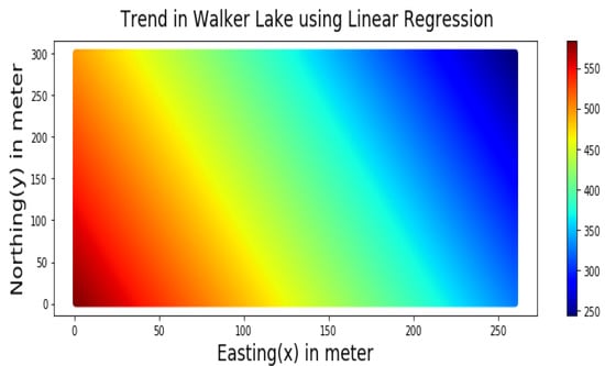
Figure 6.
Trend of the V variable of Walker Lake dataset represented by Equation (9).
After removing the trend, OK was used to model the residual components. The 470 samples were used to make omnidirectional and directional variograms with 0, 45, 90, and 135 azimuths + a tolerance of 22.5, as shown in Figure 7. OK weights were determined to estimate 78,000 points using the SGeMS software [11]. The directional variograms were modelled with the sill, nugget, and range values as 77,000, 20,000, and (min = 6, med = 28.8, max = 64.8), respectively, as shown in Figure 7.
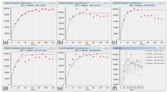
Figure 7.
Experimental and modeled variogram models for Walkerlake data; from top left to bottom right in (a) 0, (b) 45, (c) 90 and (d) 135 degrees Azimuth including (e) an omnidirectional and (f) variograms in all directions.
After finding the best regularisation parameter for the MLR using the Grid (taking two minutes) and BOA (within one minute), results were generated and compared with ground truth (exhaustive) data containing 78,000 samples. For the RF, finding optimum hyper-parameters using the Grid search took about 10 h on a core i-7 processor @ 2.8 GHz. While the Bayesian optimisation of RF hyperparameters took only 100 iterations to converge within 20 min, reporting the same optimum hyperparameters values as in the case of grid search. The RF and MLR models’ optimum parameters using the Bayesian and Grid search are reported in Table 4 and Table 5.
Table 4.
Optimum Hyper-Parameters RF.
Table 5.
Optimum Hyper-Parameters MLR.
As suggested by the literature, decreasing Min_samples_leaf, Min_samples_split, and increasing Max_features, Max_depth values increased RF variance, enabling us to explain complex relationships [47,48,49]. The optimum hyperparameter values found make intuitive sense, as the task of capturing spatial patterns, in this case, is complex [49]. MLR shows the same behaviour with a regularisation value of 0.
Summary statistics for MLR, RF, OK point estimates, and the exhaustive datasets are shown in Table 6 and the Taylor diagram in Figure 8. The results obtained from MLR, RF, and OK techniques were compared with the exhaustive data for validation, as shown in Table 7. These tables show that simple MLR performed better than RF and OK, in terms of RMSE, R-squared value, and respective skill values of 294.03, 319.39, and 328.64, respectively. The MLR, RF, and OK point estimates are shown in Figure 9, Figure 10 and Figure 11.
Table 6.
Various Model Results on Validation data (78,000 points).
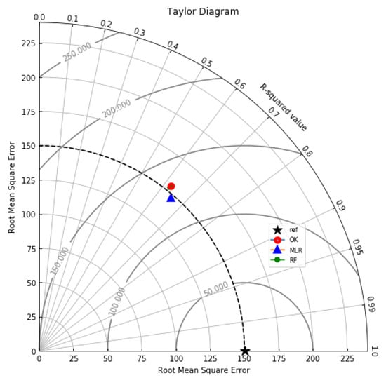
Figure 8.
Taylor diagram summarising the R-squared and RMSE of the OK, MLR and RF models.
Table 7.
Summary Statistics for Actual Exhaustive data vs. Models prediction.
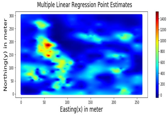
Figure 9.
Multiple Linear Regression Point Estimates for Walkerlake dataset.
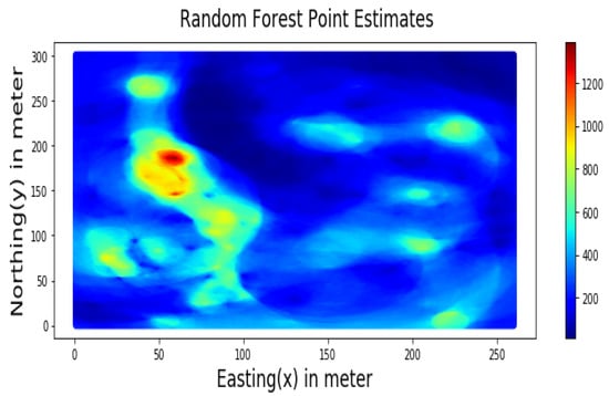
Figure 10.
RF-based Point Estimates for Walkerlake dataset.
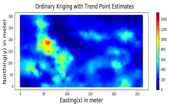
Figure 11.
Spatial Estimation of Walkerlake dataset by Ordinary Kriging.
Table 7 indicates that MLR point estimates distribution is closer to the actual (exhaustive) dataset than OK point estimates. MLR point estimates were unbiased, as evident from the mean values of MLR being closer to the exhaustive as given in Table 7. The “n” parameters associated with spatial coordinates model the linear trend simultaneously. In addition, the samples’ distances from the entire region are used as features by the “MLR”; in contrast, OK limits the use of neighbouring samples within the stationarity region, i.e., the variogram range. Therefore, the MLR allows itself to learn the nonlinear patterns from the closer and farther away samples.
Figure 12 shows the top 10 most important features (i.e., sample distances in this case) and their respective importance measures after applying the SHAP algorithm to the RF model. The distances reflect spatial locations of the top five features (i.e., the top five most influencing samples for each point to be estimated) shown in Figure 13, which are inside or at the boundaries of significant zones of interest (e.g., low, medium, high mineralisation zones). Therefore, identifying these zones of interest is paramount since this information plays a crucial role in spatial point estimations. Furthermore, it shows that distances of these samples from a given point of estimation in the entire domain are the most important during the estimation.
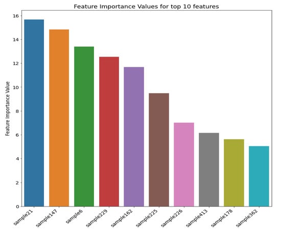
Figure 12.
Top 10 Features (samples) positively influencing the spatial estimation process in Walkerlake dataset.
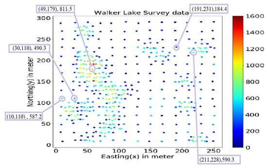
Figure 13.
Spatial location of top 5 Features positively influencing the estimation in Walkerlake dataset.
Similarly, samples inside major mineralisation zones have higher MLR coefficients, as shown in Figure 14. Therefore, for estimation problems involving a more significant number of samples, only cluster centres identified by the SHAP algorithm could be used as additional features instead of all sample distances.
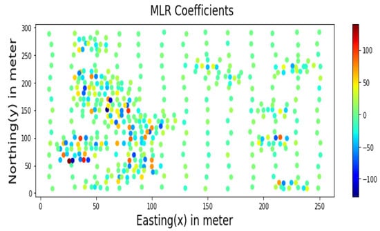
Figure 14.
MLR Coefficients for prediction using Walkerlake dataset.
It can be shown from the SHAP summary plot values (on the horizontal axis of Figure 15) of the twenty most influencing samples against the distance (red = greater and blue = smaller distance) each time taking part in estimating the 78,000 points. Suppose the higher grade/value sample lies closer (smaller distance indicated as blue) to a point being estimated; in that case, it has a positive SHAP value (likely to report higher estimates). Contrarily, if a higher grade/value sample is far (greater distance indicated as red) from the point being estimated, in that case, it is likely to report a negative SHAP value, i.e., lower estimates. The values for each sample distance were randomly increased and decreased to determine the effect on output point estimates. Intuitively, point estimates should reduce by increasing the distance from high-grade samples, indicating that increasing the distance from these samples results in lower estimation values, and closer distances from this point would report higher values. Conversely, negative SHAP values of high-grade samples at greater (red) distances, e.g., sample 6 and sample 21, indicate that lower grades will be reported at the estimation point at a greater distance from these high grades.
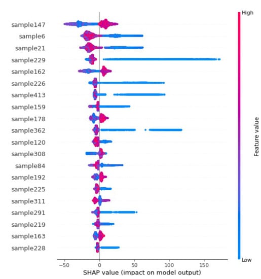
Figure 15.
Summary Plot of samples impact/influence on the estimation.
6. Discussion
Linear regression and RF algorithms have been applied using sample distances and spatial coordinates to estimate the value of interest in space. These estimates are an improvement over the previous linear estimation techniques since the samples’ distance features learn the variation of the correlations between the dependent, independent, and error terms. The algorithms reported greater computational efficiency than other techniques without loss of information through previously practiced feature reductions, e.g., PCA application to reduce features [90]. The MLR model was fast, unbiased, relatively accounted for short-scale variability, and can incorporate multiple data sources that can be used in real-time mining systems to perform resource estimation in an automated manner. Sample distances captured the spatial variability as additional features making even a simple linear regression model perform better than a complex nonlinear RF model. Out of the n + N parameters (n = sample coordinates and N = number of samples), the “n” parameters model the trend component and “N” parameters the variability across the domain. The results are aligned with those suggested by researchers [25,32,43,45,49], i.e., adding auxiliary information (regional anisotropies, mineralogy, and geophysical signals) improves the results. This research further performs estimation using maximum information with higher computational efficiency, particularly using MLR. The technique can be extended to other cases incorporating data from other sources to reinforce learned patterns. The algorithm shows the importance of using global information (i.e., all samples) to translate a highly nonlinear problem into a linear problem. These global indicators and thematic maps suggest that the MLR produced the most unbiased results and incorporated short-scale variability during estimation. Analysis of MLR coefficient values and sensitivity analysis of RF algorithm by SHAP algorithm reveals that key zones of interest (e.g., high, low medium mineralisation zones) were also identifiable during estimation. The coefficient values of MLR were derived by the gradient descent method, a default option in python libraries that were therefore not unstable. Hyperparameter tuning time was reduced significantly by the BOA compared to Grid search in the case of RF algorithm (20 min compared to 10 h) compared to MLR (one minute from two minutes). Therefore, MLR is a more significant improvement over both OK and RF algorithms producing better results (R-square of 0.652 compared to 0.62 for RF and OK) with significantly high computational efficiency.
Additionally, unlike previous estimations based on unsupervised methods [18,19] that identify different zones first to estimate grade values, the SHAP algorithm identified critical zones in the post-learning phase. This can be beneficial if the distances of most critical samples’ only could be used instead of all sample distances in exceptional circumstances involving huge samples to save computational cost. The technique could be explored further by applying a 3D case study, particularly for the mineral industry, to assess the estimates’ computational complexity, quality, and associated uncertainty. The variance of the estimates from MLR was higher than other methods, accounting for short-scale variability. However, reporting uncertainty of the estimates [36,113] is vital for sensitivity and risk analysis that can be explored in the next phase for comparing results with conditional simulations.
7. Conclusions
This paper compares Multiple Linear Regression (MLR), Random Forest (RF), and Ordinary Kriging (OK) using the sample and exhaustive Walkerlake dataset. Coordinates of the point of estimation and distances of the neighbouring samples were used as input features during the estimation. The global mean of the point estimates from the simple MLR method was unbiased, as evident from the corresponding Means of MLR, RF, OK, and Exhaustive datasets as 271.2, 288.2, 295.42, and 277.98. Apart from the relatively higher accuracy, the reported variance of 47,276.1 from MLR point estimates was closer to the variance of 62,423.2 from exhaustive data than that of 38,476.42 from OK, which indicates that MLR accounts for short-scale variability. Furthermore, estimates from simple MLR honoured global parameters of the exhaustive data, which may be due to the entire sample set being used as input, during point estimation, while kriging limits neighbouring information to the stationarity region, i.e., the variogram range. The proposed technique is computationally efficient, solving the prediction model within a second for estimating 78,000 points and automated, i.e., without manual interaction. MLR and RF algorithms revealed that the proposed method could be used as fast means of estimation since (1) these algorithms make use of the key zones of importance during point estimation; (2) In cases with a large number of sample points, only the most critical samples distances could be used as features instead of all sample distances.
Author Contributions
Conceptualization, Waqas Ahmed and Khan Muhammad; Formal analysis, Waqas Ahmed, Khan Muhammad, Hylke Jan Glass, Snehamoy Chatterjee and Asif Khan; Funding acquisition, Khan Muhammad and Asif Khan; Investigation, Waqas Ahmed, Khan Muhammad, Hylke Jan Glass and Snehamoy Chatterjee; Methodology, Waqas Ahmed and Khan Muhammad; Project administration, Khan Muhammad and Asif Khan; Resources, Khan Muhammad; Software, Waqas Ahmed, Abid Hussain and Khan Muhammad; Supervision, Khan Muhammad and Asif Khan; Validation, Waqas Ahmed and Khan Muhammad; Visualization, Waqas Ahmed; Writing—original draft, Waqas Ahmed, Khan Muhammad and Abid Hussain; Writing—review & editing, Khan Muhammad, Hylke Jan Glass and Snehamoy Chatterjee. All authors have read and agreed to the published version of the manuscript.
Funding
This research was funded by Higher Education Commission Pakistan through grant number ‘National Centre of Artificial Intelligence’ and the APC was funded by the authors.
Institutional Review Board Statement
Not applicable.
Informed Consent Statement
Not applicable.
Conflicts of Interest
The authors declare no conflict of interest.
References
- Rossi, M.E.; Deutsch, C.V. Mineral Resource Estimation; Springer: Dordrecht, The Netherlands, 2014; ISBN 9781402057175. [Google Scholar]
- Pyrcz, M.J.; Deutsch, C. Geostatistical Reservoir Modeling, 2nd ed.; Oxford University Press: New York, NY, USA, 2002; ISBN 0-19-513806-6. [Google Scholar]
- Monestiez, P.; Allard, D.; Froidevaux, R. geoENV III—Geostatistics for Environmental Applications. Proceedings of the Third European Conference on Geostatistics for Environmental Applications Held in Avignon, France, November 22–24; Springer: Dordrecht, The Netherlands, 2000; ISBN 978-0-7923-7107-6. [Google Scholar]
- Oliver, M.A. Geostatistical Applications for Precision Agriculture; Springer: New York, NY, USA, 2010; ISBN 978-90-481-9132-1. [Google Scholar]
- Azevedo, L.; Soares, A. Geostatistical Methods for Reservoir Geophysics; Springer: Cham, Switzerland, 2017; ISBN 978-3-319-53200-4. [Google Scholar]
- Leuangthong, O.; Khan, K.D.; Deutsch, C.V. Solved Problems in Geostatistics; Wiley: Hoboken, NJ, USA, 2008; ISBN 978-0-470-17792-1. [Google Scholar]
- Sarma, D. Geostatistics with Applications in Earth Sciences; Springer: Dordrecht, The Netherlands, 2006; ISBN 978-1-4020-9379-1. [Google Scholar]
- Pham, T.D. Grade estimation using fuzzy-set algorithms. Math. Geol. 1997, 29, 291–305. [Google Scholar] [CrossRef]
- Matheron, G. Principals of Geostatistics. Econ. Geol. 1962, 58, 1246–1266. [Google Scholar] [CrossRef]
- Kwon, H.; Yi, S.; Choi, S. Numerical investigation for erratic behavior of Kriging surrogate model. J. Mech. Sci. Technol. 2014, 28, 3697–3707. [Google Scholar] [CrossRef]
- Isaaks, E.H.; Srivastava, R.M. Applied Geostatistics, 1st ed.; Oxford University Press: New York, NY, USA, 1989; ISBN 978-0- 19-605013-4. [Google Scholar]
- Abedi, M.; Ali Torabi, S.; Norouzi, G.H.; Hamzeh, M.; Elyasi, G.R. PROMETHEE II: A knowledge-driven method for copper exploration. Comput. Geosci. 2012, 46, 255–263. [Google Scholar] [CrossRef]
- Dutaut, R.; Marcotte, D. A New Semi-greedy Approach to Enhance Drillhole Planning. Nat. Resour. Res. 2020, 29, 3599–3612. [Google Scholar] [CrossRef]
- Fatehi, M.; Asadi, H.H.; Hossein Morshedy, A. 3D Design of Optimum Complementary Boreholes by Integrated Analysis of Various Exploratory Data Using a Sequential-MADM Approach. Nat. Resour. Res. 2020, 29, 1041–1061. [Google Scholar] [CrossRef]
- Kumral, M.; Ozer, U. Computers & Geosciences Planning additional drilling campaign using two-space genetic algorithm: A game theoretical approach. Comput. Geosci. 2013, 52, 117–125. [Google Scholar] [CrossRef]
- Benndorf, J. Moving towards Real-Time Management of Mineral Reserves—A Geostatistical and Mine Optimization Closed-Loop Framework. In Mine Planning and Equipment Selection.; Drebenstedt, C., Singhal, R., Eds.; Springer International Publishing: Cham, Switzerland, 2014; pp. 989–999. ISBN 978-3-319-02678-7. [Google Scholar]
- Buxton, M.; Benndorf, J. The use of sensor derived data in optimisation along the Mine-Value-Chain. In Proceedings of the 15th International ISM Congress, Aachen, Germany, 16–20 September 2013; pp. 324–336. [Google Scholar]
- Muhammad, K.; Glass, H.J. Modelling Short-Scale Variability and Uncertainty During Mineral Resource Estimation Using a Novel Fuzzy Estimation Technique. Geostand. Geoanalytical Res. 2011, 35, 369–385. [Google Scholar] [CrossRef]
- Tutmez, B.; Tercan, A.E.; Kaymak, U.; Appelhans, T.; Mwangomo, E.; Hardy, D.R.; Hemp, A.; Nauss, T.; Tutmez, B.; Tercan, A.E.; et al. Fuzzy Modeling for Reserve Estimation Based on Spatial Variability. Math. Geol. 2007, 39, 87–111. [Google Scholar] [CrossRef]
- Appelhans, T.; Mwangomo, E.; Hardy, D.R.; Hemp, A.; Nauss, T. Evaluating machine learning approaches for the interpolation of monthly air temperature at Mt. Kilimanjaro, Tanzania. Spat. Stat. 2015, 14, 91–113. [Google Scholar] [CrossRef]
- Kapageridis, I.K.; Denby, B. Neural Network Modelling of Ore Grade Spatial Variability. In Perspectives in Neural Computing, Proceedings of the ICANN, Skovde, Sweden, 2–4 September 1998; Niklasson, L., Bodén, M., Ziemke, T., Eds.; Springer: London, UK, 1998; pp. 209–214. [Google Scholar]
- Dean, S. Journal of Natural Gas Science and Engineering Reservoir simulation and modeling based on artificial intelligence and data. J. Nat. Gas Sci. Eng. 2011, 3, 697–705. [Google Scholar] [CrossRef]
- Dou, J.; Yunus, A.P.; Tien Bui, D.; Merghadi, A.; Sahana, M.; Zhu, Z.; Chen, C.W.; Khosravi, K.; Yang, Y.; Pham, B.T. Assessment of advanced random forest and decision tree algorithms for modeling rainfall-induced landslide susceptibility in the Izu-Oshima Volcanic Island, Japan. Sci. Total Environ. 2019, 662, 332–346. [Google Scholar] [CrossRef]
- Dutta, S. Predictive Performance of Machine Learning Algorithms for Ore Reserve Estimation in Sparse and Imprecise Data. Ph.D. Thesis, University of Alaska Fairbanks, Fairbanks, AK, USA, 2006. [Google Scholar]
- Dutta, S.; Bandopadhyay, S.; Ganguli, R.; Misra, D. Machine Learning Algorithms and Their Application to Ore Reserve Estimation of Sparse and Imprecise Data. J. Intell. Learn. Syst. Appl. 2010, 2, 86–96. [Google Scholar] [CrossRef]
- Gilardi, N.; Bengio, S. Comparison of four machine learning algorithms for spatial data analysis. In Mapping radioactivity in the environment—Spatial Interpolation Comparison 1997; Dubois, G., Malczewski, J., DeCort, M., Eds.; Office for Official Publications of the European Communities: Luxembourg, 2003; pp. 222–237. [Google Scholar]
- Gonçalves, Í.G.; Kumaira, S.; Guadagnin, F. Computers & Geosciences A machine learning approach to the potential- fi eld method for implicit modeling of geological structures. Comput. Geosci. 2017, 103, 173–182. [Google Scholar] [CrossRef]
- Gumus, K.; Sen, A. Comparison of spatial interpolation methods and multi-layer neural networks for different point distributions on a digital elevation model. Geod. Vestn. 2013, 57, 523–543. [Google Scholar] [CrossRef]
- Koike, K.; Matsuda, S.; Suzuki, T.; Ohmi, M. Neural Network-Based Estimation of Principal Metal Contents in the Hokuroku District, Northern Japan, for Exploring Kuroko-Type Deposits. Nat. Resour. Res. 2002, 11, 135–156. [Google Scholar] [CrossRef]
- Leone, S.; Rutile, S.; Limited, C.; Leone, S. Integrating artificial neural networks and geostatistics for optimum 3D geological block modelling in mineral reserve estimation—A case study. Int. J. Min. Sci. Technol. 2015, 26, 581–585. [Google Scholar]
- Li, J.; Heap, A.D.; Potter, A.; Daniell, J.J. Application of machine learning methods to spatial interpolation of environmental variables. Environ. Model. Softw. 2011, 26, 1647–1659. [Google Scholar] [CrossRef]
- Merwin, D.A.; Cromley, R.G.; Civco, D.L. Artificial neural networks as a method of spatial interpolation for digital elevation models. Cartogr. Geogr. Inf. Sci. 2002, 29, 99–110. [Google Scholar] [CrossRef]
- Rigol, J.P.; Jarvis, C.H.; Stuart, N. Artificial neural networks as a tool for spatial interpolation. Int. J. Geogr. Inf. Sci. 2001, 15, 323–343. [Google Scholar] [CrossRef]
- Yadav, A.; Satyannarayana, P. Multi-objective genetic algorithm optimisation of artificial neural network for estimating suspended sediment yield in Mahanadi River basin, India. Int. J. River Basin Manag. 2020, 18, 207–215. [Google Scholar] [CrossRef]
- Carranza, E.J.M.; Laborte, A.G. Random Forest Predictive Modeling of Mineral Prospectivity with Missing Values in Abra (Philippines). Comput. Geosci. 2015, 74, 60–70. [Google Scholar] [CrossRef]
- Veronesi, F.; Schillaci, C. Comparison between geostatistical and machine learning models as predictors of topsoil organic carbon with a focus on local uncertainty estimation. Ecol. Indic. 2019, 101, 1032–1044. [Google Scholar] [CrossRef]
- Hengl, T.; Nussbaum, M.; Wright, M.N.; Heuvelink, G.B.M.; Gräler, B. Random forest as a generic framework for predictive modeling of spatial and spatio-temporal variables. PeerJ 2018, 2018, e5518. [Google Scholar] [CrossRef]
- Baez-Villanueva, O.M.; Zambrano-Bigiarini, M.; Beck, H.E.; McNamara, I.; Ribbe, L.; Nauditt, A.; Birkel, C.; Verbist, K.; Giraldo-Osorio, J.D.; Xuan Thinh, N. RF-MEP: A novel Random Forest method for merging gridded precipitation products and ground-based measurements. Remote Sens. Environ. 2020, 239, 111606. [Google Scholar] [CrossRef]
- Fiorentini, N.; Maboudi, M.; Losa, M.; Gerke, M. Assessing resilience of infrastructures towards exogenous events by using ps-insar-based surface motion estimates and machine learning regression techniques. ISPRS Ann. Photogramm. Remote Sens. Spat. Inf. Sci. 2020, 5, 19–26. [Google Scholar] [CrossRef]
- Fiorentini, N.; Maboudi, M.; Leandri, P.; Losa, M.; Gerke, M. Surface motion prediction and mapping for road infrastructures management by PS-InSAR measurements and machine learning algorithms. Remote Sens. 2020, 12, 3976. [Google Scholar] [CrossRef]
- Xie, Z.; Chen, G.; Meng, X.; Zhang, Y.; Qiao, L.; Tan, L. A comparative study of landslide susceptibility mapping using weight of evidence, logistic regression and support vector machine and evaluated by SBAS-InSAR monitoring: Zhouqu to Wudu segment in Bailong River Basin, China. Environ. Earth Sci. 2017, 76, 313. [Google Scholar] [CrossRef]
- Lesniak, A.; Porzycka, S. Geostatistical computing in psinsar data analysis. In Computational Science—ICCS 2009; Allen, G., Nabrzyski, J., Seidel, E., van Albada, G.D., Dongarra, J., Sloot, P.M.A., Eds.; Lecture Notes in Computer Science; Springer: Berlin/Heidelberg, Germany, 2009; Volume 5544. [Google Scholar] [CrossRef]
- Liu, W.; Du, P.; Wang, D. Ensemble learning for spatial interpolation of soil potassium content based on environmental information. PLoS ONE 2015, 10, e0124383. [Google Scholar] [CrossRef]
- Liu, S.; Zhang, Y.; Ma, P.; Lu, B.; Su, H. A Novel Spatial Interpolation Method Based on the Integrated RBF Neural Network. Procedia Environ. Sci. 2011, 10, 568–575. [Google Scholar] [CrossRef]
- Kirkwood, C.; Cave, M.; Beamish, D.; Grebby, S.; Ferreira, A. A machine learning approach to geochemical mapping. J. Geochem. Explor. 2016, 167, 49–61. [Google Scholar] [CrossRef]
- Dai, F.; Zhou, Q.; Lv, Z.; Wang, X.; Liu, G. Spatial prediction of soil organic matter content integrating artificial neural network and ordinary kriging in Tibetan Plateau. Ecol. Indic. 2014, 45, 184–194. [Google Scholar] [CrossRef]
- Hastie, T.; Tibshirani, R.; Friedman, J. The Elements of Statistical Learning Data Mining, Inference, and Prediction, 2nd ed.; Series in Statistics; Springer: New York, NY, USA, 2009; ISBN 978-0-387-84857-0. [Google Scholar]
- Bishop, C.M. Pattern Recognition and Machine Learning; Springer: New York, NY, USA, 2006; Volume 2, ISBN 9780387310732. [Google Scholar]
- Russell, S.J.; Norvig, P. Artificial Intelligence A Modern Approach 4th Edition, 3rd ed.; Prentice Hall: Hoboken, NJ, USA, 2003; ISBN 9780136042594. [Google Scholar]
- Anees, M.T.; Abdullah, K.; Nawawi, M.N.M.; Ab Rahman, N.N.N.; Piah, A.R., Mt.; Syakir, M.I.; Ali Khan, M.M.; Abdul, A.K. Spatial estimation of average daily precipitation using multiple linear regression by using topographic and wind speed variables in tropical climate. J. Environ. Eng. Landsc. Manag. 2018, 26, 299–316. [Google Scholar] [CrossRef]
- Baltensperger, A.P.; Mullet, T.C.; Schmid, M.S.; Humphries, G.R.W.; Kövér, L.; Huettmann, F. Seasonal observations and machine-learning-based spatial model predictions for the common raven (Corvus corax) in the urban, sub-arctic environment of Fairbanks, Alaska. Polar Biol. 2013, 36, 1587–1599. [Google Scholar] [CrossRef]
- Bel, L.; Allard, D.; Laurent, J.M.; Cheddadi, R.; Bar-Hen, A. CART algorithm for spatial data: Application to environmental and ecological data. Comput. Stat. Data Anal. 2009, 53, 3082–3093. [Google Scholar] [CrossRef]
- Chatterjee, S.; Bandopadhyay, S.; Machuca, D. Ore grade prediction using a genetic algorithm and clustering Based ensemble neural network model. Math. Geosci. 2010, 42, 309–326. [Google Scholar] [CrossRef]
- Chatterjee, S.; Bhattacherjee, A.; Samanta, B. Ore grade estimation of a limestone deposit in India using an Artificial Nueral Network. Appl. GIS 2006, 2, 1–20. [Google Scholar] [CrossRef]
- Youkuo, C.; Yongguo, Y.; Wangwen, W. Coal seam thickness prediction based on least squares support vector machines and kriging method. Electron. J. Geotech. Eng. 2015, 20, 167–176. [Google Scholar]
- Badel, M.; Angorani, S.; Shariat Panahi, M. The application of median indicator kriging and neural network in modeling mixed population in an iron ore deposit. Comput. Geosci. 2011, 37, 530–540. [Google Scholar] [CrossRef]
- Kanevski, M.; Pozdnoukhov, A.; Timonin, V. Machine Learning for Spatial Environmental Variables; EPFL Press: Lausanne, Switzerland, 2018; ISBN 9781783980284. [Google Scholar]
- Rigol-Sanchez, J.P. Spatial interpolation of natural radiation levels with prior information using back-propagation artificial neural networks. Appl. GIS 2005, 1, 1–15. [Google Scholar] [CrossRef]
- Gupta, A.; Kamble, T.; Machiwal, D. Comparison of ordinary and Bayesian kriging techniques in depicting rainfall variability in arid and semi-arid regions of north-west India. Environ. Earth Sci. 2017, 76, 512. [Google Scholar] [CrossRef]
- Bargaoui, Z.K.; Chebbi, A. Comparison of two kriging interpolation methods applied to spatiotemporal rainfall. J. Hydrol. 2009, 365, 56–73. [Google Scholar] [CrossRef]
- Knudby, A.; LeDrew, E.; Brenning, A. Predictive mapping of reef fish species richness, diversity and biomass in Zanzibar using IKONOS imagery and machine-learning techniques. Remote Sens. Environ. 2010, 114, 1230–1241. [Google Scholar] [CrossRef]
- Benito, M.; Blazek, R.; Neteler, M.; Rut, S.; Ollero, H.S.; Furlanello, C. Predicting habitat suitability with machine learning models: The potential area of Pinus sylvestris L. in the Iberian Peninsula. Ecol. Modell. 2006, 7, 383–393. [Google Scholar] [CrossRef]
- Hong, H.; Pradhan, B.; Bui, D.T.; Xu, C.; Youssef, A.M.; Chen, W. Comparison of four kernel functions used in support vector machines for landslide susceptibility mapping: A case study at Suichuan area (China). Geomat. Nat. Hazards Risk 2017, 8, 544–569. [Google Scholar] [CrossRef]
- Arabameri, A.; Pradhan, B.; Rezaei, K. Gully erosion zonation mapping using integrated geographically weighted regression with certainty factor and random forest models in GIS. J. Environ. Manag. 2019, 232, 928–942. [Google Scholar] [CrossRef]
- Noori, A.M.; Pradhan, B.; Ajaj, Q.M. Dam site suitability assessment at the Greater Zab River in northern Iraq using remote sensing data and GIS. J. Hydrol. 2019, 574, 964–979. [Google Scholar] [CrossRef]
- Saba, K. Application of Machine Learning Algorithms in Hydrocarbon Exploration and Reservoir Characterization. Ph.D Thesis, The University of Arizona, Tucson, AZ, USA, 2018. [Google Scholar]
- Samanta, B.; Bandopadhyay, S.; Ganguli, R. Comparative evaluation of neural network learning algorithms for ore grade estimation. Math. Geol. 2006, 38, 175–197. [Google Scholar] [CrossRef]
- Samanta, B.; Bandopadhyay, S. Construction of a radial basis function network using an evolutionary algorithm for grade estimation in a placer gold deposit. Comput. Geosci. 2009, 35, 1592–1602. [Google Scholar] [CrossRef]
- Tutmez, B. An uncertainty oriented fuzzy methodology for grade estimation. Comput. Geosci. 2007, 33, 280–288. [Google Scholar] [CrossRef]
- Jafrasteh, B.; Fathianpour, N. A hybrid simultaneous perturbation artificial bee colony and back-propagation algorithm for training a local linear radial basis neural network on ore grade estimation. Neurocomputing 2017, 235, 217–227. [Google Scholar] [CrossRef]
- Goswami, A.; Mishra, M.K.; Patra, D. Investigation of general regression neural network architecture for grade estimation of an Indian iron ore deposit. Arab. J. Geosci. 2017, 10, 80. [Google Scholar] [CrossRef]
- Koike, K.; Matsuda, S.; Gu, B. Evaluation of Interpolation Accuracy of Neural Kriging with Application to Temperature-Distribution Analysis. Math. Geol. 2001, 33, 421–448. [Google Scholar] [CrossRef]
- Matías, J.M.; Vaamonde, A.; Taboada, J.; González-Manteiga, W. Comparison of Kriging and Neural Networks With Application to the Exploitation of a Slate Mine. Math. Geol. 2004, 36, 463–486. [Google Scholar] [CrossRef]
- Raghuvanshi, N. A Comprehensive List of Proven Techniques to Address Data Scarcity in Your AI Journey. Available online: https://towardsdatascience.com/a-comprehensive-list-of-proven-techniques-to-address-data-scarcity-in-your-ai-journey-1643ee380f21 (accessed on 12 May 2022).
- Chatterjee, S.; Bandopadhyay, S. Goodnews Bay Platinum Resource Estimation Using Least Squares Support Vector Regression with Selection of Input Space Dimension and Hyperparameters. Nat. Resour. Res. 2011, 20, 117–129. [Google Scholar] [CrossRef]
- Prasomphan, S.; Mase, S. Generating Prediction Map for Geostatistical Data Based on an Adaptive Neural Network Using only Nearest Neighbors. Int. J. Mach. Learn. Comput. 2013, 3, 98–102. [Google Scholar] [CrossRef]
- Sekulić, A.; Kilibarda, M.; Heuvelink, G.B.M.; Nikolić, M.; Bajat, B. Random forest spatial interpolation. Remote Sens. 2020, 12, 1687. [Google Scholar] [CrossRef]
- Zou, J.; Petrosian, O. Explainable AI: Using shapley value to explain complex anomaly detection ML-based systems. Front. Artif. Intell. Appl. 2020, 332, 152–164. [Google Scholar] [CrossRef]
- Rodríguez-Pérez, R.; Bajorath, J. Interpretation of machine learning models using shapley values: Application to compound potency and multi-target activity predictions. J. Comput. Aided. Mol. Des. 2020, 34, 1013–1026. [Google Scholar] [CrossRef]
- Cressie, N. Spatial prediction and ordinary kriging. Math. Geol. 1988, 20, 405–421. [Google Scholar] [CrossRef]
- Fox, E.W.; Ver Hoef, J.M.; Olsen, A.R. Comparing spatial regression to random forests for large environmental data sets. PLoS ONE 2020, 15, e0229509. [Google Scholar] [CrossRef]
- Hengl, T.; Heuvelink, G.B.M.; Stein, A. A generic framework for spatial prediction of soil variables based on regression-kriging. Geoderma 2004, 120, 75–93. [Google Scholar] [CrossRef]
- Journel, A.; Huijbregts, C. Mining Geostatistics; Academic Press: London, UK, 1978. [Google Scholar]
- Shi, Y.; Lau, A.K.; Ng, E.; Ho, H.; Bilal, M. A Multiscale Land Use Regression Approach for Estimating Intraurban Spatial Variability of PM 2.5 Concentration by Integrating Multisource Datasets. Int. J. Environ. Res. Public Health 2022, 19, 321. [Google Scholar] [CrossRef]
- Watson, M.W. Spatial Correlation Robust Inference in Linear Regression and Panel Models. Available online: https://www.princeton.edu/~umueller/SHAR.pdf (accessed on 20 January 2022).
- Hallin, M.; Lu, Z.; Tran, L.T. Local linear spatial regression. Ann. Stat. 2004, 32, 2469–2500. [Google Scholar] [CrossRef]
- Okunlola, O.A.; Alobid, M.; Olubusoye, O.E.; Ayinde, K.; Lukman, A.F.; Szűcs, I. Spatial regression and geostatistics discourse with empirical application to precipitation data in Nigeria. Sci. Rep. 2021, 11, 16848. [Google Scholar] [CrossRef]
- Grith, D.A. A linear regression solution to the spatial autocorrelation problem. J. Geogr. Syst. 2000, 2, 141–156. [Google Scholar] [CrossRef]
- Tahmasebi, P.; Hezarkhani, A. A hybrid neural networks-fuzzy logic-genetic algorithm for grade estimation. Comput. Geosci. 2012, 42, 18–27. [Google Scholar] [CrossRef]
- Ahn, S.; Ryu, D.; Lee, S. A Machine Learning-Based Approach for Spatial Estimation Using the Spatial Features of Coordinate Information. ISPRS Int. J. Geo-Inf. 2020, 9, 587. [Google Scholar] [CrossRef]
- Beale, C.M.; Lennon, J.J.; Yearsley, J.M.; Brewer, M.J.; Elston, D.A. Regression analysis of spatial data. Ecol. Lett. 2010, 13, 246–264. [Google Scholar] [CrossRef]
- Arbia, G. Spatial Linear Regression Models. In A Primer for Spatial Econometrics with Applications in R; Palgrave Macmillan: London, UK, 2014; pp. 51–98. ISBN 978-0-230-36038-9. [Google Scholar]
- Saputro, D.R.S.; Muhsinin, R.Y.; Widyaningsih, P.; Sulistyaningsih. Spatial autoregressive with a spatial autoregressive error term model and its parameter estimation with two-stage generalised spatial least square procedure. J. Phys. Conf. Ser. 2019, 1217, 012104. [Google Scholar] [CrossRef]
- Cheung, T.K.Y.; Cheung, K.C. Spatial dependence model with feature difference. J. Forecast. 2020, 39, 615–627. [Google Scholar] [CrossRef]
- Breiman, L. Random forests. Mach. Learn. 2001, 45, 5–32. [Google Scholar] [CrossRef]
- Hayes, T.; Usami, S.; Jacobucci, R.; McArdle, J.J. Using classification and regression trees (CART) and random forests to analyse attrition: Results from two simulations. Psychol. Aging 2015, 30, 911–929. [Google Scholar] [CrossRef]
- Shamrat, F.M.J.M.; Ranjan, R.; Hasib, K.M.; Yadav, A.; Siddique, A.H. Performance Evaluation Among ID3, C4.5, and CART Decision Tree Algorithm CART Decision Tree Algorithms. In Proceedings of the International Conference on Pervasive Computing and Social Networking [ICPCSN 2021], Salem, Tamil Nadu, India, 19–20 March 2021; p. 15. [Google Scholar]
- Yadav, S.; Shukla, S. Analysis of k-Fold Cross-Validation over Hold-Out Validation on Colossal Datasets for Quality Classification. In Proceedings of the 6th International Advanced Computing Conference, IACC 2016, Bhimavaram, India, 27–28 February 2016; pp. 78–83. [Google Scholar]
- Bui, D.T.; Shahabi, H.; Omidvar, E.; Shirzadi, A.; Geertsema, M.; Clague, J.J.; Khosravi, K.; Pradhan, B.; Pham, B.T.; Chapi, K.; et al. Shallow Landslide Prediction Using a Novel Hybrid Functional Machine Learning Algorithm. Remote Sens. 2019, 11, 931. [Google Scholar] [CrossRef]
- Pradhan, B. A comparative study on the predictive ability of the decision tree, support vector machine and neuro-fuzzy models in landslide susceptibility mapping using GIS. Comput. Geosci. 2013, 51, 350–365. [Google Scholar] [CrossRef]
- Khosravi, K.; Shahabi, H.; Pham, B.T.; Adamowski, J.; Shirzadi, A.; Pradhan, B.; Dou, J.; Ly, H.B.; Gróf, G.; Ho, H.L.; et al. A comparative assessment of flood susceptibility modeling using Multi-Criteria Decision-Making Analysis and Machine Learning Methods. J. Hydrol. 2019, 573, 311–323. [Google Scholar] [CrossRef]
- Marjanović, M.; Kovačević, M.; Bajat, B.; Voženílek, V. Landslide susceptibility assessment using SVM machine learning algorithm. Eng. Geol. 2011, 123, 225–234. [Google Scholar] [CrossRef]
- Tehrany, M.S.; Pradhan, B.; Jebur, M.N. Flood susceptibility mapping using a novel ensemble weights-of-evidence and support vector machine models in GIS. J. Hydrol. 2014, 512, 332–343. [Google Scholar] [CrossRef]
- Bajaj, A. Performance Metrics in Machine Learning [Complete Guide]. Available online: https://neptune.ai/blog/performance-metrics-in-machine-learning-complete-guide (accessed on 1 May 2022).
- Sinclair, A.J.; Blackwell, G.H. Applied Mineral Inventory Estimation, 1st ed.; Cambridge University Press: Cambridge, UK, 2002; ISBN 0511031459. [Google Scholar]
- Wu, J.; Chen, X.Y.; Zhang, H.; Xiong, L.D.; Lei, H.; Deng, S.H. Hyperparameter optimisation for machine learning models based on Bayesian optimisation. J. Electron. Sci. Technol. 2019, 17, 26–40. [Google Scholar] [CrossRef]
- Snoek, J.; Larochelle, H.; Adams, R.P. Practical Bayesian optimisation of machine learning algorithms. In Proceedings of the NIPS’12: Proceedings of the 25th International Conference on Neural Information Processing Systems, Lake Tahoe, NV, USA, 3–6 December 2012; pp. 2951–2959. [Google Scholar]
- Martin, P.; David, E.G.; Erick, C.-P. BOA: The Bayesian optimisation algorithm. In Proceedings of the 1st Annual Conference on Genetic and Evolutionary Computation—Volume 1, Orlando, FL, USA, 13–17 July 1999; Morgan Kaufmann Publishers Inc.: San Francisco, CA, USA, 1999; pp. 525–532. [Google Scholar]
- Khan, A.U.; Salman, S.; Muhammad, K.; Habib, M. Modelling Coal Dust Explosibility of Khyber Pakhtunkhwa Coal Using Random Forest Algorithm. Energies 2022, 15, 3169. [Google Scholar] [CrossRef]
- Shapely, L.S. A Value for n-Person Games. In Contributions to the Theory of Games (AM-28), Volume II. In Annals of Mathematics Studies; Kuhn, H.W.A., Tucker, A.W., Eds.; Princeton University Press: Princeton, NJ, USA, 1953; pp. 307–317. [Google Scholar]
- Py Find, install and publish Python packages with the Python Package Index. Available online: https://pypi.org/ (accessed on 22 December 2021).
- Oshiro, T.M.; Perez, P.S.; Baranauskas, J.A. How Many Trees in a Random Forest? BT—Machine Learning and Data Mining in Pattern Recognition. In Lecture Notes in Computer Science, Proceedings of the Machine Learning and Data Mining in Pattern Recognition, MLDM 2012; Perner, P., Ed.; Springer: Berlin/Heidelberg, Germany, 2012; Volume 7376, pp. 154–168. [Google Scholar]
- Mery, N.; Marcotte, D. Quantifying Mineral Resources and Their Uncertainty Using Two Existing Machine Learning Methods. Math. Geosci. 2022, 54, 363–387. [Google Scholar] [CrossRef]


Publisher’s Note: MDPI stays neutral with regard to jurisdictional claims in published maps and institutional affiliations. |
© 2022 by the authors. Licensee MDPI, Basel, Switzerland. This article is an open access article distributed under the terms and conditions of the Creative Commons Attribution (CC BY) license (https://creativecommons.org/licenses/by/4.0/).