Article

Momentum Distribution Functions and Pair Correlation Functions of Unpolarized Uniform Electron Gas in Warm Dense Matter Regime

Joint Institute for High Temperatures of the Russian Academy of Sciences, Moscow 125412, Russia
*
Author to whom correspondence should be addressed.
Mathematics 2022, 10(13), 2270; https://doi.org/10.3390/math10132270
Submission received: 7 June 2022 / Accepted: 24 June 2022 / Published: 29 June 2022
(This article belongs to the Special Issue Numerical Analysis and Scientific Computing II)

Abstract

:
In this paper we continued our research of the uniform electron gas in a warm dense matter regime, focusing on the momentum distribution functions and pair correlation functions. We use the single–momentum path integral Monte Carlo method, based on the Wigner formulation of quantum statistics to calculate both momentum- and coordinate-depending distributions and average values of quantum operators for many-fermion Coulomb systems. We discovered that the single-particle momentum distribution function deviates from the ideal Fermi distribution and forms the so-called “quantum tails” at high momenta, if non-ideality is strong enough in both degenerate and non-degenerate cases. This effect is always followed by the appearance of the short-range order on pair correlation functions and can be explained by the tunneling through the effective potential wells surrounding the electrons. Furthermore, we calculated the average kinetic and potential energies in the wide range of states, expanding our previous results significantly.

1. Introduction

Over the past decade, the interest in warm dense matter (WDM) has been steadily growing. A WDM regime can be characterized by high values of density and temperature, exceeding by several orders of magnitude those in solids, so WDM is usually non-ideal and degenerate. The study of WDM is required in many astrophysical applications, such as planet interiors [1,2,3], brown and white dwarfs [4,5], and compact stars [6,7]. Furthermore, WDM can be realized in experiments on inertial confinement fusion [8,9] and interaction of intense laser beams with dense plasma [10,11].
To understand this exotic state of matter, the study of its structure and thermodynamic properties is required. One of the most important structural quantities is a pair correlation function (PCF), characterizing the average spatial distribution of particles [12]. The analysis of PCFs gives information about the ordering of particles and hence allows to understand the state of the system: gas-like, liquid-like, or crystalline. Besides that, PCFs can be used for the calculation of average potential energy, which is an important quantity in thermodynamics. Another important thermodynamic quantity is a momentum distribution function (MDF). Characterizing the probability density to have certain momenta values for the particles, an MDF is essential in calculations of many other thermodynamic quantities such as internal energy, scattering parameters, the rate constants of chemical and nuclear reactions, and their thresholds [13,14,15,16].
Due to a strong non-ideality and degeneracy, studying WDM is very challenging. The most powerful and developed analytical methods are usually based on the perturbative expansions or other asymptotic approaches. In this way, the perturbative approximations of the MDFs for a Coulomb system leads to a “quantum tail” exceeding the Maxwell distribution in the weakly non-ideal and non-degenerate case [17,18,19]. However, these analytical methods are not applicable if any appropriate small parameter does not exist, and exactly this situation is common in the case of WDM. Therefore, numerical simulation is the most promising instrument in the studies of WDM, such as quantum Monte Carlo methods for relatively simple systems (particles in external field [20,21], hydrogen and electron-hole plasma [22,23,24,25], etc.) and the density functional theory (DFT)-based methods for more complex and realistic materials.
Being the most powerful and universal numerical tools for studying WDM, DFT-based methods, however, require accurate knowledge of the exchange–correlation (xc) functional, characterizing the exchange and correlation interactions between electrons. To construct such an xc-functional, one has to study a many-electron subsystem in thermodynamic equilibrium and calculate its xc-energy in a wide range of WDM conditions [26]. One of the most fruitful and popular models of the electron subsystem is a uniform electron gas (UEG), which has to be considered under WDM conditions for DFT applications [27,28]. Moreover, the UEG is a well-known quantum analog of a one-component plasma [29] and a simple model of alkali metals [30], so the study of UEG allows one to understand general features of the plasmas in the WDM regime. The UEG consists of electrons on a neutralizing rigid background with a uniformly distributed density of the electrical charges. The thermodynamic state of an unpolarized UEG can be described with two dimensionless parameters—the Brueckner parameter r s = ( 4 π n a 0 3 / 3 ) 1 / 3 and the reduced temperature θ = k T / E F , where E F is the Fermi energy, n is the electron density, a 0 is the Bohr radius. Furthermore, the coupling strength Γ = ( e 2 ) / ( r s k T ) and the degeneracy parameter χ = n λ 3 , where λ = 2 π 2 / ( k T ) is the thermal wavelength, are often used.
PCFs and MDFs in a weakly non-ideal case have been studied with standard perturbative methods [31,32]. In particular, first-order approximations leads to the “quantum tail” exceeding the Maxwell distribution in a weakly non-ideal and non-degenerate case. However, the UEG in the WDM regime cannot be studied with such approaches and requires ab initio numerical simulations. Most of the quantum Monte Carlo methods uses the coordinate representation of the partition function and do not allow to calculate the MDFs. The recent results for the MDFs of the UEG have been obtained by using the configuration path integral Monte Carlo (CPIMC) method [33] in the representation of occupation numbers. However, only the states with weak non-ideality have been considered ( r s 2 , θ 0.0625 ), because of a poor convergence at Γ 1 .
To overcome these difficulties, we have developed a single-momentum path integral Monte Carlo (SMPIMC) method, based on the path integral representation of the Wigner formulation of quantum mechanics. Dealing with the phase space allows one to calculate MDFs, PCFs, and other thermodynamic quantities directly from their definitions. The method has already been applied to many quantum systems: a particle in external potential fields [21], dense hydrogen plasma, and electron–hole plasma [22,25]. In particular, we have shown that the MDFs in plasma differs from the Fermi distribution and have the “quantum tail” in the strongly non-ideal and degenerate case. Furthermore, we have calculated average kinetic, potential, and exchange–correlation energies in our recent paper [34].
In this paper, we continue our research of the UEG, started in [34], and study the MDFs and the PCFs in a wide range of parameters 0.5 θ 4 , 0.2 r s 36 covering the thermodynamic states from almost ideal gas to a deep WDM regime. We have analyzed the dependence of the MDFs and the PCFs on the parameters and discovered that in the regime of strong non-ideality, when the short-range order appears and the UEG becomes liquid-like, the MDFs exceed the Fermi distribution at high momenta and have distinct “quantum tails”. Furthermore, we have expanded our table from [34] for the average kinetic and potential energy to the higher values of r s up to 36.

2. Theoretical Part

2.1. Uniform Electron Gas

Let us consider a UEG with N electrons at temperature T, contained in the cubic cell with volume V. We assume that the system is unpolarized, and do not take into account spin interactions, so the numbers of electrons with two different spin projections are equal and constant: N u = N d = N / 2 . Further, we do not taken into account any spin interactions. In order to reduce the finite-size effects, we apply the periodic boundary conditions (PBC). In addition to the Coulomb interactions in the main cell, one has to take into account the interactions with all periodic images using the Ewald summation technique [35]. As a result, the effective Hamiltonian of the UEG is as follows [36]:
H ^ = a = 1 N p ^ a 2 2 m + a = 1 N b = a + 1 N e 2 Ψ q a , q b + 1 2 e 2 N ξ M ,
where m and e are the electronic mass and charge, p ^ a and q a are the momentum operator and the coordinate of an a-th electron. The periodic Ewald pair potential is:
Ψ r , s = 1 V π G 0 G 2 e π 2 G 2 κ 2 + 2 π i G ( r s ) π κ 2 V + R erfc κ | r s + R | | r s + R | ,
and the Madelung constant is:
ξ M = 1 V π G 0 G 2 e π 2 G 2 κ 2 π κ 2 V + R 0 erfc κ | r s | | r s | .
Here, R = n d L and G = n r / L , with n d and n r having integer components. Note that the Ewald parameter κ does not affect the values and should be chosen for efficiency reasons.
The MDF of the UEG describes the probability density of the electrons to have certain values of momentum. Due to the kinematic and dynamic identity of the electrons in the state of thermodynamic equilibrium, a single-particle MDF is of the most interest:
F ( p ) = d p 2 d p N F ( p 1 , , p N ) | p = p 1 ,
where F ( p 1 , , p N ) is the N-particle MDF, and the integration is taken over all electrons except for the first one (any other electron can also be chosen).
The PCFs g u u ( r ) , g d d ( r ) and g u d ( r ) describe the distribution of distances between the electrons with corresponding spin projections:
g u u ( r ) d q u 3 d q u N d q d 1 d q d N g ( q 1 , , q N ) | r = | q u 1 q u 2 | , g d d ( r ) d q u 1 d q u N d q d 3 d q d N g ( q 1 , , q N ) | r = | q d 1 q d 2 | , g u d ( r ) d q u 2 d q u N d q d 2 d q d N g ( q 1 , , q N ) | r = | q u 1 q d 1 | ,
where g ( q 1 , , q N ) is the N-particle spatial distribution of the electrons, q u a and q d a specify the electrons with different spin projections, and the exact values of the normalization factors depending of N u , N d , and V are not required for our purposes.

2.2. Single Momentum Approach

To obtain the expressions for a single-particle MDF and PCFs required for the numerical calculations, we use the “single momentum approach” presented in [34]. This approach is based on the pseudoprobability density W ( p , q ) in the phase space known as the Wigner function:
W ( p , q ) = d 3 N ξ e i ( p , ξ ) q ξ / 2 | ρ ^ | q + ξ / 2 ,
where ρ = exp ( β H ) , β = 1 / ( k B T ) , ( p , ξ ) = a = 1 N p a ξ a . The quantum states | q = | q 1 , q 2 , , q N and | p = | p 1 , p 2 , , p N are the N-particle states with certain coordinates and momenta, antisymmetrized according to the Fermi–Dirac statistics:
| q = 1 N ! P u , P d ( 1 ) P u + P d | q p 1 | q p 2 | q p N , | p = 1 N ! P u , P d ( 1 ) P u + P d | p a 1 | p a 2 | p a N .
Here, the sums are taken over all permutations P u and P d of the electrons with the positive and negative spin projections having the factor + 1 for each even and 1 for each odd permutation.
The Weyl symbol can be associated with a quantum operator A ^ :
A ( p , q ) = ( 2 π ) 3 N d 3 N ξ e i ( p , ξ ) q + ξ / 2 | A ^ | q ξ / 2 ,
so the average value of A ^ over the canonical ensemble can be calculated via the classical-like expression:
A ^ = d 3 N p d 3 N q A ( p , q ) W ( p , q ) .
The N-particle momentum and coordinate distribution functions can be obtained from the Wigner function via the integration over coordinates and momenta, respectively [37]:
F ( p 1 , , p N ) = d 3 N q W ( p , q ) , g ( q 1 , , q N ) = d 3 N p W ( p , q ) .
The integration over p 2 , , p N leads to the product of delta-functions a = 2 N δ ( 3 ) ( ξ a ) , so the integrals over ξ a ( a = 2 , , N ) disappear. The density matrix with off-diagonal elements for the particles with numbers b 1 replaced with zeros is known as the “single–momentum density matrix for particle 1” [34]:
ρ S M ( q , ξ 1 ) = q ξ / 2 | ρ ^ | q + ξ / 2 ξ 2 = = ξ N = 0 .
Integrating it over coordinates q, one obtains the “single–particle ξ -distribution function”:
f ( ξ ) = d q ρ S M ( q , ξ 1 ) | ξ = ξ 1 .
The Fourier transform of ρ S M results in the single-particle MDF:
F ( p ) = d ξ e i p ξ f ( ξ ) .
As the macroscopic system is isotropic, the single-particle ξ -distribution function and MDF depend only on the modules of the vectors ξ and p , and the 3-dimensional Fourier transform can be reduced to the 1-dimensional sine transform:
F ( p ) = 0 d ξ 4 π ξ 2 f ( ξ ) sin p ξ / p ξ / .
The expressions for PCFs contains multiple integrals over p 1 , , p N and can be transformed in a similar way. Due to the product of the delta-functions, a = 1 N δ ( 3 ) ( ξ a ) , only the diagonal elements of the density matrix remain. The density matrix with non-diagonal elements replaced with zeros is known as the “diagonal density matrix” [34]:
ρ D G ( q ) = q | ρ ^ | q .
Further integration over N 2 coordinates gives the corresponding PCF. Due to the identity of the electrons with the same spin projection, one can choose any pair of them with σ = + 1 / 2 for g u u or σ = 1 / 2 for g d d and the one with σ = + 1 / 2 and the other with σ = 1 / 2 for g u d . To improve the convergence of the numerical calculations, we consider each pair of electrons and average the PCF over all pairs:
g u u ( r ) 2 N u ( N u 1 ) u a = 1 N u u b = u a + 1 N u u c u a , u b d q u c d c d q d c ρ D G ( q ) | r = | q u a q u b | , g d d ( r ) 2 N d ( N d 1 ) d a = 1 N d d b = d a + 1 N d u c d q u c d c d a , d b d q d c ρ D G ( q ) | r = | q d a q d b | , g u d ( r ) 1 N u N d u a = 1 N u d b = 1 N d u c u a d q u c d c d b d q d c ρ D G ( q ) | r = | q u a q d b | ,
where we use the same notations as in (5).

2.3. Path Integrals

For the calculation of the diagonal and single-momentum density matrices by Equations (11) and (15), we use the method of path integrals [38]. Let us consider the density matrix ρ ( q A , q B ) = q B | e β H ^ | q A . Decomposing the statistical operator into the product of M high-temperature operators and using M 1 complete sets of q-states, one can represent the density matrix in the form of a multiple integral:
ρ ( q A , q B ) = d 3 N q 1 d 3 N q M 1 k = 0 M 1 q k + 1 | e ϵ H ^ | q k q 0 = q A q M = q B ,
where ϵ = β / M . Using the symbol | { q a } for the non-antisymmetrized q-state | q 1 | q 2 | q N and the symbol P q for the permutation, one can take into account the Fermi statistics and rewrite the expression (17) as follows [39]:
ρ ( q A , q B ) = d 3 N q 1 d 3 N q M 1 P u , P d ( 1 ) P u + P d                             × k = 0 M 1 { q a k + 1 } | e ϵ H ^ | { q a k } | q 0 = q A q M = P q B .
The non-antisymmetrized high-temperature matrix elements are well-known [34]:
{ q a k + 1 } | e ϵ H ^ | { q a k } = λ ϵ 3 N × exp π λ ϵ 2 a = 1 N ( q a k + 1 q a k ) 2 ϵ 2 U ( q k + 1 ) + U ( q k ) + O ( M 2 ) ,
where λ ϵ = 2 π 2 ϵ / m . Thus, the approximation for the density matrix with an accuracy of O ( M 1 ) is:
ρ ( q A , q B ) λ 3 N M d 3 N q 1 d 3 N q M 1 P u , P d ( 1 ) P u + P d     × exp k = 0 M 1 a = 1 N m 2 q a k + 1 q a k ϵ 2 k = 0 M 1 ϵ 2 U ( q k + 1 ) + U ( q k ) | q 0 = q A q M = P q B ,
where λ = 2 π β / m is the thermal wavelength of electrons and C ( M ) is a constant depending on the number of high-temperature terms. At M the multiple integral turns into a path integral over all 3 N -dimensional trajectories, and the expression becomes exact:
ρ ( q A , q B ) = λ 3 N P u , P d ( 1 ) P u + P d q ( 0 ) = q A q ( β ) = P q B D 3 N q ( t )                                 × exp 1 0 β d t m 2 a = 1 N q ˙ a 2 ( t ) + U ( q ( t ) ) .
(Note that for some singular attractive potentials the continuous limit must be considered more carefully [40]).
The Formula (21) contains the fermionic sign problem (FSP) due the sign-alternating permutations and, thus, cannot be used in Monte Carlo simulations directly. To avoid this problem we substitute the variables:
q a ( t ) = z a ( t ) + 1 t β q a A + t β q P a B ( a = 1 , , N ) ,
obtaining the path integral with zero boundary conditions:
ρ ( q A , q B ) = λ 3 N P u , P d ( 1 ) P u + P d z ( 0 ) = 0 z ( β ) = 0 D 3 N z ( t )    × exp 1 0 β d t m 2 a = 1 N z ˙ a 2 ( t ) + U ( q ( t ) ) exp π λ 2 a = 1 N ( q P a B ) 2 ( q a A ) 2 .
Now we assume that all permutations in the potential function can be substituted with the identical one in the WDM regime [23,34]. This simplification allows one to move all permutations into the product of the exchange determinants:
D λ σ ( q A , q B ) = det exp π λ 2 q a B q b A 2 ,
where σ = u , d is the index of the spin projection, a , b are the indices of the electrons with a corresponding σ . Finally, the path integral representation of the density matrix is:
ρ ( q A , q B ) λ 3 N D λ u ( q A , q B ) D λ d ( q A , q B )           × z ( 0 ) = 0 z ( β ) = 0 D 3 N z ( t ) exp 1 0 β d t m 2 a = 1 N z ˙ a ( t ) 2 + U ( q ( t ) ) .
For numerical applications one have to use a discrete approximation of the path integral. Replacing each continuous trajectory z ( t ) with the poly-line { z 0 , z 1 , , z M 1 } having the vertices called “beads“, and the path integral with the multiple integral, we obtain the final expression for the density matrix:
ρ ( q A , q B ) λ 3 N D λ u ( q A , q B ) D λ d ( q A , q B ) d 3 N z 1 d 3 N z M 1        × exp ϵ k = 0 M 1 m 2 a = 1 N z a k + 1 z a k ϵ 2 + U ( q k + 1 ) + U ( q k ) 2 | z 0 = 0 z M = 0 ,
where q a k = z a k + 1 k / M q a A + k / M q P a B .
In the case of the diagonal density matrix ρ D G , one should set q a A = q a B = q a for a = 1 , 2 , , N , and in the case of the single-momentum density matrix ρ S M , one should make the same choice for a = 2 , , N and q 1 A , B = q 1 ± ξ 1 / 2 for a = 1 .
For numerical calculation of MDFs and PCFs we use the developed SMPIMC method, based on the discrete path integral representation (26). The basic ideas and detailed algorithm are presented in Appendix A.

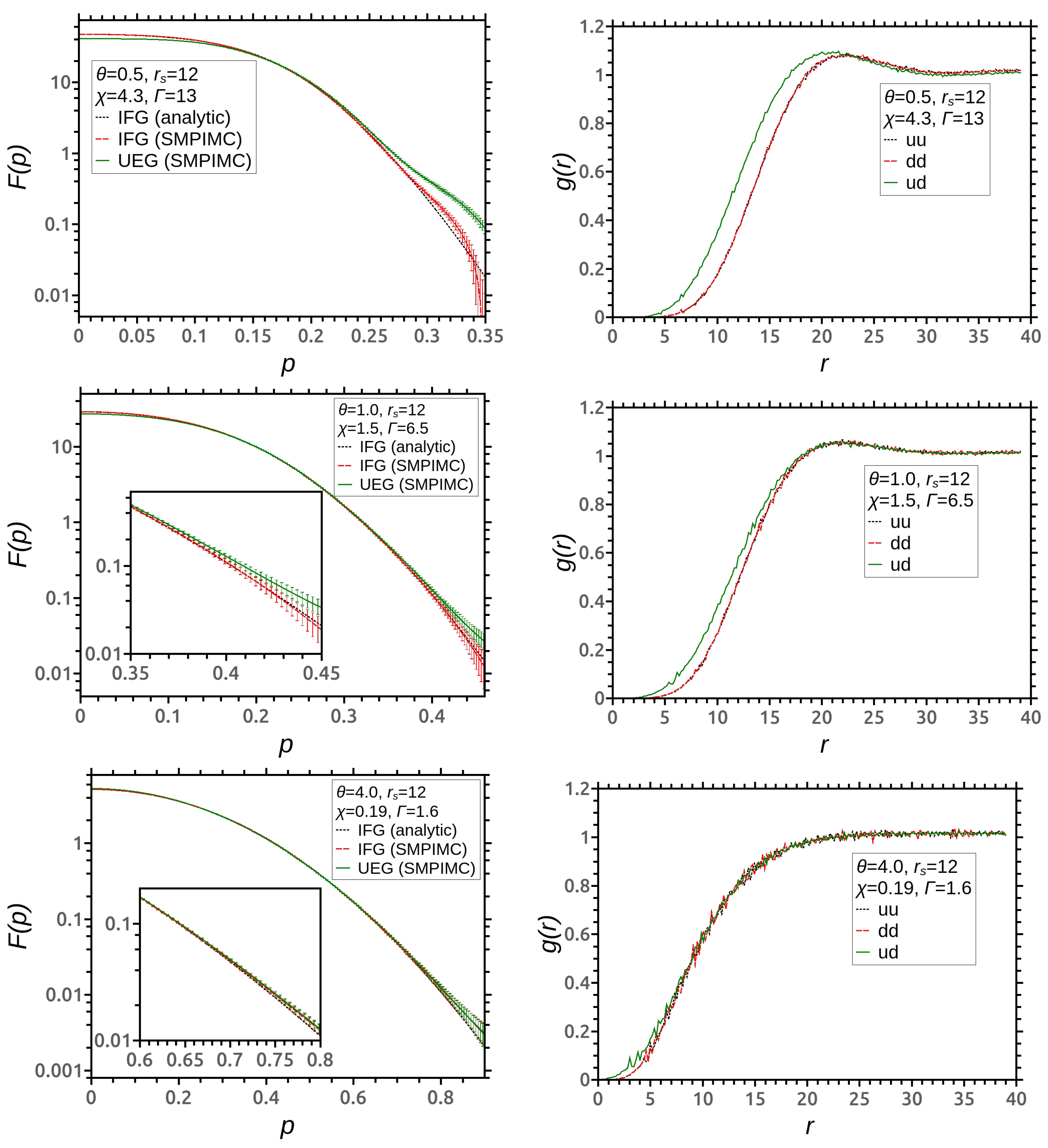
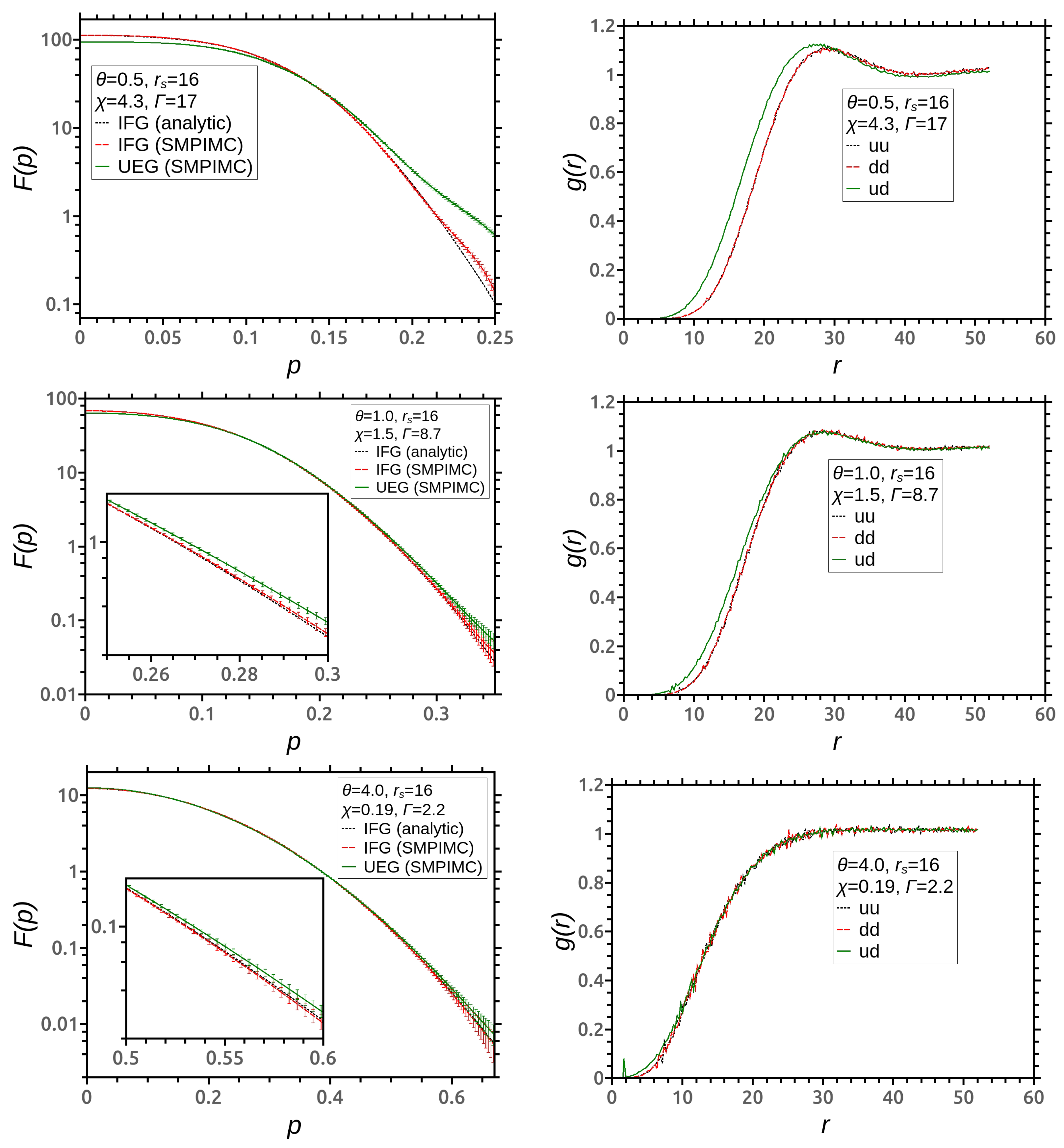
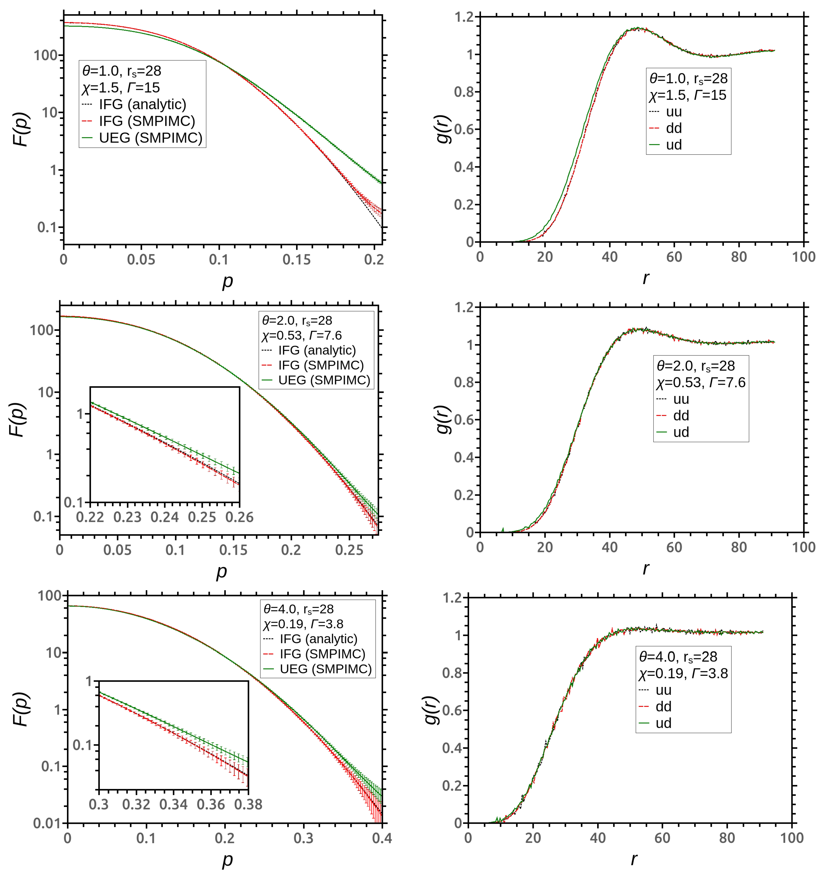
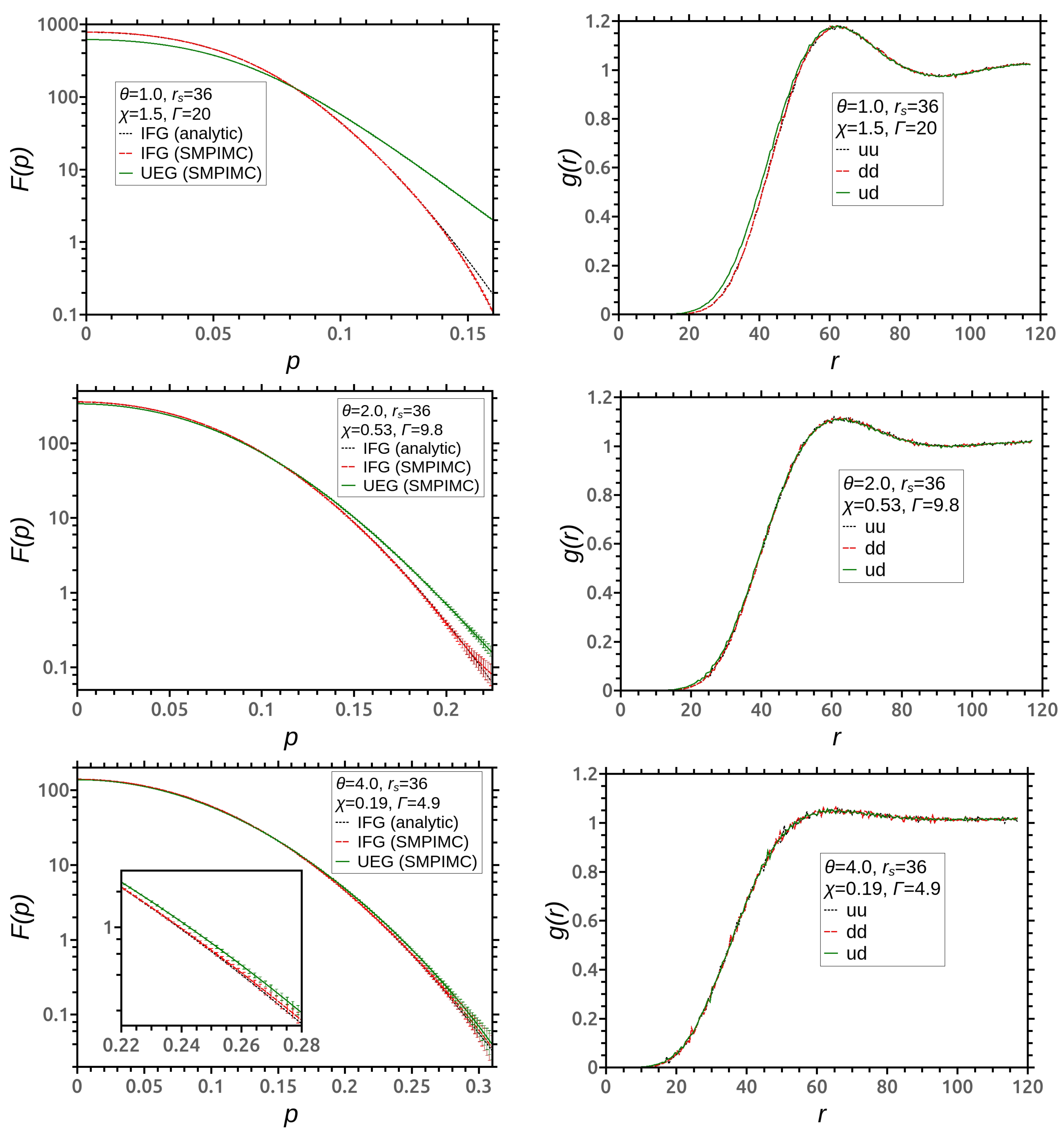
3. Simulation Results

We studied the unpolarized UEG in the range of densities and temperatures 0.2 r s 36 , 0.5 θ 4 , that corresponds to the coupling parameter 0.03 Γ 20 and the degeneracy parameter 0.2 χ 4 . Therefore, a wide range of states has been covered: from almost ideal to strongly non-ideal and, simultaneously, from an almost classical to degenerate system.
We carried out our simulations for N = 66 electrons in the cubic cell with PBCs. Such number of electrons has been chosen for conformity with the papers [34,36,41] and is quite enough for θ 0.5 . Furthermore, we simulated the unpolarized ideal Fermi gas (IFG) under the same conditions, i.e., the UEG with “turned-off” Coulomb interactions at the same θ and r s . Comparison of these results with the analytical Fermi distributions allows us to take into account the finite-size effects and control the related systematic errors in the MDF normalization factors. The influence of the finite-size effects on the MDFs manifests itself in the deviation of the calculated MDF for the IFG from the analytical Fermi distribution, which appears at some high value of momentum p F S , so the interval p p F S contains the reliable data. We estimated roughly the value of p F S from the plot of F ( p ) in the logarithmic scale. One can find the values of p F S for each plot in Table 1. This table also contains the approximate positions r m a x and r m i n of the first maximum and minimum of the PCFs g u u , g d d , and g u d .
For low values of r s ( r s 1 ), the UEG is characterized by relatively weak non-ideality ( Γ 1 in the considered range of θ ), and the results are quite trivial and do not deserve to be shown in figures. The MDFs completely coincide with the related Fermi distribution for p p F S . The PCFs are also similar to the ideal case: g u u and g d d , and are determined mainly by the exchange repulsion and slowly rise from 0 to 1 with growing r, while g u d is determined only by relatively weak Coulomb repulsion and rises much faster.
The results for r s = 4.0 are shown in Figure 1. In cases of θ = 0.5 and θ = 1 , the UEG is significantly non-ideal ( Γ 4.3 and Γ 2.2 ), while at θ = 4 it remains weakly coupled ( Γ 0.54 ). Although the difference between the MDFs and the related Fermi distribution does not exceed the statistical error in all cases, the PCFs demonstrate completely non-ideal behavior: g u d rises only slightly faster than g u u and g d d (especially at θ = 4.0 ) because of the same order of the Coulomb and exchange interactions.
The results for r s = 12.0 are shown in Figure 2. In the case of θ = 0.5 , the coupling is very strong ( Γ 13 ), and the MDF significantly differs from the Fermi distribution demonstrating an extensive “tail” at high momenta, which is not camouflaged by the finite-size effects. All PCFs have maxima exceeding 1 at r m a x , and g u d grows almost with the same rate as g u u and g d d , because the Coulomb repulsion plays a major role. In the case of θ = 1.0 , the coupling is quite strong ( Γ 6.5 ). The difference between MDF and the Fermi distribution does not exceed the statistical error. However, there are weak maxima on the PCFs, and g u d almost coincides with g u u and g d d . At θ = 4.0 , the UEG is significantly non-ideal ( Γ 1.6 ), the MDF does not differ from the Fermi distribution, and all the PCFs are the same and do not have any maxima.
The results for r s = 16.0 are shown in Figure 3. In the case of θ = 0.5 ( Γ 17 ), the MDF is quite similar to the previously considered one with r s = 12 , but the difference between it and the Fermi distribution is more significant. The PCFs are also analogous to the case of r s = 12 , but the maxima are more pronounced and the minima (at r m i n ) begin to appear. In the case of θ = 1.0 , the coupling is also strong ( Γ 8.7 ), and the MDF begins to differ from the Fermi distribution. The PCFs have distinct maxima at r 28 a 0 . In the case of θ = 4.0 , the coupling strength Γ 2.2 , and the MDF coincides with the Fermi distribution within the statistical error. The PCFs do not have any maxima yet, and there are no differences between g u u , g d d , and g u d , so the exchange interaction is negligible in comparison with the Coulomb one.
The results for r s = 28.0 are shown in Figure 4. In the case of θ = 1 , the UEG is strongly non-ideal ( Γ 15 ), and the MDF differs from the Fermi distribution very distinctly. All PCFs are almost the same and have maxima and minima. In the case of θ 2 , the coupling strength Γ 7.6 and non-ideality is quite strong. The MDF begins to deviate from the Fermi distribution, while the PCFs g u u , g d d , and g u d are exactly the same and have distinct maxima. In the case of θ 4.0 , the coupling strength Γ 3.8 , and the MDF, slightly differ from the Fermi distribution. The maxima of the PCFs are small but distinguishable.
The results for r s = 36.0 are shown in Figure 5. In the case of θ = 0.5 , the coupling strength is very strong ( Γ 20 ). The difference between the MDF and the Fermi distribution becomes more significant. The first maxima and minima of the PCFs become more pronounced, also, the second maxima starts to appear at r 120 a 0 ; however, the number of electrons should be increased for better resolution. In the case of θ 2 ( Γ 9.8 ), the MDF has quite a distinct “tail”. The PCFs g u u , g d d , and g u d are completely the same and have maxima and hardly distinguishable minima. In the case of θ 4.0 , the coupling strength Γ 4.9 , the MDF slightly differs from the Fermi distribution and there are maxima on the PCFs.
In addition, we calculated the average kinetic energy E k i n and potential energy E p o t of the UEG, supplementing our results from [34] with the strongly coupled states of UEG. These results are presented in Table 2 and Figure 6 and compared with the internal (kinetic) energy of the IFG, calculated with the SMPIMC method ( E I F G ) and obtained from the analytical Fermi distribution directly ( E I F G 0 ). The kinetic energy rapidly decreases by many orders of magnitude as the parameter r s increases, similar to the ideal case (for the Boltzmann gas E k i n r s 2 ). E k i n starts to exceed E I F G at high values of r s due to the effect of “quantum tails”; for example, E k i n becomes almost 30 % higher than E I F G at r s = 36 , θ = 0.5 . The potential energy is negative and rapidly falls as r s grows, while the dependence of E p o t on θ at fixed r s is more sharp at low values of r s and becomes weaker at high values (for the Boltzmann gas E p o t r s 1 ).

4. Discussion

First of all, let us discuss the phenomenon of “quantum tails” of the MDFs and make some suggestions about its physical nature. As it follows from Figure 1, Figure 2, Figure 3, Figure 4 and Figure 5, the single-particle MDF of the UEG starts to differ from the Fermi distribution when the system becomes strongly non-ideal. The value of the coupling parameter Γ , at which the “tail” appears, depends on the degeneracy rate: in the case of θ = 0.5 , (significant degeneracy) it appears at Γ from 8 to 9 ( r s 8 ), but in the case of θ = 4.0 , the Γ 5 is quite enough ( r s 36 ).
At the same time, the deviation of the MDFs from the Fermi distribution is always followed by the appearance of the visible maxima on the PCFs, and with increasing maxima, the deviation also grows. This observation points at a possible physical reason of “quantum tails”: with increasing non-ideality, the UEG becomes more liquid-like and the short-range order appears. This results in the potential wells surrounding the electrons at the average distance r m a x , so the spatial localization of the electrons increases. According to the basic principles of quantum mechanics, the localization of the electrons in the momentum space is weakened and the MDFs become wider. When the coupling increases, the potential wells become deeper and the effect grows.
Furthermore, this hypothesis can explain the fact that the “quantum tail” of the MDF appears at lower values of Γ when the degeneracy is low and at higher values in the opposite case. In fact, at low θ , the thermal wavelength λ becomes of the order of the interparticle distance, so the electron can escape from the potential well more easily via the quantum tunneling and becomes less localized. Note that the definition of the coupling strength Γ is based on the classical value of the average kinetic energy k T and gives an overestimated value of the actual non-ideality in the degenerate case, which should be characterized by the quantum average kinetic energy between k T and E F . Thus, at the same values of Γ , a non-degenerate system (high θ ) is more non-ideal than a degenerate one (low θ ), and the ”quantum tail” effect is more significant.
Secondly, the difference between PCFs g u u , g d d , and g u d becomes lower with increasing r s even at low values of θ (degenerate case). As the exchange repulsion is applied only to the electrons with the same spin projections, while the Coulomb interaction is universal, we can conclude that the PCFs of the degenerate UEG are basically conditioned by the last one. This reasoning is confirmed by the fact that the value of r m a x is almost independent of θ when r s is fixed. However, the value of the maxima depends strongly on θ , following the coupling strength Γ .

5. Conclusions

In this paper, we have continued our research of the UEG and study the MDFs and the PCFs using the SMPIMC method in a wide range of temperatures and densities: 0.5 θ 4 , 0.2 r s 36 . Thus, different thermodynamic states from an almost ideal gas (Boltzmann of Fermi) to a strongly non-ideal system with weak and significant degeneracy have been considered.
Firstly, we have discovered that the single-particle MDFs start to exceed the Fermi distribution at high momentum values, when the UEG is strongly non-ideal. In the degenerate case θ = 0.5 , this occurs at r s 8 ( Γ 9 ), in the semi-degenerate case θ = 1 —at r s 16 ( Γ 8 ), in the almost classical case θ = 4 —at r s = 36 ( Γ 5 ). The deviation has the form of the “quantum tail” at high momenta and is reliable at p p F S , where the value of p F S is conditioned by the finite-size effects.
We explain the phenomena of “quantum tails” as follows. The deviation of the MDFs from the Fermi distribution is always followed by the appearance of the short-range order on the PCFs; so, with increasing coupling strength, the UEG becomes more liquid-like and the potential wells surrounding the electrons appear. As a result, the spatial localization of the electrons increases, so the localization in the momentum space becomes weaker and the MDFs become wider. Besides, at high degeneracy, the electrons are tunneling from the potential wells more easily, so the “quantum tail” appears at higher values of Γ in comparison with the non-degenerate case.
Secondly, we have obtained that the difference between the PCFs of the electrons with the same and opposite spin projections becomes negligible at high values of Γ in the degenerate case. Thus, the spatial structure of a strongly non-ideal UEG is basically conditioned by the Coulomb interaction rather than the exchange repulsion.
Finally, we have calculated the average kinetic and potential energies for r s up to 36, supplementing our results from [34] significantly.

Author Contributions

Conceptualization, A.L. and V.F.; methodology, A.L.; software, A.L.; validation, A.L., V.F. and P.L.; investigation, A.L.; visualization, A.L.; writing—original draft preparation, A.L.; writing—review and editing, V.F. and P.L.; supervision, V.F.; project administration, P.L.; funding acquisition, V.F. and P.L. All authors have read and agreed to the published version of the manuscript.

Funding

This research was supported by the by the Russian Science Foundation, Grant No. 20-42-04421.

Institutional Review Board Statement

Not applicable.

Informed Consent Statement

Not applicable.

Data Availability Statement

The data that support the findings of this study are available from the corresponding author upon reasonable request.

Acknowledgments

We acknowledge stimulating discussions with M. Bonitz, T. Schoof, S. Groth, and T. Dornheim (Kiel).

Conflicts of Interest

The authors declare no conflict of interest.

Abbreviations

The following abbreviations are used in this manuscript:
CPIMCConfiguration Path Integral Monte Carlo
DFTDensity Functional Theory
IFGIdeal Fermi Gas
MDFMomentum Distribution Function
PBCPeriodic Boundary Conditions
PCFPair Correlation Function
SMPIMCSingle Momentum Path Integral Monte Carlo
UEGUniform Electron Gas
WDMWarm Dense Matter

Appendix A. Numerical Method SMPIMC

Appendix A.1. Basic Idea of Path Integral Monte Carlo Methods

Let us consider a multiple integral defining the average value of a function a ( x ) with a distribution function f ( x ) (sign-alternating in general case):
a f = 1 Z a ( x ) f ( x ) d n x , Z = f ( x ) d n x ,
where Z is the normalization factor. Replacing the sign-alternating distribution function with the product of the normalized absolute value w ( x ) = | f ( x ) | / C and the weight function g ( x ) = sign f ( x ) , one can give the probabilistic interpretation of (A1):
a f = a g w g w , where b w = b ( x ) w ( x ) d n x .
Now, the function w ( x ) , can be interpreted as the probability density for a random vector x . The basic idea of a Monte Carlo method is to estimate the integral via averaging the integrands over a random sample with the probability density w ( x ) :
a f i = 1 N a ( x i ) g ( x i ) i = 1 N m c g ( x i ) .
If random vectors x i in the sample are not correlated, the statistical error is O ( N 1 / 2 ) , and can be estimated via 3 σ -rule according to the law of large numbers.
The sample { x 1 , x 2 , , x N m c } can be created via the Metropolis algorithm [42]. This algorithm consists of sequential steps divided into two sub-steps: the proposal and the acceptance. If the value of a random vector on the i-th step is x i , and a new random value x i uniformly distributed in some n-dimensional cube is proposed, this new state has to be accepted with the probability:
A ( x i x i ) = max 1 , w ( x i + 1 ) w ( x i ) .
In the case of acceptance, the state on the i + 1 step becomes x i + 1 = x i , and in the case of rejection, the old value is saved: x i + 1 = x i . Performing N m c steps of the Metropolis algorithm gives us the required sample.

Appendix A.2. Periodic Boundary Conditions

Available computer resources do not allow us to simulate macroscopic systems, so the number of electrons in the simulation box is limited. Since the concentration N / V is constant, the volume V is relatively small and the finite-size effects can be significant. To reduce them and reproduce the properties of a macroscopic system as accurately as possible, we consider a cubic main cell with side length L = V 1 / 3 and periodic boundary conditions (PBC) [43]. When any bead q a , k leaves the simulation box, it should be replaced with the periodic image, entering into the main cell instead:
q a , i k q a , i k L q a , i k L + 1 2 ( i = x , y , z ) .
Here, [ x ] means the floor integer value of x. In calculations of the distances between two beads Δ q a b , k , the nearest images should be taken:
Δ q a b , k , i Δ q a b , k , i L Δ q a b , k , i L + 1 2 ( i = x , y , z ) .
In calculations of the ξ -distribution, one has also to “periodize” the coordinates ξ a before adding them to the histogram:
ξ a , i ξ a , i L ξ a , i L + 1 2 ( i = x , y , z ) .

Appendix A.3. Smpimc Algorithm for PCFs

Calculation of PCFs with the SMPIMC method is based on the definition (5) and representation (26) of the diagonal density matrix ρ D G . Integration over the variables q a and z a k is performed using the Monte Carlo approach. Electron a in the simulation box is represented as the closed poly-line with vertices q a k = q a + z a k , so that the “center”-coordinate q a describes the position of the whole a-th electron, and the “bead”-coordinate z a k —the relative position of the k-th bead. Note that only coordinates q a are used in the calculations of PCFs directly, while the beads are “inner” coordinates and define the weight and probability density of the configuration. The detailed SMPIMC algorithm for the calculation of PCFs is presented below.
  • Set the run number l = 0 and the initial state x 0 : the coordinates q a are uniformly distributed in the simulation box, the coordinates z a k are equal to zero ( a = 1 , , N , k = 0 , , M ).
  • Set the step number i = 1 and the first state x 1 = x 0 .
  • Select the particle number a = 1 , , N randomly, then select the type of the step: δ q –step with the probability P q or δ z –step with the probability P z = 1 P q . If δ q –step has been chosen, modify q a q a + Δ q with Δ q uniformly distributed in the volume L 3 / N . If δ z –step has been chosen, select the bead number k = 1 , , M 1 randomly and modify z a k z a k + Δ z with Δ z uniformly distributed in the volume λ 3 / ( 4 π K ) 3 / 2 . In both cases, take into account the PBC. The resulting state has to be set as the proposed state x i .
  • Accept the proposed state x i with the probability A ( x i x i ) (A4) or reject it. In the case of acceptance—set x i + 1 = x i , in the case of rejection—set x i + 1 = x i .
  • Calculate the distances between each pair of electrons r a b = | q a q b | and build the related histograms: h u u n ( x i ) , h d d n ( x i ) and h u d n ( x i ) , where n = 1 , , N q is the cell number with the length Δ r , so n = r a b / Δ r + 1 .
  • Repeat steps (3)–(5) for i = 1 , , N s t e p s .
  • Calculate the average histograms for the obtained sample of N s t e p s states via averaging of h u u n , h d d n and h u d n with g ( x ) as the weight function:
    h s 1 s 2 n l = i = 1 N s t e p s h s 1 s 2 n ( x i ) g ( x i ) i = 1 N s t e p s g ( x i ) ( s 1 , s 2 = { u , d } ) .
  • Repeat steps (2)–(7) for l = 1 , 2 , , N r u n s , but instead of initialization x 1 = x 0 use the last state from the previous run: x 1 | l = x N s t e p s | l 1 .
  • As a result, the sample of average histograms h s 1 s 2 n l , l = 0 , 1 , , N r u n s is obtained. Considering the 0-th run as idle and omitting it to eliminate the influence of the initial state, calculate the resulting average histograms over the sample and the statistical errors as follows:
    h s 1 s 2 n = l = 1 N r u n s h s 1 s 2 n l N r u n s , σ ( h s 1 s 2 n ) = l = 1 N r u n s ( h s 1 s 2 n l h s 1 s 2 n ) N r u n s .
  • To obtain the final histograms of the PCFs with the statistical errors one takes into account the angular distribution and the numbers of electron pairs for different spin projections:
    g s 1 s 2 n = h s 1 s 2 n Δ n C s 1 s 2 , σ ( g s 1 s 2 n ) = σ ( h s 1 s 2 n ) Δ n C s 1 s 2 ,
    where Δ n = 4 π Δ r 3 n 2 n + 1 / 3 , C s 1 s 2 is equal to N u ( N u 1 ) / 2 , N d ( N d 1 ) / 2 and N u N d for s 1 , s 2 equal to u,u; d,d and u,d, respectively.

Appendix A.4. Smpimc Algorithm for MDFs

Calculation of the single-particle MDF is based on the sine transform (14) of the ξ -distribution, which is obtained from the path integral representation (26) via the Monte-Carlo procedure similar to the one for PCFs. The difference is that the first electron is represented as the open poly-line with the vertices q 1 k = z 1 k + 1 k / M q 1 + ξ / 2 + k / M q 1 ξ / 2 . Only the differential coordinate ξ participates in the calculation of the single-particle MDF, while the other coordinates define only the weight and probability density. The detailed SMPIMC algorithm for the calculation of the single-particle MDF is presented below.
  • Set the run number l = 0 and the initial state x 0 : the coordinates q a are uniformly distributed in the simulation box, while the relative coordinates z a k and the differential coordinate ξ are equal to zero.
  • Set the step number i = 1 and the first state x 1 = x 0 .
  • Select the type of step: δ ξ –step with the probability P ξ , δ q –step with the probability P q or δ z –step with the probability P z = 1 P ξ P q . If δ ξ –step has been chosen, modify ξ ξ + Δ ξ with Δ ξ uniformly distributed in the volume λ 3 . Otherwise, select the particle number a = 1 , , N randomly; if δ q –step has been chosen, modify q a q a + Δ q with Δ q uniformly distributed in the volume L 3 / N ; if δ z –step has been chosen, select the “bead” number k = 1 , , M 1 randomly and modify z a k z a k + Δ z with Δ z uniformly distributed in the volume λ 3 / ( 4 π K ) 3 / 2 . Take into account the PBC. The resulting state has to be set as the proposed state x i .
  • Accept the proposed state x i with the probability A ( x i x i ) (A4) or reject it. In the case of acceptance, set x i + 1 = x i , in the case of rejection, set x i + 1 = x i .
  • Calculate the absolute value ξ = | ξ | and build the related histogram F Ω n ( x i ) , where n = 1 , , N ξ is the number of the cell with the length Δ ξ , so n = ξ / Δ ξ + 1 .
  • Repeat steps (3)–(5) for i = 1 , , N s t e p s .
  • Calculate the average histogram for the obtained sample of N s t e p s states via the averaging of f Ω n with g ( x ) as the weight function:
    f Ω n l = i = 1 N s t e p s f Ω n ( x i ) g ( x i ) i = 1 N s t e p s g ( x i ) .
  • To obtain the histogram of the ξ -distribution on the l-th run take into account the angular distribution:
    f n l = f Ω n l Δ n , Δ n = 4 π Δ ξ 3 n 2 n + 1 / 3 .
  • Repeat steps (2)–(8) for l = 1 , 2 , , N r u n s , but instead of the initialization x 1 = x 0 use the last state from the previous run: x 1 | l = x N s t e p s | l 1 .
  • As a result, the sample of average histograms of ξ -distribution f n l , l = 0 , 1 , , N r u n s is obtained. Considering the 0-th run as idle and omitting it to eliminate the influence of the initial state, calculate the resulting average histogram over the sample with the statistical error as follows:
    f n = l = 1 N r u n s f n l N r u n s , σ ( f n ) = l = 1 N r u n s ( f n l f n ) N r u n s .
  • To obtain the histogram of the MDF perform the discrete sine transform of the lattice function f ( ξ n ) = f n :
    F ( p ) = n = 1 N ξ Δ ξ 4 π ξ n 2 f ( ξ n ) sin p ξ n / p ξ n / ,
    for the lattice values of p. The statistical error can be easily calculated via a similar procedure.

References

  1. Knudson, M.D.; Desjarlais, M.P.; Lemke, R.W.; Mattsson, T.R.; French, M.; Nettelmann, N.; Redmer, R. Probing the Interiors of the Ice Giants: Shock Compression of Water to 700 GPa and 3.8 g/cm3. Phys. Rev. Lett. 2012, 108, 091102. [Google Scholar] [CrossRef] [PubMed]
  2. Nettelmann, N.; Becker, A.; Holst, B.; Redmer, R. Jupiter models with Improved ab initio hydrogen equation of state (H-REOS.2). Astrophys. J. 2012, 750, 52. [Google Scholar] [CrossRef] [Green Version]
  3. Mazevet, S.; Licari, A.; Chabrier, G.; Potekhin, A.Y. Ab initio based equation of state of dense water for planetary and exoplanetary modeling. Astron. Astrophys. 2019, 621, A128. [Google Scholar] [CrossRef] [Green Version]
  4. Hubbard, W.B.; Guillot, T.; Lunine, J.I.; Burrows, A.; Saumon, D.; Marley, M.S.; Freedman, R.S. Liquid metallic hydrogen and the structure of brown dwarfs and giant planets. Phys. Plasmas 1997, 4, 2011–2015. [Google Scholar] [CrossRef] [Green Version]
  5. Chabrier, G.; Brassard, P.; Fontaine, G.; Saumon, D. Cooling Sequences and Color-Magnitude Diagrams for Cool White Dwarfs with Hydrogen Atmospheres. Astrophys. J. 2000, 543, 216–226. [Google Scholar] [CrossRef]
  6. Haensel, P.; Potekhin, A.Y.; Yakovlev, D.G. Neutron Stars 1: Equation of State and Structure; Astrophysics and Space Science Library; Springer: New York, NY, USA, 2007. [Google Scholar] [CrossRef]
  7. Sharma, B.K.; Centelles, M.; Viñas, X.; Baldo, M.; Burgio, G.F. Unified equation of state for neutron stars on a microscopic basis. Astron. Astrophys. 2015, 584, A103. [Google Scholar] [CrossRef]
  8. Schmit, P.F.; Knapp, P.F.; Hansen, S.B.; Gomez, M.R.; Hahn, K.D.; Sinars, D.B.; Peterson, K.J.; Slutz, S.A.; Sefkow, A.B.; Awe, T.J.; et al. Understanding Fuel Magnetization and Mix Using Secondary Nuclear Reactions in Magneto-Inertial Fusion. Phys. Rev. Lett. 2014, 113, 155004. [Google Scholar] [CrossRef] [Green Version]
  9. Nora, R.; Theobald, W.; Betti, R.; Marshall, F.J.; Michel, D.T.; Seka, W.; Yaakobi, B.; Lafon, M.; Stoeckl, C.; Delettrez, J.; et al. Gigabar Spherical Shock Generation on the OMEGA Laser. Phys. Rev. Lett. 2015, 114, 045001. [Google Scholar] [CrossRef]
  10. Roozehdar Mogaddam, R.; Sepehri Javan, N.; Javidan, K.; Mohammadzadeh, H. Modulation instability and soliton formation in the interaction of X-ray laser beam with relativistic quantum plasma. Phys. Plasmas 2019, 26, 062112. [Google Scholar] [CrossRef]
  11. Edwards, M.R.; Shi, Y.; Mikhailova, J.M.; Fisch, N.J. Laser amplification in strongly magnetized plasma. Phys. Rev. Lett. 2019, 123, 025001. [Google Scholar] [CrossRef] [Green Version]
  12. Ebeling, W.; Fortov, V.; Filinov, V. Quantum Statistics of Dense Gases and Nonideal Plasmas; Springer: Berlin, Germany, 2017. [Google Scholar]
  13. Savchenko, V.I. Quantum, multibody effects and nuclear reaction rates in plasmas. Phys. Plasmas 2001, 8, 82–91. [Google Scholar] [CrossRef] [Green Version]
  14. Salpeter, E.E.; van Horn, H.M. Nuclear Reaction Rates at High Densities. Astrophys. J. 1969, 155, 183. [Google Scholar] [CrossRef]
  15. Ichimaru, S. Nuclear fusion in dense plasmas. Rev. Mod. Phys. 1993, 65, 255–299. [Google Scholar] [CrossRef]
  16. Dewitt, H.; Slattery, W. Screening Enhancement of Thermonuclear Reactions in High Density Stars. Contrib. Plasma Phys. 1999, 39, 97–100. [Google Scholar] [CrossRef] [Green Version]
  17. Starostin, A.; Mironov, A.; Aleksandrov, N.; Fisch, N.; Kulsrud, R. Quantum corrections to the distribution function of particles over momentum in dense media. Physica A 2002, 305, 287–296. [Google Scholar] [CrossRef]
  18. Starostin, A.; Leonov, A.; Petrushevich, Y. Quantum corrections to the particle distribution function and reaction rates in dense media. Plasma Phys. Rep. 2005, 31, 123–132. [Google Scholar] [CrossRef]
  19. Starostin, A.; Gryaznov, V.; Petrushevich, Y. Development of the theory of momentum distribution of particles with regard to quantum phenomena. J. Exp. Theor. Phys. 2017, 125, 940–947. [Google Scholar] [CrossRef]
  20. Larkin, A.S.; Filinov, V.S.; Fortov, V.E. Path Integral Representation of the Wigner Function in Canonical Ensemble. Contrib. Plasma Phys. 2016, 56, 187–196. [Google Scholar] [CrossRef]
  21. Larkin, A.; Filinov, V. Phase Space Path Integral Representation for Wigner Function. J. Appl. Math. Phys. 2017, 5, 392–411. [Google Scholar] [CrossRef] [Green Version]
  22. Larkin, A.; Filinov, V. Quantum tails in the momentum distribution functions of non-ideal Fermi systems. Contrib. Plasma Phys. 2018, 58, 107–113. [Google Scholar] [CrossRef]
  23. Larkin, A.; Filinov, V.; Fortov, V. Peculiarities of the momentum distribution functions of strongly correlated charged fermions. J. Phys. A Math. Theor. 2017, 51, 035002. [Google Scholar] [CrossRef] [Green Version]
  24. Larkin, A.; Filinov, V.; Fortov, V. Pauli blocking by effective pair pseudopotential in degenerate Fermi systems of particles. Contrib. Plasma Phys. 2017, 57, 506–511. [Google Scholar] [CrossRef]
  25. Larkin, A.S.; Filinov, V.S. Monte Carlo simulation of the thermodynamic properties of hydrogen plasma with the Wigner function. High Temp. 2019, 57, 651–659. [Google Scholar] [CrossRef]
  26. Jones, R.O. Density functional theory: Its origins, rise to prominence, and future. Rev. Mod. Phys. 2015, 87, 897–923. [Google Scholar] [CrossRef] [Green Version]
  27. Karasiev, V.V.; Sjostrom, T.; Dufty, J.; Trickey, S.B. Accurate Homogeneous Electron Gas Exchange-Correlation Free Energy for Local Spin-Density Calculations. Phys. Rev. Lett. 2014, 112, 076403. [Google Scholar] [CrossRef]
  28. Chachiyo, T. Communication: Simple and accurate uniform electron gas correlation energy for the full range of densities. J. Chem. Phys. 2016, 145, 021101. [Google Scholar] [CrossRef]
  29. Loos, P.F.; Gill, P.M.W. The uniform electron gas. WIREs Comput. Mol. Sci. 2016, 6, 410–429. [Google Scholar] [CrossRef]
  30. Mahan, G. Many-Particle Physics; Physics of Solids and Liquids; Springer: New York, NY, USA, 2000. [Google Scholar]
  31. Yasuhara, H.; Kawazoe, Y. A note on the momentum distribution function for an electron gas. Phys. A 1976, 85, 416–424. [Google Scholar] [CrossRef]
  32. Kimball, J.C. Short-range correlations and the structure factor and momentum distribution of electrons. J. Phys. A Math. Gen. 1975, 8, 1513–1517. [Google Scholar] [CrossRef]
  33. Hunger, K.; Schoof, T.; Dornheim, T.; Bonitz, M.; Filinov, A. Momentum distribution function and short-range correlations of the warm dense electron gas: Ab initio quantum Monte Carlo results. Phys. Rev. E 2021, 103, 053204. [Google Scholar] [CrossRef]
  34. Larkin, A.S.; Filinov, V.S.; Levashov, P.R. Single-momentum path integral Monte Carlo simulations of uniform electron gas in warm dense matter regime. Phys. Plasmas 2021, 28, 122712. [Google Scholar] [CrossRef]
  35. Toukmaji, A.Y.; Board, J.A. Ewald summation techniques in perspective: A survey. Comput. Phys. Commun. 1996, 95, 73–92. [Google Scholar] [CrossRef]
  36. Dornheim, T.; Groth, S.; Bonitz, M. The uniform electron gas at warm dense matter conditions. Phys. Rep. 2018, 744, 1–86. [Google Scholar] [CrossRef] [Green Version]
  37. Tatarskiĭ, V.I. The Wigner representation of quantum mechanics. PHYS-USP+ 1983, 26, 311–327. [Google Scholar] [CrossRef]
  38. Feynman, R.; Hibbs, A. Quantum Mechanics and Path-Integral; Physics of Solids and Liquids; McGraw-Hill: New York, NY, USA, 1965. [Google Scholar]
  39. Filinov, V.S.; Bonitz, M.; Levashov, P.; Fortov, V.E.; Ebeling, W.; Schlanges, M.; Koch, S.W. Plasma phase transition in dense hydrogen and electron–hole plasmas. J. Phys. A Math. Gen. 2003, 36, 6069–6076. [Google Scholar] [CrossRef] [Green Version]
  40. Kleinert, H. Path Integrals in Quantum Mechanics, Statistics, Polymer Physics, and Financial Markets; World Scientific: Singapore, 2004. [Google Scholar]
  41. Dornheim, T.; Groth, S.; Schoof, T.; Hann, C.; Bonitz, M. Ab initio quantum Monte Carlo simulations of the uniform electron gas without fixed nodes: The unpolarized case. Phys. Rev. B 2016, 93, 205134. [Google Scholar] [CrossRef] [Green Version]
  42. Hastings, W.K. Monte Carlo sampling methods using Markov chains and their applications. Biometrika 1970, 57, 97–109. [Google Scholar] [CrossRef]
  43. Allen, M.; Tildesley, D. Computer Simulation of Liquids; Clarendon Press: Oxford, UK, 1988. [Google Scholar]
Figure 1. Left plots: single-particle momentum distribution functions of the unpolarized UEG at r s = 4.0 and θ = 0.5 , 1 , 4 calculated with the SMPIMC method. The results are compared with the SMPIMC results for the IFG in the same conditions and with the analytical Fermi distributions. Right plots: the pair correlation functions g u u , g d d , and g u d of the UEG.
Mathematics 10 02270 g001
Figure 2. Left plots: single-particle MDFs of the unpolarized UEG at r s = 12 and θ = 0.5 , 1 , 4 calculated with the SMPIMC method. The results are compared with the SMPIMC for the IFD at the same conditions and with the analytical Fermi distributions. Right plots: PCFs g u u , g d d and g u d of the UEG.
Mathematics 10 02270 g002
Figure 3. Left plots: single-particle MDFs of the unpolarized UEG at r s = 16 and θ = 0.5 , 1 , 4 calculated with the SMPIMC method. The results are compared with the SMPIMC for the IFG at the same conditions, and with the analytical Fermi distributions. Right plots: PCFs g u u , g d d , and g u d of the UEG.
Mathematics 10 02270 g003
Figure 4. Left plots: single-particle MDFs of the unpolarized UEG at r s = 28 and θ = 0.5 , 1 , 4 calculated with the SMPIMC method. The results are compared with the SMPIMC for the IFG at the same conditions and with the analytical Fermi distributions. Right plots: PCFs g u u , g d d , and g u d of the UEG.
Mathematics 10 02270 g004
Figure 5. Left plots: single-particle MDFs of the unpolarized UEG at r s = 36 and θ = 0.5 , 1 , 4 calculated with the SMPIMC method. The results are compared with the SMPIMC for the IFG at the same conditions and with the analytical Fermi distributions. Right plots: PCFs g u u , g d d , and g u d of the UEG.
Mathematics 10 02270 g005
Figure 6. Left plot: average kinetic energy of the UEG at different values of r s and θ compared with the internal (kinetic) energy of the IFG. Right plot: average potential energy of the UEG.
Mathematics 10 02270 g006
Table 1. Some parameters and data describing the MDFs and PCFs from the Figure 1, Figure 2, Figure 3, Figure 4 and Figure 5. The values are shown with two significant digits.
r s θ Γ χ λ , a 0 L , a 0 p F S , / a 0 r m a x , a 0 r m i n , a 0
4.0 0.5 4.3 4.3 1026 0.85
4.0 1.0 2.2 1.5 7.4 26 1.2
4.0 4.0 0.54 0.19 3.7 26>1.9
12 0.5 13 4.3 3178 0.28 20–2230–32
12 1.0 6.5 1.5 2278 0.42 20–22
12 4.0 1.6 0.19 1178 0.65
16 0.5 17 4.3 42100 0.21 26–2840–42
16 1.0 8.7 1.5 30100 0.30 26–28
16 4.0 2.2 0.19 15100 0.60
28 1.0 15 1.5 52180 0.17 45–5070
28 2.0 7.6 0.53 37180 0.26 45–5070–75
28 4.0 3.8 0.19 26180 0.38 50
36 1.0 20 1.5 66230 0.14 60–6590
36 2.0 9.8 0.53 47230 0.21 60–6590–95
36 4.0 4.9 0.19 33230 0.28 60–65
Table 2. E I F G 0 —internal (kinetic) energy of the macroscopic IFG obtained from the analytical Fermi distribution; E I F G —internal (kinetic) energy of the finite-size IFG obtained from the SMPIMC; E k i n and E p o t —kinetic and potential energy of the UEG. Two significant digits of the statistical error 3 σ are written in brackets. All energies are given per one electron.
r s θ E IFG 0 , Ha E IFG , Ha E kin , Ha E pot , Ha
4.0 0.5 0.118 0.118 ( 02 ) 0.121 ( 02 ) 0.22386 ( 12 )
4.0 1.0 0.195 0.197 ( 05 ) 0.195 ( 05 ) 0.21480 ( 10 )
4.0 4.0 0.702 0.702 ( 18 ) 0.699 ( 18 ) 0.17822 ( 14 )
12 0.5 0.0131 0.0131 ( 01 ) 0.0141 ( 03 ) 0.081073 ( 40 )
12 1.0 0.0217 0.0216 ( 03 ) 0.0224 ( 04 ) 0.079157 ( 35 )
12 4.0 0.0780 0.0793 ( 18 ) 0.0789 ( 18 ) 0.070567 ( 24 )
16 0.5 0.00735 0.00735 ( 05 ) 0.00841 ( 12 ) 0.061467 ( 25 )
16 1.0 0.0122 0.0123 ( 02 ) 0.0126 ( 02 ) 0.060535 ( 18 )
16 4.0 0.0439 0.0438 ( 10 ) 0.0446 ( 09 ) 0.054942 ( 17 )
28 1.0 0.00399 0.00402 ( 02 ) 0.00464 ( 03 ) 0.035732 ( 12 )
28 2.0 0.00738 0.00735 ( 08 ) 0.00755 ( 09 ) 0.034815 ( 10 )
28 4.0 0.0143 0.0143 ( 02 ) 0.0149 ( 02 ) 0.033396 ( 10 )
36 1.0 0.00241 0.00240 ( 00 ) 0.00314 ( 00 ) 0.028246 ( 08 )
36 2.0 0.00446 0.00446 ( 04 ) 0.00480 ( 04 ) 0.027628 ( 10 )
36 4.0 0.00867 0.00869 ( 11 ) 0.00894 ( 12 ) 0.026520 ( 05 )
Publisher’s Note: MDPI stays neutral with regard to jurisdictional claims in published maps and institutional affiliations.

